MODEL

Consider a simple two-party model of one electoral constituency in which the outcome in any given election is determined by a long-term “normal vote” and a short-term “shock.” Let μ _D denote the normal vote and let η denote the shock, where μ _D is a real number and η is a random variable. The vote-percentage for the Democratic candidate is V=μ _D +η. Suppose μ _D >50, so the constituency tends to favor Democratic candidates. Even though Democrats are favored, if η is negative and large enough in magnitude, then the Democrat might lose. Also, if η is near 50−μ _D , then the outcome will be near 50–50 (that is, the race will be “close”). Note that η incorporates all factors other than the normal vote that affect election outcomes, such as partisan tides, candidates’ relative qualities, incumbency advantages, national and local economic shocks, cross-cutting or wedge issues, and campaign strategies and tactics.

Suppose η has a normal distribution; that is, $$\eta \sim N(0,\sigma _{D}^{2} )$$ . Then $$V \sim N(\mu _{D} ,\sigma _{D}^{2} )$$ .Footnote ⁶ Suppose we are researchers with access to a large number of election outcomes for the constituency, and we attempt an RDD with a window of [50−δ, 50+δ], where δ is “small,” say 1, 2 or 3. Figure 1 presents an example, with μ _D =60 and δ=2. As the figure makes clear, we do not expect to see the Democratic candidate winning 50 percent of the time in this window. The shaded area to the right of the line at the 50 percent threshold shows where the Democratic candidate wins, and the shaded area to the left of the threshold shows where the Republican candidate wins. Since the area on the right is clearly larger than that on the left, we expect to see the Democrat win more than 50 percent of the time.

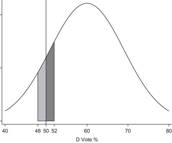
Fig. 1 Illustration of share of Democratic wins in close elections in Democratic-leaning districts. Note: distribution is normal with mean of 60 percent and standard deviation of 6 percent; window used to define close elections is 2 percent.

How much more? Consider a linear approximation of the density function of V around 50 percent. The density of V is $$f(V)=(2\pi \sigma _{D}^{2} )^{{{\minus}1/2}} exp({\minus}(v{\minus}\mu _{D} )^{2} /2\sigma _{D}^{2} )$$ . The slope of this density at V=50 is $$f^{'} (50)=(\mu _{D} {\minus}50)f(50)/\sigma _{D}^{2} $$ . The probability that the Democratic candidate will win given that V∈[50−δ, 50+δ] is then approximately

(1) $$P_{D} ={{\delta f\left( {50} \right){\plus}\delta ^{2} f^{'} \left( {50} \right)/2} \over {\left 2{\delta f\left( {50} \right)\right}}$$

(2) $$\qquad ={{\delta f\left( {{\rm 50}} \right)\left[ {2{\plus}\delta (\mu _{D} {\minus}50)/\sigma _{D}^{2} } \right]} \over {4\delta f\left( {50} \right)}}$$

(3) $$={1 \over 2}{\plus}{{\delta \left( {\mu _{D} {\minus}50} \right)} \over {4\sigma _{D}^{2} }}{\rm .} \ \qquad$$

For US House elections from 1980–2010, the average within-district standard deviation of the Democratic percentage of the two-party vote is about 6.3. So, to be conservative, we set σ _D=6. Suppose, for example, that the window is plus or minus 2 percentage points around the 50 percent threshold (δ=2). Thus in a district that is 60 percent Democratic (μ _D =60), the probability that the Democratic candidate will win is approximately 0.5+20/144=0.64. So in this case, we should expect to see Democrats winning about 64 percent of the races in a 2 percentage point window around the 50–50 threshold, not 50 percent of the races. Even in the small window of 49–51 percent, the Democrats are expected to win about 57 percent of the races.

Figure 2 shows exact calculations based on the normal density function, rather than linear approximations; it presents the calculations for σ _D =9 (which is slightly larger than the within-state standard deviation of the Democratic percentage of the two-party vote from 1980–2008). Evidently, many of the numbers are much larger than 50 percent, especially when δ≥2.Footnote ⁷

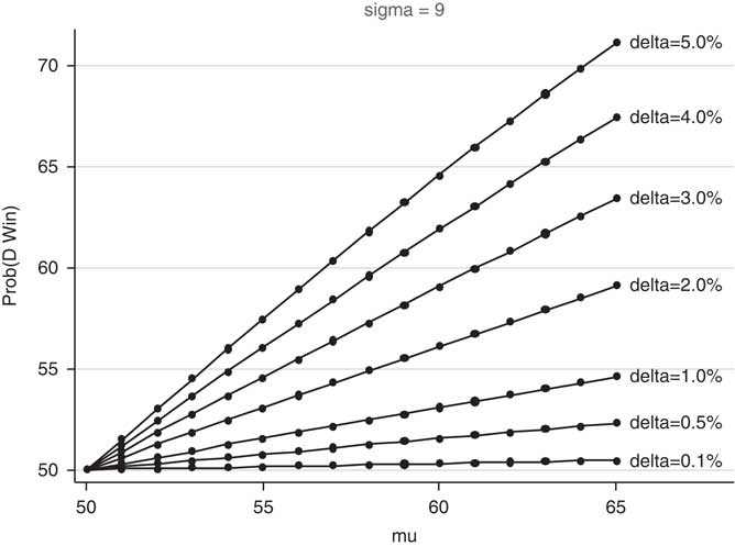
Fig. 2 Probability of a Democratic win in a close election as a function of Democratic normal vote (μ_D). Note: standard deviation (sigma) of 9 percent. The relationship is shown for seven definitions of close elections (δ).

IMPLICATIONS

Does this matter? It probably depends on the application. Consider typical questions for which an RDD seems suited. Does party affiliation affect roll-call voting independently of constituency preferences? Do Republican governors, or Republican-controlled state legislatures, promote more “pro-economic-growth” policies than Democratic governors or legislatures? Vastly simplified, the underlying model used to address these questions is typically of the form:

(4) $$Y=\beta _{0} {\plus}\beta _{1} D{\plus}\beta _{2} X{\plus}{\varepsilon},$$

where in each constituency (observation), D=1 if the Democrat candidate wins and D=0 if the Republican candidate wins, and X is another relevant variable such as the average or median preference of voters in the constituency. The dependent variable Y might be an outcome such as a roll-call voting score, a measure of tax policy or economic growth. The parameter of interest is β ₁.

The identification strategy underlying the RDD is that D is approximately independent of X (and everything else) once we limit attention to close elections. If this assumption is correct, then ordinary least squares (OLS) estimates of β ₁ will be consistent.

Unfortunately, given the imbalance described above, D and X will often be correlated, even in close elections. For example, if X is the median preference of voters in each constituency on a liberal-conservative ideology scale, then X is probably correlated (positively) with the percentage of voters in the constituency who are Democrats. As shown above, the probability that D=1 is positively correlated with the percentage of voters in the constituency who are Democrats, and therefore with X. Thus an OLS regression of Y on D alone will yield an estimate of β ₁ that is biased upward, even if this regression is conducted only on a sample of close races.Footnote ⁸

How can the problem be addressed? The most direct way would be to control for X in the regression analysis. Of course, in many cases X is unobservable—indeed, the difficulty or impossibility of measuring X is often one of the main motivations for using an RDD in the first place. If measuring X is impossible, another idea is to control flexibly for μ _D . In many cases, however, even this is difficult or impossible. For example, the available measures of the normal vote for US congressional districts are often poor, and measures for smaller constituencies such as state legislative districts are generally even poorer. If measuring μ _D is also impossible, we can still offer potential solutions once we assume that the omitted voter preferences are continuous around the discontinuity.

One standard method for dealing with the partisan imbalance discussed above is to control for the forcing variable, V, either with a simple local linear specification or a more flexible functional form (Imbens and Lemieux Reference Imbens and Lemieux2008). Under plausible conditions, the unobserved partisan preferences are correlated fairly highly with the forcing variable, even in relatively small windows around the threshold. Thus incorporating V may capture much of the bias due to the partisan imbalance around the threshold. In fact, as shown below, this approach appears to perform quite well both in simulations and with actual election data.

SIMULATIONS

To examine how the distributional imbalances described above affect RDD estimates, we simulate a large sample of elections, and then apply various RDD models to estimate the incumbency advantage. Since we know the “true” magnitude of the incumbency advantage, we can accurately assess the performance of the various RDDs, both in terms of bias and efficiency.

The simulations have the following simple approach. We begin by generating the underlying partisan support (that is, normal vote) in a sample of 5,000 elections. To examine whether the bias in the estimates using an RDD is related to the shape of the distribution of constituency normal votes, we consider three different shapes. The first is symmetric and unimodal, generated by a normal distribution with a standard deviation of 11 percentage points (Table 1c). The second is skewed, generated using a Beta(5,2) distribution and re-scaled so that the range is 15–85 percent (Table 1b). The third is bimodal, generated as a mixture of two normal distributions, one centered at 35 percent and one at 65 percent, each with a standard distribution of 6 percentage points (Table 1c).Footnote ⁹

We then generate the election outcome at time t, which is normally distributed around the normal vote with a standard deviation of 9 percentage points. For the election at time t+1, we run two sets of simulations. In the first, we run the same simulation as for the election at time t, so the incumbency advantage is zero. In the second, we introduce a positive incumbency advantage by giving the winner of the election at time t a relative bonus of 5 percentage points in the election at t+1.

After generating the elections at time t and t+1, we compare three of the most commonly used RDDs to estimate the incumbency advantage for the party winning the election at time t. The first design, which we refer to as the baseline specification, is the simple non-parametric approach in which we restrict the sample to close elections without including any additional controls. We use five alternative definitions of close elections: ±1, 2, 3, 4 and 5 percentage point(s) around the 50 percent threshold. Next, we use a third-order polynomial of the forcing variable. We run this specification using ±5 and ±40 percentage point windows around the threshold. Third, we use a local linear design in which we add a linear control of the forcing variable within the subset of close elections (allowing the slope to differ on either side of the threshold). We also run the local linear regression with a window chosen using the Imbens and Kalyanaraman (Reference Imbens and Kalyanaraman2012) procedure for selecting an optimal bandwidth (OBW).

The results of this exercise are shown in Tables 1a–1c. For each design we show the average estimate, the standard deviation of the estimate (in parentheses) and the share of times we reject the true estimate at the 95 percent significance level (in brackets). The average size of the OBW is in italics.

Table 1a Simulation Results

Note: the cell entries show the average estimated value of Incumbency Advantage (β ₁). The standard deviation of the estimated values are in parentheses. The fraction of cases in which H0: $$\hat{\beta }_{1} =\beta _{1}^{{TRUE}} $$ is rejected at the 0.05 level are in brackets. The term in italics is the average bandwidth chosen by the Imbens and Kalyanaraman procedure.

Table 1b Simulation Results

Note: the cell entries show the average estimated value of Incumbency Advantage (β ₁). The standard deviation of the estimated values are in parentheses. The fraction of cases in which H0: $$\hat{\beta }_{1} =\beta _{1}^{{TRUE}} $$ is rejected at the .05 level are in brackets. The term in italics is the average bandwidth chosen by the Imbens and Kalyanaraman procedure.

Table 1c Simulation Results

Note: the cell entries show the average estimated value of Incumbency Advantage (β ₁). The standard deviation of the estimated values are in parentheses. The fraction of cases in which H0: $$\hat{\beta }_{1} =\beta _{1}^{{TRUE}} $$ is rejected at the .05 level are in brackets. The term in italics is the average bandwidth chosen by the Imbens and Kalyanaraman procedure.

The top panel of Tables 1a–1c shows the results of the simulations for which the true value of the incumbency advantage is zero. The baseline specification (first row) yields a relatively large bias for all three types of distributions. For example, in Table 1a when the underlying partisan support has a normal distribution, the baseline average RDD estimate of the incumbency advantage with a 1 percentage point window is 0.60, and we incorrectly reject the null hypothesis that our estimate equals the true value in 7 percent of the iterations. When the close election window is expanded to ±2 percentage points, the average RDD estimate grows to 1.22, and we reject the null hypothesis that our estimates are equal to the true value of the incumbency advantage in 24 percent of the iterations. The magnitude of the bias is slightly larger for the skewed distribution and substantially larger for the bimodal distribution, both in terms of magnitude and in terms of incorrectly rejecting the null hypothesis. In this case, even the 1 percentage point window produces an average estimate of the incumbency advantage of 1.63 and rejects the null hypothesis that the estimate equals the true value in 10 percent of the iterations. The magnitude of this bias increases dramatically as the size of the window used to define close elections increases. Moreover, the percentage of iterations incorrectly rejecting the null hypothesis also increases.

Although we consistently observe a bias in our baseline estimate, the simulation results suggest that both of the standard methods to adjust for the partisan imbalance discussed above are able to essentially eliminate this bias. In all of the specifications, and for all three shapes of the distribution of underlying partisan support, the estimates using the polynomial and linear controls appear to recover the true value of the incumbency advantage (top panel, Rows 2 and 3). Moreover, the null hypothesis that our estimate equals the true value of the incumbency advantage is rejected in only 5 or 6 percent of the simulations. This is what we would expect with an unbiased estimator. Thus, although the imbalance caused by the distribution of partisan preferences around the threshold biases our results in the common windows defining close elections in RDDs, this bias can be largely addressed with relatively simple corrections.

The lower panels of Tables 1a, 1b and 1c show simulation results for which the true incumbency advantage is 5 percent. The overall results are similar. That is, there is a substantial bias in the baseline estimates, but the bias is sharply reduced using either of the methods discussed above. This shows that the bias caused by the distributional imbalances can be corrected, whether or not there is a true effect from crossing the discontinuity.

APPLICATION: US STATEWIDE RACES

In this section we examine partisan imbalances in close elections using data from US states from 1876–2010.Footnote ¹⁰ First, we re-examine the claim made in Grimmer et al. (Reference Grimmer, Hersh, Feinstein and Carpenter2011) that candidates from the same party as the governor have a resource advantage in close elections. Although Grimmer et al. (Reference Grimmer, Hersh, Feinstein and Carpenter2011) focus on US House elections, we study elections to statewide offices. These offices provide the most natural environment for comparing our model with their resource advantage hypothesis. In Grimmer et al. (Reference Grimmer, Hersh, Feinstein and Carpenter2011), the governor is assumed to control the resources. Since the alternative explanation in our model concerns the distribution of the normal vote, we examine offices with the same statewide consistency as the governor.Footnote ¹¹

We first demonstrate that the winners of close statewide elections also tend to be from the same party as the governor—thus the basic pattern Grimmer et al. (Reference Grimmer, Hersh, Feinstein and Carpenter2011) identify for US House races also holds for statewide offices. The patterns of bias are consistent with our predictions based on the discussion above. We then demonstrate that using the methods discussed above reduces the imbalance in gubernatorial partisanship with reasonable definitions of what constitutes a “close” race. We also show that after controlling for “state voter partisanship”—even imperfectly—we find little evidence that there is a relationship between control of the governor’s office and winning close elections.

Second, we examine how RDD estimates of the party incumbency advantage can be biased by the partisan imbalance around the threshold. We demonstrate that the estimates using different close election windows follow the pattern we would expect when the estimates are biased due to the partisan imbalance around the threshold. The incumbency advantage estimates are more stable across the different thresholds once we incorporate either polynomial or local linear control functions. The estimates with these adjustments are also closer to the incumbency advantage estimates in previous studies that use alternative research designs.

Partisan Imbalance

Before investigating the role of the gubernatorial partisanship on close elections for these offices, we turn to Figure 3, in which we examine whether the basic patterns predicted by the simple model above also appear for these offices. According to our model, the proportion of races won by Democratic candidates in “close” races for statewide office should increase (decrease) with the size of the window when the state is Democratic (Republican) leaning. We identify the partisan-leaning states using lopsided races. More specifically, suppose race i is held in state j in year t. Consider all statewide races in state j in years t−6 to t−1 in which the winner won by more than 60 percent. We label a state as being Democratic leaning if the Democrats won three or more of these contests and the Republicans won no more than one of them, or if the Democrats won two of these contests and the Republicans won none. Symmetrically, a state is Republican leaning (denoted R) if the Republican candidates won three or more of these contests and the Democrats won no more than one, or if the Republicans won two and the Democrats won none. We drop all other cases—that is, we treat them as “ambiguous” cases in which the voters do not lean clearly one way or the other. Note that states can switch their partisan leanings over time.

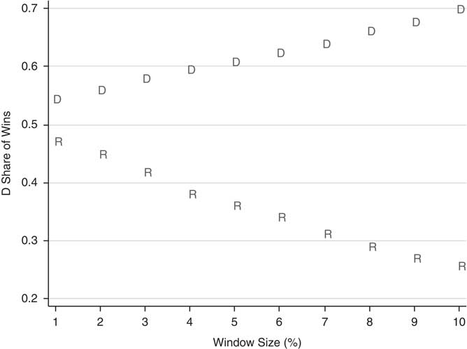
Fig. 3 Share of wins for Democrats (Republicans) in close elections in Democratic- (Republican-) leaning states as a function of definition of close elections (δ). Note: D=Democratic-leaning states; R=Republican-leaning states.

As predicted by the simple model above, the Democrats win more than 50 percent of close races in the Democratic-leaning states, and this percentage grows substantially as the window used to define close elections grows. There is a similar pattern of Republican advantage in close races in Republican-leaning states. For δ ≥ 2%, the differences between the Democratic-leaning and Republican-leaning states are quite large and statistically significant.

We now turn to the question of whether this imbalance can be attributed more to party control of the governorship, as posited by Grimmer et al. (Reference Grimmer, Hersh, Feinstein and Carpenter2011), or simply to the partisan leaning of the state, as the model above predicts. Consider the following specification:

(5) $$G_{i} =\phi _{0} {\plus}\phi _{1} D_{i} {\plus}\nu _{i} ,$$

where the dependent variable G _i =1 if the Democrats control the governorship in the state where race i is held at the time of the election, and G _i =0 if the Republicans control the governorship; D _i =1 if the Democratic candidate wins race i and D _i =0 if the Republican candidate wins. If “close” elections are randomly assigned, then we expect ϕ ₁ to be zero even in Equation 15. However, if the governor is able to help his or her co-partisans win close elections, then we would expect ϕ ₁>0.

The analysis above suggests that the imbalance due to the partisanship of the state could be corrected with more information about the forcing variable or by directly incorporating information about the partisanship of the state, as in the following two specifications:

(6) $$G_{i} =\phi _{0} {\plus}\phi _{1} D_{i} {\plus}f(V_{i} ){\plus}\nu _{i} $$

(7) $$G_{i} =\phi _{0} {\plus}\phi _{1} D_{i} {\plus}\phi _{2} P_{i} {\plus}\nu _{i} ,$$

where V _i is the share of votes received by the Democratic candidate in race i, and P _i is a measure of the partisanship of voters in the state where race i is held at (or at least near) the time of the election. The notation f (V _i ) simply denotes the possibility of using flexible functional forms in controlling for V _i , including splines, polynomials and split polynomials. P _i =1 when a state year is “Democratic leaning,” and P _i =0 when a state year is “Republican leaning.” We estimate the equations above limiting the sample to the set of “close” races, in which the winner’s vote percentage is below (50+δ) percent, for δ∈{1,2,3,4,5}.

In Table 2a we present our estimates of Equations 5–7 for the period 1876–1945. In this earlier period, we suspect that there was more partisan imbalance. The rows of the top panel show the point estimate of the main parameter of interest, ϕ ₁, as well as its standard error, in parentheses. The rows of the bottom panel show estimates of Equations 5 and 7 for the subsample of observations for which we have estimates of P. In all cases, the standard errors are corrected for heteroskedasticity using the Huber-White sandwich estimator.

Table 2a Imbalance in Gubernatorial Control in Analysis of Statewide Races, 1876–1945

Note: the dependent variable is that the sitting governor is Democratic. The top four panels show the point estimates of the coefficient on Democratic Win. Robust standard errors in parentheses. Number of observations in brackets. The term in italics is the bandwidth chosen by the Imbens and Kalyanaraman procedure.

The top row (called “Baseline”) uses all available data and provides estimates of ϕ ₁ when D is the only independent variable. The results in this panel show that the imbalance observed in Grimmer et al. (Reference Grimmer, Hersh, Feinstein and Carpenter2011) for the US House elections is also present for statewide office elections, at least for wide-enough windows around the 50 percent threshold. More specifically, when the Democratic candidate wins a given statewide race—even by a relatively close margin—the Democrats are more likely to be in control of the governorship at the time of the election. The estimated “effect” is large and statistically significant at the 5 percent level for δ ≥3.

Rows 2 and 3 show the estimates after employing one of the two standard methods for addressing the concern about partisan imbalance around the RDD threshold. In the second row we include a third-order polynomial control function, and in the third row we include a simple linear control function. Both methods appear to work well. The point estimates of ϕ ₁ are much smaller than those in the top panel—in fact, the signs are almost all negative—and statistically indistinguishable from zero. That is, the “imbalance” with respect to the party of the sitting governor disappears once we include any of the control functions.

Rows 4 and 5 present the estimates of Equation 7, with D and P both included as independent variables. As discussed above, directly incorporating information about the partisanship of the state would be one way to address our concerns about partisan imbalance around the threshold. Although we are using a relatively crude measure of P, our estimates for ϕ ₁ are closer to zero than the baseline estimates in the first row. Also, $$\hat{\phi }_{1} $$ is not statistically significant at the 5 percent level in any of the windows. The estimates of ϕ ₂ are uniformly large, stable and statistically significant for all values of δ.

The last row shows that the differences in $$\hat{\phi }_{1} $$ between Rows 1 and 4 are not simply reflecting the sample of states for which we measure P. We present the baseline results for this sample of states in the fifth row, and the bias appears in the 5 percentage point window.

Table 2b presents our estimates of Equations 5–7 for the period 1946–2010. Again, we would expect the problem of imbalance to be less severe, since many states were considered to be competitive during this period. In the first panel of Table 2b, we see that the imbalance is only statistically significant in the 5 percentage point window. Again, the imbalance is not statistically significant for any of the windows using the polynomial control or linear control. The results in the fourth and fifth rows provide evidence that the results are statistically insignificant at the 5 percent level for δ<5 when a measure of P is directly included. The imbalance still appears to be present in the 5 percentage point window.

Table 2b Imbalance in Gubernatorial Control in Analysis of Statewide Races, 1946–2010

Note: the dependent variable is that the sitting governor is Democratic. The top four panels show the point estimates of the coefficient on Democratic Win. Robust standard errors in parentheses. Number of observations in brackets. The term in italics is the bandwidth chosen by the Imbens and Kalyanaraman procedure.

Implications for Estimates of the Party Incumbency Advantage

We can now demonstrate how party incumbency advantage estimates vary when the three methods for accounting for the partisan imbalance are (or are not) included in the analysis. We use the same specification as in Equations 5, 6 and 7, but now the dependent variable is whether the Democrats win in the next election. Thus ϕ ₁ is now the party incumbency advantage that is estimated in Lee (Reference Lee2008).

We begin by examining the period from 1876–1945. Previous research finds that the incumbency advantage in this period was small.Footnote ¹² But as noted above, there was substantial partisan imbalance in many states, which was correlated with the partisanship of the governor. The baseline coefficient estimates in the top row of Table 3a illustrate the potential bias that arises from partisan imbalance. The magnitude of the party incumbency advantage increases when the size of the window increases, from 1 percent in the 1 percentage point window to 3.7 percent in the 5 percentage point window. The baseline effect of incumbency on the probability of winning, which is presented in the fourth row, increases from 0.082 to 0.256. The steady increase in the estimates is consistent with what we would expect to happen due to the partisan imbalance around the RDD threshold.

Table 3a Party Incumbency Advantage in Statewide Races, 1876−1945

Note: the top four panels show the point estimates of the coefficient on Democratic Win. Robust standard errors in parentheses. Number of observations in brackets. The term in italics is the bandwidth chosen by the Imbens and Kalyanaraman procedure.

Rows 2, 3, 5 and 6 of Table 3a show that the estimated incumbency advantage is essentially zero and not statistically significant once we incorporate the polynomial or local linear control function. Note that the estimates are stable as we change the specification window, which is what we expect when the methods are successful in adjusting for the variation in partisan imbalance across the different windows.

A number of studies have documented the growth of the incumbency advantage during the second half of the 20^th century. In Table 3b we present our estimates of the party incumbency advantage for the period 1946–2010. When we use the baseline specification, the results in Panel 1 demonstrate a steady increase in the estimated party incumbency advantage, from 5.6 percent in the 1 percentage point window to 6.9 percent in the 5 percentage point window. We observe a similar pattern for the relationship between incumbency and the probability of winning the next election. The estimated effect of incumbency on the probability of winning moves from 0.315 to 0.375. The patterns in these baseline estimates are consistent with our concern that the party incumbency advantage estimated using an RDD is biased due to partisan imbalance around the threshold.

Table 3b Party Incumbency Advantage in Statewide Races, 1946–2010

Note: the top four panels show the point estimates of the coefficient on Democratic Win. Robust standard errors in parentheses. Number of observations in brackets. The term in italics is the bandwidth chosen by the Imbens and Kalyanaraman procedure.

As with the estimates of the party incumbency advantage in the earlier period, once we incorporate the polynomial or local linear control, the estimates of the party incumbency advantage do not increase steadily with the size of the window, but are relatively stable across windows.

Appendix Tables A.1a and A.1b replicate the analyses in Tables 3a and 3b for US House elections. The pattern of coefficients in the baseline specifications in these tables is also consistent with what we would expect when there is partisan imbalance around the threshold. The coefficient estimates after including local linear or polynomial control functions are closer to the estimates obtained by other researchers using different research designs. Also, they do not increase monotonically with the size of the close election window, but are stable across windows.