2.1. Formulation of the problem

We consider an unbounded, plane and turbulent jet (Giger, Dracos & Jirka Reference Giger, Dracos and Jirka1991; Jirka Reference Jirka1994), released in an ambient flow with the same temperature, salinity and density, with the presence of obstructions and a background rotation $\varOmega$. It is appropriate to specify that, assuming $\lambda$ the latitude and $\omega$ the rotation rate of the Earth, the Coriolis parameter is given by $2\omega \sin \lambda =2 \varOmega$. The top and bottom boundaries being assumed far from the jet, conventional Ekman theory is neglected. The origin of the coordinate system is at the centre of the jet release nozzle, the $x$ axis is the curvilinear axis coinciding with the jet main axis, the $y$ axis is normal to the $x$ axis (oriented in the direction opposed to that of jet radius of curvature $r$) and the $z$ axis is vertical and parallel to the rotation axis (as depicted in figure 3).

Figure 3. Sketch of a plane jet. (a) Plan view of the jet with a clockwise rotation. (b) Typical velocity profiles at the nozzle exit (on the left) and in the zone of established flow (on the right).

In the case of a plane turbulent jet issuing into an ambient fluid at rest with the presence of the Coriolis force and a cylinder array (figure 3), the Reynolds equations of motions are

(2.1)\begin{align} &\frac{\partial u}{\partial t}+u\frac{\partial u}{\partial x}+v\frac{\partial u}{\partial y}+w\frac{\partial u}{\partial z}-2\varOmega v\nonumber\\ &\quad ={-}\frac{1}{\rho}\frac{\partial p}{\partial x}+\nu\left(\frac{\partial^{2}u}{\partial x^{2}}+\frac{\partial^{2}u}{\partial y^{2}} +\frac{\partial^{2}u}{\partial z^{2}}\right)-\left(\frac{\partial\overline{u^{\prime 2}}}{\partial x}+\frac{\partial\overline{u^{\prime} v^{\prime}}}{\partial y}+\frac{\partial\overline{u^{\prime} w^{\prime}}}{\partial z}\right)-\frac{1}{\rho}D_x, \end{align}

(2.2)\begin{align} &\frac{\partial v}{\partial t}+\frac{U_b^{2}}{r}+u\frac{\partial v}{\partial x}+v\frac{\partial v}{\partial y}+w\frac{\partial v}{\partial z}+2\varOmega u\nonumber\\ &\quad ={-}\frac{1}{\rho}\frac{\partial p}{\partial y}+\nu\left(\frac{\partial^{2}v}{\partial x^{2}}+\frac{\partial^{2}v}{\partial y^{2}}+\frac{\partial^{2}v}{\partial z^{2}}\right)-\left(\frac{\partial\overline{u^{\prime} v^{\prime}}}{\partial x}+\frac{\partial\overline{v^{\prime 2}}}{\partial y}+\frac{\partial\overline{v^{\prime} w^{\prime}}}{\partial z}\right)-\frac{1}{\rho}D_y, \end{align}

(2.3)\begin{align} &\frac{\partial w}{\partial t}+u\frac{\partial w}{\partial x}+v\frac{\partial w}{\partial y}+w\frac{\partial w}{\partial z}\nonumber\\ &\quad ={-}\frac{1}{\rho}\frac{\partial p}{\partial z}+\nu\left(\frac{\partial^{2}w}{\partial x^{2}}+\frac{\partial^{2}w}{\partial y^{2}}+\frac{\partial^{2}w}{\partial z^{2}}\right)-\left(\frac{\partial\overline{u^{\prime} w^{\prime}}}{\partial x}+\frac{\partial\overline{v^{\prime} w^{\prime}}}{\partial y}+\frac{\partial\overline{w^{\prime 2}}}{\partial z}\right)-\frac{1}{\rho}D_z, \end{align}

where $u$, $v$ and $w$ and $u^{\prime }$, $v^{\prime }$ and $w^{\prime }$ are the time-averaged and fluctuating velocity components in the $x$, $y$ and $z$ directions, respectively, $p$ is the time-averaged pressure at any point, $\nu$ is the kinematic viscosity and $\rho$ is the mass density of both the jet and ambient fluid. The centripetal acceleration is $U_b^{2}/r$, with $U_b$ being the average of the longitudinal velocity in each cross-section. Furthermore, the drag forces in the $x$, $y$ and $z$ directions, i.e. the resistance due to the solid medium, sum of form and viscous drag over the stem, are $D_x$, $D_y$ and $D_z$, respectively; $t$ is the time variable and the overbar represents a time-average operator.

The continuity equation is

(2.4)\begin{equation} \frac{\partial u}{\partial x}+\frac{\partial v}{\partial y}+\frac{\partial w}{\partial z}=0. \end{equation}

The relevant dimensionless parameters of the analysed flow are the Rossby number $R_o$ and the Reynolds number $R_e$, defined as

(2.5a,b)\begin{equation} R_o=\frac{U_0}{\varOmega L_x} ,\quad R_{e}=\frac{U_0 b_0}{\nu}, \end{equation}

where $L_x$ is the jet-like longitudinal length scale and $U_0$ is the velocity at the jet nozzle (figure 3b).

It is worth noting that atmospheric and oceanographic flows can be considered as shallow with horizontal length scales much larger than their vertical length scales. Therefore they could be described using the shallow water equations. The Rossby number, which characterizes the strength of inertia compared to the strength of the Coriolis force, is equal to zero or is very small in the case of a geostrophic flow. In our quasi-geostrophic jet-like flow, the Rossby number is of order 1, so that the Coriolis and inertial forces are of similar magnitude. Below we consider only the zone of established flow (at $x>x_0$), where the longitudinal velocity distribution in each cross-section, i.e. the distribution of the u-velocity in the radial direction, has the same well-known Gaussian shape shown in figure 3 (Pope Reference Pope2000). As shown in figure 3(b), at each cross-section the maximum longitudinal velocity component is $u_m$ and $b$ is the typical length scale, which is generally assumed as the distance from the jet centreline where the longitudinal velocity is $u=u_m/e$, with $e$ being the Euler number, whose value is equal to $b_0$ at the jet origin. In the present model we consider the case of unbounded plane jets issuing into an ambient flow with a regular square array of emergent cylinders of uniform diameter $d$ and distance $s$ (figure 4). Another key parameter of the cylinder array used in the present paper is the frontal area per unit volume of the obstructions $a=nd$, which is equal to $d/s^{2}$ in the case of a periodic square array, where $n$ is the number of elements per unit planar area (Nepf Reference Nepf1999). The local variations of the velocity profiles detected in flows with obstacles (Ben Meftah & Mossa Reference Ben Meftah and Mossa2016) are not considered here. However, the envelope cross-section velocity profile is taken into account to evaluate the effects of the presence of obstacles on the entire velocity profile.

Figure 4. Sketch of the analysed plane jet. (a) Unbounded jet-like flow. (b) Plan view of the jet with the cylinder array.

The effect of obstructions is considered using the drag coefficient $C_D$ in the drag terms. As shown by Nepf (Reference Nepf1999), various resistance laws of drag for flow in porous media can be derived. Particularly, in obstructed free-surface flows, the following quadratic form can be assumed:

(2.6)\begin{equation} D_i=\tfrac{1}{2}\rho\, C_Da|u_i|u_i, \end{equation}

with $i=x,y,z$ (Kaimal & Finnigan Reference Kaimal and Finnigan1994). Since the flow is quasi-two-dimensional, we can approximate that $w=0$, $\partial /\partial z =0$, $\overline {u^{\prime } w^{\prime }}=0$ and $\overline {v^{\prime } w^{\prime }}=0$, and consider the mean flow as steady, $\partial /\partial t =0$. Furthermore, $u$ is generally much larger than $v$ in a large portion of the jet and velocity and stress gradients in the $y$ direction are much larger. Therefore, (2.1) and (2.2) become

(2.7)$$\begin{gather} u\frac{\partial u}{\partial x}+v\frac{\partial u}{\partial y}-2\varOmega v={-}\frac{1}{\rho} \frac{\partial p}{\partial x}+\nu\frac{\partial^{2}u}{\partial y^{2}}-\frac{\partial\overline{u^{\prime 2}}}{\partial x}-\frac{\partial\overline{u^{\prime} v^{\prime}}}{\partial y}-\frac{1}{\rho}D_x, \end{gather}$$

(2.8)$$\begin{gather}0={-}\frac{1}{\rho}\frac{\partial p}{\partial y}-\frac{\partial\overline{v^{\prime 2}}}{\partial y}-\frac{1}{\rho}D_y-2\varOmega u-\frac{U_b^{2}}{r}. \end{gather}$$

Assuming $\mathscr {B}$ as the nominal outer boundary of the jet where $u$ is close to 0, it is possible to write

(2.9)\begin{equation} \mathscr{B} = \mathscr{C}_b b, \end{equation}

where $\mathscr {C}_b$ is a constant. Integrating (2.8), with $P$ as the pressure outside the jet and assuming the radius of curvature sufficiently large to have symmetric/antisymmetric conditions for both sides of the jet, we get

(2.10)\begin{equation} p=P-\rho\overline{v^{\prime 2}}-\int_{0}^{\mathscr{B}}({2\rho\varOmega u+D}_y)\,{\textrm{d} y}. \end{equation}

Differentiating (2.10) with respect to $x$ and using it in (2.7), we get

(2.11)\begin{align} u\frac{\partial u}{\partial x}+v\frac{\partial u}{\partial y}-2\varOmega v&={-}\frac{1}{\rho}\frac{\textrm{d}P}{\textrm{d}\,x}+\nu\frac{\partial^{2}u}{\partial y^{2}}-\frac{\partial\overline{u^{\prime} v^{\prime}}}{\partial y}-\frac{\partial}{\partial x}(\overline{u^{\prime 2}}-\overline{v^{\prime 2}})\nonumber\\ &\quad -\frac{1}{\rho}\left(D_x+\frac{\textrm{d}}{\textrm{d}\,x}\int_{0}^{\mathscr{B}}{D_y\,\textrm{d}y+\frac{\textrm{d}}{\textrm{d}\,x}\int_{0}^{\mathscr{B}}2\rho\varOmega u\,\textrm{d}y}\right). \end{align}

As shown by Mossa et al. (Reference Mossa, Ben Meftah, De Serio and Nepf2017) and De Serio et al. (Reference De Serio, Ben Meftah, Mossa and Termini2018), assuming that

(2.12)\begin{equation} D_x \gg\frac{\textrm{d}}{\textrm{d}\,x}\int_{0}^{\mathscr{B}}{D_y\,\textrm{d}y} \end{equation}

we obtain

(2.13)\begin{align} u\frac{\partial u}{\partial x}+v\frac{\partial u}{\partial y}-2\varOmega v&={-}\frac{1}{\rho}\frac{\textrm{d}P}{\textrm{d}\,x}+\nu\frac{\partial^{2}u}{\partial y^{2}}-\frac{\partial\overline{u^{\prime} v^{\prime}}}{\partial y}-\frac{1}{\rho}D_x-2\varOmega\left(\frac{\textrm{d}}{\textrm{d}\,x}\int_{0}^{\mathscr{B}}u\,\textrm{d}y\right)\nonumber\\ &={-}\frac{1}{\rho}\frac{\textrm{d}P}{\textrm{d}\,x}+\nu\frac{\partial^{2}u}{\partial y^{2}}-\frac{\partial\overline{u^{\prime} v^{\prime}}}{\partial y}-\frac{1}{\rho}D_x-2\varOmega v_e, \end{align}

where

(2.14)\begin{equation} v_e=\frac{\textrm{d}}{\textrm{d}\,x}\int_{0}^{\mathscr{B}}u\,\textrm{d}y \end{equation}

is the so-called entrainment velocity, which can be written as

(2.15)\begin{equation} v_e=\alpha_e u_m, \end{equation}

with $\alpha _e$ the entrainment/detrainment coefficient (Rajaratnam Reference Rajaratnam1976; Mossa & De Serio Reference Mossa and De Serio2016). Observing that the laminar and turbulent stresses are, respectively,

(2.16)\begin{equation} \left\{ \begin{aligned} & \tau_l=\mu\dfrac{\partial u}{\partial y}\\ & \tau_t={-}\rho\overline{u^{\prime} v^{\prime}} \end{aligned} \right. \end{equation}

and considering that $\tau _t$ is much larger than $\tau _l$ for the flows here considered and the gradient of pressure is null along the horizontal trajectories in geostrophic flows, which means the trajectories must take place along isochoric lines, we get

(2.17)\begin{equation} u\frac{\partial u}{\partial x}+v\frac{\partial u}{\partial y}-2\varOmega v=\frac{1}{\rho}\frac{\partial\tau_t}{\partial y}-\frac{1}{\rho}D_x-2\varOmega v_e. \end{equation}

Integration of (2.17) gives

(2.18)\begin{equation} \rho\int_{0}^{\mathscr{B}}{u\frac{\partial u}{\partial x}{\textrm{d} y}}+\rho\int_{0}^{\mathscr{B}}{v\frac{\partial u}{\partial y}{\textrm{d} y}}-\int_{0}^{\mathscr{B}}{\frac{\partial\tau_t}{\partial y}{\textrm{d} y}}={-}\int_{0}^{\mathscr{B}}\left(D_x+2\rho\varOmega v_e-2\rho\varOmega v\right){\textrm{d} y}, \end{equation}

which becomes

(2.19)\begin{equation} \frac{1}{2}\frac{\textrm{d}}{\textrm{d}\,x}\int_{0}^{\mathscr{B}}{\rho u^{2}\,\textrm{d}y}+\rho\left(\left|uv\right|_{y=0}^{y=\mathscr{B}}-\int_{0}^{\mathscr{B}}{u\frac{\partial v}{\partial y}{\textrm{d}y}}\right)={-}\int_{0}^{\mathscr{B}}\left(D_x+2\rho\varOmega v_e-2\rho\varOmega v\right){\textrm{d} y}. \end{equation}

Using the continuity equation (2.4), we obtain

(2.20)\begin{equation} \frac{\textrm{d}}{\textrm{d}\,x}\int_{0}^{\mathscr{B}}{\rho u^{2}\,\textrm{d}y}={-}\int_{0}^{\mathscr{B}} \left(D_x+2\rho\varOmega v_e-2\rho\varOmega v\right){\textrm{d} y}. \end{equation}

If we write

(2.21)\begin{equation} D_x=\tfrac{1}{2}\rho\,C_Dau^{2} \end{equation}

we obtain that

(2.22)\begin{equation} \frac{\textrm{d} \mathscr{M}\left(x\right)}{\textrm{d}\,x}=\frac{\textrm{d}}{\textrm{d}\,x} \int_{0}^{\mathscr{B}}{ u^{2}\,\textrm{d}y}={-}\frac{1}{2}C_Da\int_{0}^{\mathscr{B}}{ u^{2}\,\textrm{d}y-2 \varOmega v_e\mathscr{B}}+\int_{0}^{\mathscr{B}} 2 \varOmega v\,\textrm{d}y, \end{equation}

where $\mathscr {M}(x)$ is half the kinematic momentum flux in each cross-section. It is reasonable to assume that the trend of the $v$-velocity component along $y$ should be antisymmetric with respect to the jet axis (Goertler Reference Goertler1942). The last two terms of the right-hand side of (2.22) are overall responsible for a momentum decrease due to the jet rotation and, using a scale analysis (Tennekes & Lumley Reference Tennekes and Lumley1972), they are similar. Therefore, it is reasonable to write that

(2.23)\begin{equation} -2\varOmega v_e\mathscr{B}+\int_{0}^{\mathscr{B}}\left(2\varOmega v\right){\textrm{d} y}={-}2 \chi_{ve}\varOmega v_e\mathscr{B}, \end{equation}

where $\chi _{ve}$ is an empirical coefficient.

2.2. Velocity and cross-length scales

In the zone of established flow of a turbulent plane jet, the velocity distribution is similar (Rajaratnam Reference Rajaratnam1976; Barile et al. Reference Barile, De Padova, Mossa and Sibilla2020), so that

(2.24)\begin{equation} \frac{u}{u_m}=f\left(\eta\right), \end{equation}

with $\eta =y/b$.

Assuming power forms for $u_m$ and $b$:

(2.25)\begin{equation} \left\{\begin{aligned} & b \propto x^{\phi} \Rightarrow b=\mathscr {F}_1x^{\phi} \\ & u_m \propto x^{\psi} \Rightarrow u_m=\mathscr{F}_2x^{\psi} , \end{aligned} \right. \end{equation}

where $\phi$ and $\psi$ are unknown exponents to be found. Equation (2.25) is valid for the zone of established flow.

By the change of variable $y = \eta /b$, since for $y = 0$ we have $\eta = 0$, and for $y = \mathscr {B}$ we get $\eta = y/b = \mathscr {B}/b = \mathscr {C}_b$, it follows that

(2.26)\begin{equation} \frac{\textrm{d}}{\textrm{d}\,x}\int_{0}^{\mathscr{C}_b}{u_m^{2}f^{2}b\,\textrm{d}\eta}={-}\frac{1}{2}C_Da\int_{0}^{\mathscr{C}_b}{ u_m^{2}f^{2}b\,\textrm{d}\eta-2 \varOmega \chi_{ve} v_e\mathscr{B}} \end{equation}

or, analogously,

(2.27)\begin{equation} \frac{\textrm{d}}{\textrm{d}\,x}\left( u_m^{2}b\int_{0}^{\mathscr{C}_b}{f^{2}\,\textrm{d}\eta}\right)={-}\frac{1}{2}C_Dau_m^{2}b\int_{0}^{\mathscr{C}_b}{ f^{2}\,\textrm{d}\eta-2\varOmega \chi_{ve} v_e\mathscr{B}}. \end{equation}

Considering that

(2.28)\begin{equation} \int_{0}^{\mathscr{C}_b}{f^{2}\,\textrm{d}\eta}=\textrm{const}., \end{equation}

equation (2.27) can be rewritten as

(2.29)\begin{equation} \frac{\textrm{d}}{\textrm{d}\,x}(u_m^{2}b)={-}\frac{1}{2}C_Dabu_m^{2}-\frac{2\varOmega \chi_{ve} v_e\mathscr{B}}{\displaystyle\int_{0}^{\mathscr{C}_b}{f^{2}\,\textrm{d}\eta}}, \end{equation}

i.e.

(2.30)\begin{equation} 2\psi+\phi={-}\frac{1}{2}C_Da x-\frac{2\varOmega \chi_{ve} \alpha_e \mathscr{C}_b x^{1-\psi}}{\displaystyle\int_{0}^{\mathscr{C}_b}{f^{2}\,\textrm{d}\eta}}. \end{equation}

From dimensional considerations it is possible to write that

(2.31)\begin{equation} \frac{\tau}{\rho u_m^{2}}=g\left(\eta\right). \end{equation}

Considering (2.24) and (2.31), denoting the derivatives with a prime symbol, we have

(2.32a–d)\begin{equation} f^{\prime}=\frac{\textrm{d}f}{\textrm{d}\eta}, \quad g^{\prime}=\frac{\textrm{d}g}{\textrm{d}\eta},\quad b^{\prime}=\frac{\textrm{d}b}{\textrm{d}\,x},\quad u^{\prime}_m=\frac{\textrm{d}u_m}{\textrm{d}\,x}, \end{equation}

and therefore we obtain

(2.33)$$\begin{gather} u\frac{\partial u}{\partial x}=u_mu^{\prime}_mf^{2}-\frac{u_m^{2}b^{\prime}}{b}\eta\ ff^{\prime}, \end{gather}$$

(2.34)$$\begin{gather}v\frac{\partial u}{\partial y}=\frac{u_m^{2}b^{\prime}}{b}\left(\eta \,ff^{\prime}-f^{\prime}\int_{0}^{\eta}f\,\textrm{d}\eta\right)-u_mu^{\prime}_m\,f^{\prime}\int_{0}^{\eta}\,f\,\textrm{d}\eta, \end{gather}$$

(2.35)$$\begin{gather}\frac{1}{\rho}\frac{\partial\tau}{\partial y}=\frac{u_m^{2}}{b}g^{\prime}, \end{gather}$$

(2.36)$$\begin{gather}-\frac{1}{\rho}D_x={-}\frac{1}{2}C_Dau_m^{2}\,f^{2}, \end{gather}$$

(2.37)$$\begin{gather}-2\varOmega v_e={-}2\varOmega\alpha_eu_m. \end{gather}$$

Substituting (2.33), (2.34), (2.35) and (2.36) into (2.17), we obtain

(2.38)\begin{align} g^{\prime}&=\frac{bu\prime_m}{u_m}\left(f^{2}-f^{\prime}\int_{0}^{\eta}f\,\textrm{d}\eta\right)-b^{\prime}\left(\eta\, f^{\prime}-\eta \,f\ f^{\prime}+f^{\prime}\int_{0}^{\eta}f\,\textrm{d}\eta\right)\nonumber\\ &\quad +\frac{1}{2}C_Dabf^{2}+2\chi_{ve}\varOmega\alpha_eu_m. \end{align}

Since $g^{\prime }$ is a function of only $\eta$, the right-hand side should also be a function of only $\eta$ (Mossa et al. Reference Mossa, Ben Meftah, De Serio and Nepf2017; Barile et al. Reference Barile, De Padova, Mossa and Sibilla2020). Particularly, from the first two terms on the right-hand side, it is possible to write

(2.39)\begin{equation} \left\{\begin{aligned} & \frac{bu^{\prime}_m}{u_m}\propto x^{\phi-1}\\ & b^{\prime}\propto x^{\phi-1}, \end{aligned} \right. \end{equation}

and therefore

(2.40)\begin{equation} \phi=1, \end{equation}

i.e.

(2.41)\begin{equation} b=\mathscr {F}_1\cdot x. \end{equation}

In the present study we will consider jets with

(2.42)\begin{equation} b=\mathscr{O}\left(n\cdot s\right), \end{equation}

with $n=\mathscr {O}(10 - 10^{2})$. In other words, referring to figure 4(b), we are considering the case where $d/s=\mathscr {O}(10^{-1} - 1)$, $b/d=\mathscr {O}(10 - 10^{2})$, $b/s=\mathscr {O}(10 - 10^{2})$, such as that shown by Mossa et al. (Reference Mossa, Ben Meftah, De Serio and Nepf2017).

Therefore, it is possible to write

(2.43)\begin{equation} b=\mathscr {F}_1x^{\phi} =\mathscr{O}\left(\left(10\div 100\right)\cdot s\right). \end{equation}

The order of magnitude of $b$ changes when it becomes

(2.44)\begin{equation} 10b=10\mathscr {F}_1x^ \phi=\mathscr{O}\left(\left(100\div 1000\right)\cdot s\right), \end{equation}

i.e. when $x^{\phi }$ increases by an order of magnitude or more. Therefore, $b$ has the same order of magnitude between two values of $x$, i.e. from $x_1$ to $x_2>x_1$, when

(2.45)\begin{equation} \frac{x_2^{\phi}}{x_1^{\phi}}<\mathscr{O}\left(10\right). \end{equation}

Since in the analysed case $\phi =1$, it is possible to write that

(2.46)\begin{equation} x_1,x_2=\mathscr{O}\left(n\cdot s\right)\quad\mathrm{with}\ n\geqslant 10 - 100. \end{equation}

Furthermore, the rotation rate of the Earth $\varOmega$ is equal to $7.2921\times 10^{- 5}\ \textrm {rad}\ \textrm {s}^{-1}$. It can be calculated as $2{\rm \pi} /T\ \textrm {rad}\ \textrm {s}^{-1}$, where $T$ is the rotation period of the Earth which is one sidereal day.

Therefore, along a longitudinal distance between $x_1$ and $x_2$ satisfying (2.43), equation (2.39) becomes

(2.47)\begin{align} g^{\prime}&\approx\frac{bu^{\prime}_m}{u_m}\left(f^{2}-f^{\prime}\int_{0}^{\eta}f\,\textrm{d}\eta\right)\nonumber\\ &\quad -b^{\prime}\left(\eta f^{\prime}-\eta f\ f^{\prime}+f^{\prime}\int_{0}^{\eta}f\,\textrm{d}\eta\right)+\frac{1}{2}C_D\frac{d}{s^{2}}nsf^{2}+O\left({10}^{{-}5}\right), \end{align}

where the third term of the right-hand side can be considered approximately constant in the described limits. With these considerations in mind and using (2.39) and (2.30), it is possible to conclude that

(2.48)\begin{equation} \left\{ \begin{aligned} & \phi =\mathscr{O}\left(1\right) \\ & \psi =\mathscr{O}\left(-\frac{1}{2}\right)-\frac{1}{4}C_Dax=\mathscr{O}\left(-\frac{1}{2}\right)-\frac{1}{4}C_D\frac{d}{s^{2}}x=C_p\left(-\frac{1}{2}-\frac{1}{4}C_D\frac{d}{s^{2}}x\right), \end{aligned} \right. \end{equation}

where, therefore, $C_p$ must have an order of magnitude of 1.

The $x$ coordinate was previously considered as a curvilinear one. We analyse the theoretical model description of the jet each time addressing a relatively small range $x=[x_1, x_2]>x_0$ defined by the order of magnitude of $b$. With the change of order of magnitude of $b$, as we move along the jet axis, a new region is defined. Figure 5 shows the described divisions into regions, where $X$ and $Y$ are the axes of a Cartesian coordinate system (Barile et al. Reference Barile, De Padova, Mossa and Sibilla2020).

Figure 5. Regions of the jet where, as a fist approximation, the order of magnitude of $b$ is constant.

This means that making the laws of $b$ and $u_m$ (equation (2.25)) dimensionless, we have

(2.49)$$\begin{gather} \frac{b}{b_0}=C_1\left(\frac{x}{x_0}\right)^{\phi}+C_2, \end{gather}$$

(2.50)$$\begin{gather}\frac{u_m}{U_0}=C_3\left(\frac{x^{\psi}}{{x_0}^{\psi_0}}\right)+C_4, \end{gather}$$

where $\psi _0$ is the value of $\psi$ for $x=x_0$. It is reasonable to assume that the coefficients are a function of the range of $x$. In other words, the structures of the laws of $b$ and $u_m$ remain the same, but the coefficients can vary between the ranges and must be obtained from experiments.

2.3. The momentum flux deficit

Considering (2.9), (2.15) and (2.25), we have the following equation in terms of scale analysis:

(2.51)\begin{equation} -2 \chi_{ve}\varOmega v_e\mathscr{B}={-}2\varOmega \chi_{ve} \mathscr{C}_b \mathscr{F}_1 x^{\phi} \alpha_e \mathscr{F}_2 x^{\psi}. \end{equation}

Therefore, integrating (2.22), where the density $\rho$ is not present, since we do not have variation of density, we have

(2.52)\begin{equation} \mathscr{M}=c_1 \textrm{e}^{-({1}/{2}) C_D a x} - \int 2 \varOmega \chi_{ve} \mathscr{C}_b \mathscr{F}_1 x^{\phi} \alpha_e \mathscr{F}_2 x^{\psi} \,{\textrm{d}\,x}. \end{equation}

Making (2.52) non-dimensional for reasons that will be clear afterwards, (2.52) becomes

(2.53)\begin{equation} \mathfrak{M}=\mathfrak{c}_1 \textrm{e}^{-({1}/{2}) C_D \mathfrak{a}\mathfrak{x}} -\int 2\mathfrak{O} \chi_{ve} \mathscr{C}_b \mathfrak{F}_1 \mathfrak{x}^{\phi} \alpha_e \mathfrak{F}_2 \mathfrak{x}^{\psi} \,\textrm{d} \mathfrak{x}, \end{equation}

where

(2.54a–g)\begin{equation} \left.\begin{gathered} \mathfrak{M}=\frac{\mathscr{M}}{U_0^{2}x_0}, \quad\mathfrak{x}=\frac{x}{x_0},\quad \mathfrak{a}=a x_0, \quad\mathfrak{c}_1=\frac{c_1}{U_0^{2}x_0},\quad \mathfrak{O}=\frac{\varOmega}{U_0 x_0}, \\ \mathfrak{F}_1=\frac{\mathscr{F}_1}{x_0}, \quad\mathfrak{F}_2=\frac{\mathscr{F}_2}{U_0} \end{gathered}\right\} \end{equation}

are all dimensionless. Considering (2.54a–g), the second term of the right-hand side of (2.52) can be rewritten as follows:

(2.55)\begin{equation} \int -\mathfrak{C}_1 \mathfrak{x}^{0.5-\mathfrak{C}_2\mathfrak{x}} \,\textrm{d}\mathfrak{x}. \end{equation}

Integral (2.55) does not have a solution, but we could expand the integrating function. Therefore, we obtain

(2.56)\begin{align} \mathfrak{C}_1 \mathfrak{x} ^{0.5-\mathfrak{C}_2 \mathfrak{x}} & =\mathfrak{x}^{0.5} \sum_{i=0}^{n} \frac{({-}1)^{n}}{n!}\mathfrak{C}_1 \mathfrak{C}_2^{n} \log^{n}(\mathfrak{x})\mathfrak{x}^{n}\nonumber\\ &=\mathfrak{x}^{0.5} \left(\mathfrak{C}_1 - \mathfrak{C}_1\mathfrak{C}_2 \log (\mathfrak{x}) \mathfrak{x} +\mathscr{O}(\mathfrak{x})^{2}\right). \end{align}

Using a first-order approximation, (2.55) becomes

(2.57)\begin{align} &\int -\mathfrak{x}^{0.5} \left(\mathfrak{C}_1 - \mathfrak{C}_1\mathfrak{C}_2 \log (\mathfrak{x}) \mathfrak{x} \right) \textrm{d}\mathfrak{x}\nonumber\\ &\quad ={-}\frac{2}{75} \mathfrak{C}_1 \mathfrak{x}^{{3}/{2}} \left( 6 \mathfrak{C}_2 \mathfrak{x} -15 \mathfrak{C}_2 \log (\mathfrak{x}) \mathfrak{x} +25 \right) + \text{const.} \end{align}

Therefore, (2.53) becomes

(2.58)\begin{equation} \mathfrak{M}=\mathfrak{c}_1 \textrm{e}^{-({1}/{2}) C_D \mathfrak{a}\mathfrak{x}} -\frac{2}{75} \mathfrak{C}_1 \mathfrak{x}^{{3}/{2}} \left( 6 \mathfrak{C}_2 \mathfrak{x} -15 \mathfrak{C}_2 \log (\mathfrak{x}) \mathfrak{x} +25 \right) + \text{const.}, \end{equation}

from which we can compute $\mathscr {M}$ using (2.54a–g). The structure of the first term of the right-hand side of (2.58) is similar to that proposed by Negretti et al. (Reference Negretti, Vignoli, Tubino and Brocchini2006) and Mossa & De Serio (Reference Mossa and De Serio2016). Equation (2.58) shows an interesting result, since a pure plane jet in a rotating system does not preserve the momentum. The momentum decrease depends both on the Rossby number, i.e. the rotation, and, in the case of obstructed flows, also on characteristics of the rods. In the case of unobstructed flows, the first term of the right-hand side of (2.58) is not present.

2.4. Jet centreline

As shown by Bradbury (Reference Bradbury1965), the sum of the first two terms of (2.8) is very small and, therefore, can be neglected, affording

(2.59)\begin{equation} 0={-}\frac{1}{\rho}D_y-2\varOmega u-\frac{U_b^{2}}{\dfrac{\textrm{d}\,x}{\textrm{d}\alpha}}, \end{equation}

where $\alpha$ is the central angle of the circumference arc to which the curvilinear segment ${\textrm{d}\,x}$ is approximated.

Analysing the trajectory where $u=u_m$, called the jet centreline, using (2.6) for $D_y$ and assuming $U_b^{2}=C_u u_m^{2}$, we have

(2.60)\begin{equation} \frac{\textrm{d}\alpha}{\textrm{d}\,x}={-}\frac{1}{\rho}\frac{\dfrac{1}{2}\rho C_DaV^{2}}{ \left(C_uu_m^{2}\right)}-2\frac{\varOmega}{C_uu_m}, \end{equation}

where $C_u$ is a dimensionless coefficient and $V$ is a velocity scale normal to the jet axis in each cross-section which can be assumed to be equal to

(2.61)\begin{equation} V^{2}=C_v\alpha_e^{2}u_m^{2}, \end{equation}

with $C_v$ an empirical coefficient. Therefore, using the second equation of (2.25) and (2.48), we obtain

(2.62)\begin{equation} \frac{\textrm{d}\alpha}{\textrm{d}\,x}={-}\frac{1}{2}\frac{C_Da{C_v\alpha}_e^{2}}{C_{u}}-2 \frac{\varOmega}{C_uC_{um}\left(\dfrac{x}{x_0}\right)^{-{1}/{2}-({1}/{4})C_D({d}/{s^{2}})x}}. \end{equation}

Equation (2.62) can be written as follows:

(2.63)\begin{equation} \frac{\textrm{d}\alpha}{\textrm{d}\left(\dfrac{x}{x_0}\right)}={-}\frac{1}{2}\frac{{x_0C}_DaC_v \alpha_e^{2}}{C_{u}}-2\frac{x_0\varOmega}{C_uC_{um}\left(\dfrac{x}{x_0}\right)^{-{1}/{2}- ({x_0}/{4})C_D({d}/{s^{2}})({x}/{x_0})}}. \end{equation}

Using $\mathfrak {x}$ defined in (2.54a–g), we get

(2.64)\begin{equation} \frac{\textrm{d}\alpha}{\textrm{d} \mathfrak{x}}={-}\frac{1}{2}\frac{{x_0C}_Da{C_v\alpha}_e^{2}}{C_{u}}-2\frac{x_0\varOmega}{C_uC_{um} \mathfrak{x}^{-{1}/{2}-({x_0}/{4})C_D({d}/{s^{2}})(\mathfrak{x})}}. \end{equation}

Rewriting (2.64) as

(2.65)\begin{equation} \frac{\textrm{d}\alpha\left(\mathfrak{x}\right)}{\textrm{d}\mathfrak{x}}={-} \mathcal{A}-\frac{\mathcal{B}}{\mathfrak{x}^{-\mathcal{C}\mathfrak{x}-0.5}}, \end{equation}

with obvious meaning of the parameters $\mathcal {A}$, $\mathcal {B}$, $\mathcal {C}$, which must be obtained from the experimental data, we get the following solution:

(2.66)\begin{equation} \alpha\left(\mathfrak{x}\right)={-}\mathcal{B}\int{\mathfrak{x}^{\mathcal{C}\mathfrak{x}+1/2}\, \textrm{d}\mathfrak{x}}-\mathcal{A}\mathfrak{x}+c_2, \end{equation}

where $c_2$ depends on the initial conditions. In the case of the absence of obstructions, i.e. $C_D=0$, (2.66) reduces to

(2.67)\begin{equation} \alpha(\mathfrak{x})={-}\tfrac{2}{3}\mathcal{B}\mathfrak{x}^{3/2}+c_2. \end{equation}

Figures 6 and 7 show typical trends of the jet axis in the absence of obstructions at increasing Rossby numbers and with obstructions at increasing $C_Dax_0$, respectively. The axes of the figures have been made non-dimensional using the length scale $L_{x0}$, defined as the maximum distance along the direction of the jet exit of the case with $R_o=1$ with $C_Dax_0=0$. They highlight the effects of both Coriolis and drag forces. For the paths in the figures we assumed that all the coefficients and variables are equal to 1, considering that the aim is only a comparison among different values of the Rossby number and the drag force.

Figure 6. Comparison among jet axes without obstructions.

Figure 7. Comparison among centre pathlines of jets with obstructions at different values of $C_Dax_0$.

3.1. Experimental apparatus

The experiments were carried out using the Coriolis rotating platform at LEGI-Grenoble, France (figure 8). In this large-scale facility, experimental runs were executed by discharging a horizontal-momentum jet in an unobstructed and obstructed fluid. In the latter case a canopy made of rigid rods was used (figure 9). The LEGI tank has a diameter of 13 m. The water depth used in the experimental runs of the present paper was equal to 0.80 m. Figure 10(a) shows a sketch of the rotating platform with the jet.

Figure 8. The Coriolis rotating platform at LEGI.

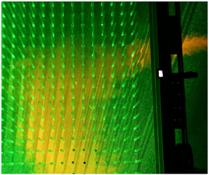
Figure 9. Experimental apparatus. (a) The stem array. (b) Jet issued in the rotating tank with stems and the PIV laser sheet.

Figure 10. Sketch of the experimental apparatus. (a) Plan view of the rotating platform with the unbounded jet-like flow. (b) Sketch of the location of jet outlet and vegetation panel in the rotating tank (plan view).

Jets were horizontally issued with a pipe, installed in the tank at a fixed depth of 0.40 m. The jet initial diameter was equal to 0.08 m (inner diameter of the pipe). A specially designed rigid cylinder array was placed in the tank for the obstructed configurations. The rigid emergent cylinders were in Plexiglas, each with a diameter equal to 0.02 m, arranged on a $2\ \textrm {m}\times 2\ \textrm {m}$ panel fixed at the bottom of the tank. The rods were manually mounted on the panel inside pre-drilled holes, thus ensuring a regular pattern with a centre-to-centre distance $s$. The panel was placed in the tank between the carriage supports, as shown in figure 10(b). The centre of the jet outlet ($O$) was 1 m from the upstream edge of the panel and 0.77 m from its external edge.

In the present paper, the runs shown in table 1 are analysed. The values of $C_D$ were obtained using the data of Nepf (Reference Nepf1999). The Reynolds number of the analysed jets, based on (2.5a,b), was equal to $91\times 10^{3}$, ensuring fully turbulent flows.

Table 1. Values of some parameters of the analysed runs.

The instantaneous measurements of the velocity field at the horizontal plane passing from the centre of the jet nozzle were assessed using a particle image velocimetry (PIV) system (figure 9b). The laser source of the PIV system was mounted in the centre of the tank. Three synchronized recording cameras were mounted on the top of the tank. A continuous YAG laser (532 nm wavelength) with a power of 25 W and a Powell prism producing a 5 mm thick laser sheet were used. The laser sheet, set in a horizontal plane, spanned an area of more than $3\ \textrm {m}\times 3 \ \textrm {m}$, with a $60^{\circ }$ opening angle. The PIV system enabled us to analyse a sufficiently large area of the rotating tank. Its acquisition frequency (33 Hz) was appropriately selected in order to avoid possible effects of disturbances of the free-surface deformations on the measurements. Furthermore, Orgasol neutrally buoyant particles with a $60\ \mathrm {\mu }\textrm {m}$ diameter were used to seed the flow. For the processing of the experimental results, custom Matlab scripts have been developed. To account for possible optical distortion due to the presence of the water–air interface, a spatial calibration was applied to all processed images.

Figures 11 and 12 show a comparison between the model and the experiential results for the length scale $b$ and velocity scale $u_m$, respectively. The comparison between theoretical and experimental results shows that the developed model describes the empirical data very well, at least for the examined experiential set-up. Table 2 lists the values of the coefficients of the theoretical laws for the analysed zones of each experimental run. The analysed zones were identified on the basis of the criteria indicated above.

Figure 11. Comparison between theoretical and experimental values of $b$.

Figure 12. Comparison between theoretical and experimental values of $u_m$.

Table 2. Values of the parameters of (2.49) and (2.50).

Figure 13 shows a comparison between the modelled and experimental values of the momentum flux. The figure shows that the momentum deficit predicted by the new model is in very good agreement with the empirical data.

Figure 13. Comparison between theoretical and experimental values of $\mathscr {M}$.

Finally, model predictions of the jet axis path are validated against those obtained in the experiments (figure 14). Table 3 lists the relevant coefficients of equations (2.66) and (2.67) for each of the analysed experimental runs. The results demonstrate the ability of the model to accurately predict the jet trajectory, accounting for the effects of rotation and obstruction drag forces.

Figure 14. Comparison between theoretical and experimental jet centre pathline. (a) Case of run EXP15. (b) Case of run EXP19. (c) Case of run EXP23.

Table 3. Values of the parameters of (2.66) and (2.67).