Introduction
The incursion of economically destructive arthropods into Australia is becoming more frequent due to the increase of international trade in goods, particularly from developing countries (Mack et al., Reference Mack, Simberloff, Lonsdale, Evans, Clout and Bazzaz2000). Once established, invasive pests can cause considerable environmental and economic damage, as they generally proliferate and spread due to factors such as lack of natural enemies and climate or edaphic constraints (Mack et al., Reference Mack, Simberloff, Lonsdale, Evans, Clout and Bazzaz2000). One such invasive arthropod is Trogoderma variabile Ballion, the warehouse beetle (Coleoptera: Dermestidae), which infests stored grain and packed goods (Wright, Reference Wright1994). In Australia, T. variabile is regarded as a minor yet persistent pest. However, it is of considerable concern because it could mask the presence of the more damaging and invasive Khapra beetle, Trogoderma granarium Everts, due to high morphological similarity between the species (Rees et al., Reference Rees, Starick, Wright, Wright, Webb and Highley2003). It has been estimated that an introduction of the Khapra beetle into Australia could cause losses approaching AU$2 billion per annum (Cook, Reference Cook2003).
When T. variabile was first documented in Australia at Griffith, New South Wales, in 1977 and then again in 1979 on the other side of the continent at Morawa, Western Australia, Australian State and Federal agricultural departments attempted to control and eradicate this pest (Hartley & Greening, Reference Hartley and Greening1983; Wright, Reference Wright1994; Rees et al., Reference Rees, Starick, Wright, Wright, Webb and Highley2003). After several years, the eradication campaign was terminated when surveys showed that the beetle had spread to surrounding areas (Hartley & Greening, Reference Hartley and Greening1983). Although the eradication program was cancelled, surveys have been routinely carried out to monitor the distribution of the pest. One such extensive survey, conducted by the Commonwealth Scientific and Industrial Research Organization (CSIRO) from 2001 to 2003, discovered that, in Victoria and South Australia, the distribution of T. variabile had doubled since 1990, suggesting that little progress has been made in limiting its spread (Rees et al., Reference Rees, Starick, Wright, Wright, Webb and Highley2003).
In order to understand the apparently uncontrollable dispersal of T. variabile throughout Australia, there is a need to better understand the mechanisms underlying their invasion biology. Without a detailed understanding of these mechanisms, efforts to control the dispersal of an organism can be rendered useless (Tsutsui et al., Reference Tsutsui, Suarez, Holway and Case2000, Reference Tsutsui, Suarez, Holway and Case2001, Reference Tsutsui, Suarez and Grosberg2003; Schutze et al., Reference Schutze, Mather and Clarke2006). Studies on other invasive insect species have shown that molecular markers can provide valuable information about population structure, gene flow and dispersal pathways (Mikac & Clarke, Reference Mikac and Clarke2006; Mikac & Fitzsimmons, Reference Mikac and Fitzsimmons2010). In turn, this can provide an insight into the dispersal of species and help determine the presence of cryptic species (i.e. species unified under the same taxonomic identity yet different biological species) (Loxdale & Lushai, Reference Loxdale and Lushai1998; Mikac & Clarke, Reference Mikac and Clarke2006; Mikac & Fitzsimmons, Reference Mikac and Fitzsimmons2010).
In this study, we selected three genes, two mitochondrial and one nuclear, to investigate the population structure and dispersal patterns of T. variabile and determine the presence of any cryptic species. The mitochondrial gene Cytochrome oxidase I (COI) is frequently used to understand mechanisms underlying invasion biology (Jenkins et al., Reference Jenkins, Jones, Lee, Forschler, Chen, Lopez-Martinez, Gallagher, Brown, Neal, Thistleton and Kleinschmidt2007; Nadel et al., Reference Nadel, Slippers, Scholes, Lawson, Noack, Wilcken, Bouvet and Wingfield2010). Therefore, COI was selected to resolve patterns of geographical distribution and determine if the dispersal of T. variabile throughout Australia has been the result of multiple incursions and/or subsequent human-aided dispersal. Dispersal is likely due to human activities because the distance between grain storage facilities within Australia ranges from 9 to 3760 km, which far exceeds the proposed average dispersal distance for individual T. variabile of only 75 m (Campbell & Mullen, Reference Campbell and Mullen2004). We also wanted to test the possibility that samples identified morphologically as T. variabile could in fact be Trogoderma species endemic to Australia, as there are currently 60 described endemic species (Booth et al., Reference Booth, Cox and Madge1990) and we believe at least another 100, not yet formally described, may exist. While COI is well suited for examining intra- and inter-specific variation at both the species and genus level, we also included Cytochrome B (CYT b), which evolves more slowly than COI. A partial 18S fragment was also included, to help resolve deeper nodes and check for congruent between the mitochondrial and nuclear genomes.
Materials and methods
Collection
One hundred and forty one specimens were collected from 27 grain storage sites throughout Australia (table 1), between 2001 and 2003, using baited sticky flight traps, as described by Rees et al. (Reference Rees, Starick, Wright, Wright, Webb and Highley2003). These were identified using morphological techniques unknown to this study. Ten additional specimens were collected from nine Western Australian sites in 2007 as part of an ongoing trapping program (table 1). These ten samples were the only samples that were verified as T. variabile using traditional morphological keys (Szito, Reference Szito2007) and were subsequently defined as representative T. variabile reference samples used for this study. Single specimens of T. granarium and Anthrenus verbasci Linnaeus, both closely related non-native pest species, were taken from the Department of Agriculture and Food Western Australian insect collection and used as our outgroups.
Table 1. Details of the number of samples analysed, types of species and the location of the 35 grain storage facilities.

n, total number of samples analysed;
* samples from the 2007 trapping program.
DNA extraction
The number of specimens used in this study ranged from one to eight per site, depending on the number of specimens collected. DNA was isolated from the whole individual by crushing them in 5% Chelex beads (Biorad) following the methods of (Walsh et al., Reference Walsh, Metzger and Higuchi1991).
A non-destructive DNA extraction method, ANDE (Castalanelli et al., Reference Castalanelli, Severtson, Brumley, Szito, Grimm, Munyard and Groth2010) (www.ande.com.au), was used to extract DNA from the ten reference T. variabile samples collected in Western Australia and the single specimens of T. granarium and A. verbasci.
Amplification of COI
A semi-nested Polymerase Chain Reaction (PCR) was used to amplify a section of COI using the primers UEA 5 (5′ AGTTTTAGCAGGAGCAATTACTAT 3′) and UEA 10 (5′ TCCAATGCACTAATCTGCCATATTA 3′) for the first round of PCR (PCR1) followed by amplification of first round PCR product using the primer combination UEA 7: (5′ TACAGTTGGAATAGACGTTGATAC 3′) and UEA 10 (5′ TCCAATGCACTAATCTGCCATATTA 3′) in a second PCR amplification (PCR2) (Lunt et al., Reference Lunt, Zhang, Szymura and Hewitt1996). PCR were carried out in 12.5 μl volumes using 25–50 ng DNA, which was measured using a NanoDrop spectrophotometer (Thermo Fisher Scientific Inc., PCR1) or 1 μl of PCR product (PCR2), 0.3 μM each primer (PCR1: UAE 5 and UAE 10; PCR2: UAE 7 and UAE 10), 0.2 mM each dNTP, 1×PCR buffer (New England Biolabs, Ipswich, MA, USA), 3 mM MgCl2 and 1.5 U of Taq DNA polymerase (New England Biolabs). PCR1 cycling conditions consisted of an initial denaturation step of 94°C for 3 min, followed by 30 cycles of 94°C for 40 s, 54°C for 1 min 40 s, and 72°C for 60 s, with a final extension temperature of 72°C for 8 min. PCR2 cycling conditions consisted of an initial denaturation step of 94°C for 3 min followed by 40 cycles of 94°C for 40 s, 52°C for 1 min 40 s and 72°C for 60 s, with a final extension temperature of 72°C for 8 mins. Ten percent of the final volume of the PCR2 products were electrophoresed on 2% w/v agarose gel containing 1×TBE buffer and visualized with SYBR safe (Molecular Probes Inc., Eugene, OR, USA). Unpurified PCR products were sent to Macrogen (Korea) for cleanup and sequencing (see the ‘sequencing’ section below for further details).
Amplification of Cytochrome B and 18S
Amplification of the CYT b gene was performed using PCR primers CB-J-10933 (5′ TATGTACTACCATGAGGACAAATATC 3′) and CB-N-11367 (5′ ATTACACCTCCTAATTTATTAGGAAT 3′; (Simon et al., Reference Simon, Frati, Beckenbach, Crespi, Liu and Flook1994). The nuclear gene 18S was amplified using PCR primers 18SF2 (5′ TACCACATCCAAGGAAGG 3′) and 18SR2 (5′ CCTCTAACGTCGCAATAC 3′). Amplification of the CYT b and 18S genes was conducted in a reaction mix comprising 1× polymerase buffer (Roche), 3 mM MgCl2, 0.2 μM of each primer and 0.5 U of Faststart Hi Fidelity Taq polymerase (Roche). PCR cycling conditions consisted of 45 cycles at 95°C for 10 s, 45°C for 10 s and 72°C for 30 s. Finally, all PCR products were purified by the addition of 10 U of Exonuclease I (New England Biolabs) and 2.5 U of Antarctic Phosphatase (New England Biolabs) and incubation for 30 min at 37°C, followed by inactivation by heating the reaction to 80°C for 20 min. Twenty percent of the final volume of the PCR products were electrophoresed on 1.5% w/v agarose gels containing 1×TAE buffer, stained with ethidium bromide and viewed under UV light.
Sequencing
The COI amplified products were purified by Macrogen Inc. (Gasan-dong, Korea) using their standard purification method. All amplified products were sequenced by Macrogen Inc. using an Applied Biosystems ABI 3730 48-capillary DNA analyser using Big Dye Terminator Technology according to the manufacturer's protocols (Applied Biosystems, Mulgrave, Victoria, Australia).
Data analysis
Sequences (accession numbers HM243239–HM243470) were edited using CodonCode Aligner 3.0.3 (CodonCode Corporation, Deham, MA, USA) and aligned using a built-in version of ClustalW (Thompson et al., Reference Thompson, Higgins and Gibson1994). Paup 4.0 (Swofford, Reference Swofford2003) was used to perform a partition homogeneity test (PHT) to determine the level of congruence between the three genes. The three genes were concatenated, and PAUP 4.0 (Swofford, Reference Swofford2003) was used to generate Parsimony and Maximum Likelihood (ML) gene trees. In addition, PAUP 4.0 (Swofford, Reference Swofford2003) was used to generate a COI Parsimony gene tree, which was compared to a Bayesian COI gene tree generated by Mr Bayes 3.1.2 (Ronquist & Huelsenbeck, Reference Ronquist and Huelsenbeck2003). MEGA 4 (Tamura et al., Reference Tamura, Dudley, Nei and Kumar2007) was used to calculate net divergences between clades, TCS v1.21 (Clement et al., Reference Clement, Posada and Crandall2000) for network analysis and an R statistics (R Development Core Team, 2007) function that we designed to plot the distribution of haplotypes. The PHT of the three genes was performed using the parameters hsearch, randomseed=0 and nrep=1000. The Parsimony and ML analysis of the three concatenated genes was calculated under the following conditions: hsearch, addseq=random, nrep=1000, swap=TBR, MaxTrees=1000, with the additional parameters added for the bootstrapping analysis nchuck=5 and chuckscore=1. The ML tree construction used likelihood settings that were selected by Modeltest 3.7 (Posada & Crandall, Reference Posada and Crandall1998) from the best-fit model (GTR+I+G) and were: Lset Base=(0.2884, 0.1771, 0.2319); Nst=6; Rmat=(0.1618, 10.5497, 2.0353, 0.3522, 1.6956); rates=gamma; shape=1.8432; and Pinvar=0.6063. Bayesian analysis was performed on the COI sequence data using the evolution model 4by4, gen=1,000,000, sample freq=100, sump burnin=2500 and sumt burnin=2500; the bootstrapping values were compared to the Parsimony results. Parsimony analysis of the COI data used the same parameters as concatenated gene analysis. Anthrenus verbasci was the out group for the generation of all trees. The R statistics program was used to plot the distribution of each clade, as well as the T. variabile haplotypes.
Results
Sequence data
The COI (620 bp, of which 264 were parsimony-informative) demonstrated 46 haplotypes in 87 individuals, with an average sequence divergence of 16.12% (SE 0.87%). In comparison, the CYT b (434 bp of which 171 were parsimony-informative) produced fewer haplotypes (24) in 112 individuals but had a similar average sequence divergence of 14.73% (SE 0.95%). The number of sequences obtained varied between the mitochondrial genes as the amplification of both genes was unsuccessful in some individuals; therefore, each gene was analysed separately. For the COI and CYT b genes, the polymorphisms resulted in 79 (38%) and 33 (22.9%) non-synonymous changes in the amino acid sequence, respectively. The 18S nuclear fragment length was 518 bp and, as expected, was evolving more slowly than the COI and CYT b genes, with only seven polymorphic nucleotides in 19 individuals. The average sequence divergence for this gene was only 3.9% (SE 0.17%). No insertions or deletions were observed in any gene fragment.
COI tree
Since the COI gene was the most phylogenetically informative fragment (46 haplotypes and 264 polymorphic nucleotides), it was used to generate both Parsimony and Bayesian trees (fig. 1). The COI tree revealed nine distinct clades (denoted using a unique letter or reference name) that were separated by deep branch lengths and supported by high net divergence between clades (from 10.72% to 26.11%; table 2). All clades were well supported by Bayesian posterior probability values >0.71. Parsimony bootstrapping values were slightly less supportive for all clades (6–8% less), except the divergence of clade c from d and e, and clade f from g, which were more than 22% different (53% and 77%, respectively). The T. variabile reference specimens that we identified using classical morphological techniques formed a distinct well-supported clade with only 47% of the samples. The pairwise divergence between T. variabile and the other clades ranged from 18.88 to 25.68% (ca. mean 22.88% SE 2.11); the lowest of these values was a comparison with the T. granarium reference sample.

Fig. 1. Cytochrome oxidase I Parsimony tree. The value above the branch represents the parsimony bootstrapping support; the Bayesian bootstrap values are shown below the branch. The T. variabile clade shows the divergence of the ten haplotypes, rather than divergence between individuals.
Table 2. Inter- and intra-specific pairwise divergence percentages for COI (above the diagonal) and CYT b (below the diagonal).

A.v., A. verbasci; T.g., T. granarium; T.v., T. variabile.
Mitochondrial gene analysis
While only the COI gene was used to generate the Parsimony and Bayesian trees, both genes were used to examine the intra- and inter-pairwise divergence between clades (table 2). Inter-clade divergence values for COI and CYT b ranged from 10.72% to 26.11% and 10.61% to 26.11%, respectively. The mean divergence between clades was 1.61%; and, in two cases, CYT b was more divergent than COI (clades c and g). The mean intra-clade variation for CYT b was 0.29%, almost half that of the COI value of 0.48%, with COI and CYT b ranging from 0 to 3.55% and 0 to 3.46%, respectively. Interestingly, CYT b intra-clade variation for the T. variabile clade was zero (n=54), while the divergence for COI ranged from 0 to 2.9%. Unfortunately, Tamworth7, which was the most divergent specimen within the T. variabile clade (2.9%) was not represented in the CYT b dataset.
Congruence between nuclear and mitochondrial genomes
To determine if the nuclear and mitochondrial genomes were congruent, the 18S fragment was amplified from 19 individuals, which represented specimens from each clade identified from the COI data. The PHT analysis showed congruence between the nuclear gene 18S and the two mitochondrial genes COI and CYT b, (P=1 and 0.995, respectively). In contrast, the two mitochondrial genes were less congruent with each other but not significantly different (P=0.643). With no significant incongruence between the genes trees, the 19 specimens with overlapping sequence data were concatenated to create total evidence Parsimony and ML trees (fig. 2e) for the three genes. The Parsimony tree revealed the same nine distinct clades (depicted using a unique letter or reference name) that were separated by deep branch lengths and supported by high net divergence between clades (from 7.56% to 18.44%; table 3). Most ML bootstrapping values were >84%, apart from the divergence of clade d from e and clade f from g (67% and 59%, respectively). Both the nuclear and mitochondrial genomes supported the nine clades.

Fig. 2. Distribution of each clade determined by Parsimony and Maximum Likelihood phylogenetic analyses. (a) Spatial distribution of dermestid spp. within Western Australia. (b) Spatial distribution of dermestid species on the east coast of Australia. (c) Clade wheel, each colour representing a clade determined by the phylogenetic trees. (d) Sampling areas within Australia. (e) Consensus Parsimony tree combining the partial sequences of the two mitochondrial gene regions COI and CYT B and the nuclear 18S gene. The numbers above each of the branches are Maximum Likelihood bootstrap values and each letter depicts a clade. The outgroup was Anthrenus verbasci, an exotic pest to Australia. The external branches of the three gene Parsimony tree are labelled with the location of the specimen and the sample number for that site. These labels can be cross-referenced with the sample collection data found in table 1.
Table 3. Net divergence between the eight clades calculated on the three gene regions (18S, COI and CYT b).
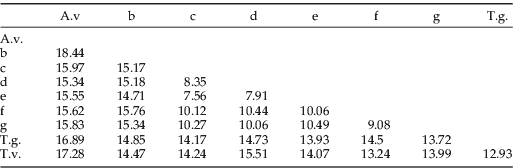
A.v., A. verbasci; T.g., T. granarium; T.v., T. variabile.
The values are nucleotide percentage differences (%).
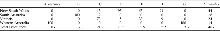
The distribution of each clade was visualised on a distribution map (fig. 2). The majority of specimens that were placed in clades d and f (95% and 91%, respectively) were mainly observed in the southern part of New South Wales, and 73% of clade c was found in Victoria (table 4). Clade b was only observed at Port Adelaide in South Australia, and clade g was only located at Varley in Western Australia. The specimens that clustered with the T. variabile reference specimens were found at 78% of the sites sampled (table 1).
Table 4. The distribution of each species per state.

Genetic structure of T. variabile using COI
Cytochrome oxidase I was the only gene to resolve divergence within the T. variabile clade (table 2), revealing nine unique haplotypes (table 5). Network analysis of these haplotypes, using the program TCS v1.21 (Clement et al., Reference Clement, Posada and Crandall2000), revealed one main haplotype (H4) with four direct descendents (H2, H3, H6 and H8). One haplotype (H5) was distantly related to H4 (missing multiple mutational steps), and three haplotypes (H1, H7 and H9) were not connected in the network because their divergence ranged outside the 95% parsimony limit imposed by the program (fig. 3c). With no connectivity between H1, H7 and H9 and the rest of the haplotypes, the relatedness between these haplotypes could not be determined. Haplotype 4 was found at all the western and eastern states collection sites (where we identified the presence of T. variabile; table 4), except for Willow Tree that had only H5. Tamworth and Swan Hill both contained additional haplotypes that showed no connectivity.

Fig. 3. Spatial distribution of the nine T. variabile haplotypes. (a) Spatial distribution of T. variabile within Western Australia. (b) Spatial distribution of T. variabile on the east coast of Australia. (c) TCS network of the nine haplotypes. (d) Haplotype colour key. (e) Sampling areas within Australia where the presence of T. variabile was confirmed.
Table 5. Number of T. variabile haplotypes and frequency of each haplotype per collection site for the mitochondrial markers Cytochrome oxidase 1 (CO1).

Discussion
This study aimed to investigate the population structure of T. variabile in Australia to determine what factors may have influenced the unsuccessful outcome of the eradication campaign. The results revealed seven deeply distinct clades in both the all gene Parsimony and ML trees, and in COI trees (figs 1 and 2e, respectively) with average pairwise divergence between clades of 18.5% (SE 2.27) and 17.5% (SE 1.87%) for COI and CYT b, respectively. These data, consistent at both nuclear and mitochondrial gene loci, strongly suggest that seven distinct species were collected, of which only 47% (71) were clustered with the T. variabile reference sample (table 2). Population analysis of those specimens identified as T. variabile revealed one main haplotype with several derived haplotypes and three unconnected haplotypes that may be separate incursions. Both misidentification of captured specimens and possible multiple incursions would have a strong negative effect on the success of the eradication campaign.
Of the 153 individuals that were genotyped, only 46.7% could be grouped with the specimens that were morphologically verified as T. variabile. Since the specimens were macerated to liberate the DNA, we cannot attempt to match genetic and morphological patterns. However, our data strongly suggests that divergent clades were not T. variabile, as large nucleotide percentage differences were observed between clades (tables 2 and 3), implying deep evolutionary divergence and presumptive reproductive isolation. The average inter- and intra-specific divergence for the COI locus in this study was 18.5% and 0.48%, respectively. In comparison, the inter- and intra-specific divergence levels for the COI loci, previously determined for a multitude of insect pests (Cognato, Reference Cognato2006), are an average of 7.4% (2–24%) and 1.75% (0.077–26%), respectively. The mean inter-clade divergence observed in our study was more than double this previous report, and the intra-clade divergence was only a fraction of that calculated by Cognato (Reference Cognato2006), which further supports the presence of a number of deeply divergent cryptic species in the present study. Furthermore, T. variabile and T. granarium, which can be differentiated using morphological keys, had a COI divergence of 18.8% (table 3), the lowest observed between T. variabile and any other clade. With further study, morphological characters may be resolved that discriminate between the other cryptic species discovered in this study, making field recognition and management more feasible.
The six putative species, accounting for 53% (n=82) of the individuals analysed, could be attributed to both high trapping yields and the difficulty encountered when identifying samples collected from a trapping program. The traps were placed outside of the grain facilities, possibly to increase the number of T. variabile collected (Campbell & Mullen, Reference Campbell and Mullen2004), but this also potentially increases the number of native Dermestids collected, since some natives have been shown to be attracted to the pheromone used in the traps (unpublished data). The number of specimens collected in each trap was likely to have exceeded a few hundred (unpublished data) making identification particularly difficult, especially when adopting a quick visual screening approach. Morphological distinction between T. variabile and other closely related Trogoderma requires dissection and careful microscopic examination of the genitalia (Szito, Reference Szito2007), not just the examination of external characteristics. Dissection and preparation of the genitalia for examination requires time and skill, and would be impractical to perform on the number of samples collected at each site. If the eradication campaign adopted a similar approach and only examined the external characters, the likelihood of misidentification would be high and potentially result in the management of a non-target species.
In the future, for Trogoderma species, we suggest that a non-destructive method, such as the recently developed ANDE (Castalanelli et al., Reference Castalanelli, Severtson, Brumley, Szito, Grimm, Munyard and Groth2010), be used. The availability of such a non-destructive DNA extraction technique when this study was commenced would have allowed us to revisit the samples and identify each specimen using morphological techniques post grouping them into genetic lineages. Two years after the initial Chelex extractions, additional DNA samples (from the same trapping program) were extracted using the non-destructive ANDE method. However, the extracted DNA was subsequently shown to be severely fragmented resulting in unsuccessful amplification. We believe that this was not the result of the ANDE extraction method, since the T. variabile reference specimens were also collected using sticky traps, but this time the adhesive was not removed. Rather, the unsuccessful amplification can be attributed to the use of harsh chemicals, such as hexane or limoene used to remove the specimens from the sticky traps (Szito, Reference Szito2007), combined with long-term storage in ethanol at room temperature. We also observed limited amplification with Chelex samples. Only minimal genetic analysis has been conducted on the native and international dermestids; so until these sequences are detected again, with accompanying whole specimens, the six new species identified in this work will remain putative.
The genetic data set generated in this study allowed us exploration into possible genetic structure within T. variabile. Although sample sizes were low, several interesting trends were observed based upon the distribution and relatedness of haplotypes (table 5, fig. 3). The main T. variabile haplotype (H4) was found at all eastern and western Australian sites where T. variabile was present, except for Willow Tree in NSW. The distance between each of these sites ranged from 9 to 3760 km; and, considering that T. variabile has a limited dispersal range based on its ecology (Campbell & Mullen, Reference Campbell and Mullen2004), human-aided transport is the plausible dispersal means. The three non-connected haplotypes observed at Tamworth (NSW) and Swan Hill (Vic) are interesting because they are localised and yet to disperse, suggesting that they are younger – such is the expectation based on coalescent theory (Kingman, Reference Kingman1982; Crandall & Templeton, Reference Crandall and Templeton1993). However, we are unable to ascertain if this is the result of multiple incursions or a single incursion that contained multiple haplotypes. Increased sampling within Australia and additional samples from international areas would be needed to confirm the multiple incursion events, and additional samples from international areas would be needed to confirm the multiple incursion events.
With increasing international trade, the likelihood of serious pests invading Australia will inevitably increase. When an invasive species is detected, the success of control or eradication is dependent on accurate identification (Walter, Reference Walter2003; Schutze et al., Reference Schutze, Mather and Clarke2006). This study revealed that 53% of the specimens collected during the 2001 to 2003 T. variabile trapping program were misidentified, and only 78% of the sites actually contained T. variabile. We believe this to be the result of dealing with several hundred samples per site, as well as the use of a quick screening method to identify T. variabile. Without keying out each specimen fully, misidentification is inevitable. Regardless of the method of morphologically based identification adopted in the eradication program, this study strongly implies that the presence of several cryptic species would have thwarted successful eradication or containment of the incursion. Misidentification would have seriously compromised the eradication campaign through the calculation of incorrect estimates of population size and location, with resulting in misdirection of resources (Walter, Reference Walter2003). Furthermore, analysis of T. variabile populations suggested large-scale movement aided by human dispersal (up to approx. 3750 km), but more concerning were the numerous haplotypes that were not derived from the main population. Australia's grain industry should be highly concerned that the Khapra beetle may be allowed to infiltrate our borders under the mistaken identity of T. variabile.
Acknowledgements
This work was supported by the CRC for National Plant Biosecurity and Australian Government by the 2007 Science and Innovation Awards for Young People in Agriculture, Fisheries and Forestry as awarded to K.M. Mikac. We would like to thank the two anonymous reviewers for their comments that improved the quality of the manuscript. Thanks to Jane Wright, CSIRO, for providing the specimens collected in CSIRO survey.