1. Introduction
Mud flows are natural hazards which can cause extensive damage, yet they are still very difficult to predict. At the surface of such destructive events, unstable waves can develop and sometimes reach very large amplitudes (up to  $3\ \mathrm {m}$ for the Yellow river in August 1977, as reported by Engelund & Zhaohui (Reference Engelund and Zhaohui1984), quoting Qian, Wan & Qian (Reference Qian, Wan and Qian1979)). These waves can travel much faster than the primary flow, and therefore can have very destructive power. They need to be taken into account in any risk assessment (Köhler et al. Reference Köhler, McElwaine, Sovilla, Ash and Brennan2016). Mud and slurries, when they flow down a slope, are usually described as visco-plastic fluids. This large family encompasses very different fluids involved, for example, in industry (hydrocarbons, concrete, cosmetics, biomedical materials, emulsions), in food processing (jam, butter, ketchup, mayonnaise) or in other natural phenomena (lava flows (Blake Reference Blake1990), avalanches (Nishimura & Maeno Reference Nishimura and Maeno1987), debris flows (Iverson Reference Iverson1997)). Those fluids have in common two characteristics: (i) they exhibit a yield-stress behaviour, i.e. they need to undergo a minimal stress to flow, otherwise they behave as a solid, and (ii) their viscosity decreases when the shear rate increases (shear-thinning). This rheological behaviour is often described by the Herschel–Bulkley model (Herschel & Bulkley Reference Herschel and Bulkley1926), with a constitutive law:
 \begin{equation} \left. \begin{array}{ll} \tau = \tau_{y}+K\dot{\gamma}^{n}, & \text{when } \tau>\tau_y,\\ \dot{\gamma} = 0, & \text{when } \tau<\tau_y, \end{array} \right\} \end{equation}
where  $\tau _y$ is the yield stress,
  $K$ the consistency index and
  $n$ the flow index (the case
  $n=1$ is called Bingham fluid (Bingham Reference Bingham1922)). Here,
  $\tau$ refers to the second invariant of the deviatoric stress tensor, and
  $\dot {\gamma }$, the shear rate, refers to the second invariant of the rate-of-strain tensor. It is known that an unperturbed film flow down a slope has a shear stress that grows linearly with depth from zero at the surface. When the fluid is visco-plastic, this has the consequence that there is a region close to the surface where the shear stress is smaller than the yield stress, leading to an apparent solid, unsheared region, with a uniform velocity, known as a plug flow. This characteristic first misled the theoreticians into believing that this system was similar to a Poiseuille flow of a visco-plastic fluid, with very high stability thresholds, significantly higher than for a Newtonian fluid (Frigaard, Howison & Sobey Reference Frigaard, Howison and Sobey1994). Yet, such high stability thresholds were in contradiction with observations in the experiments (Coussot Reference Coussot1994). This paradox was resolved by Balmforth & Craster (Reference Balmforth and Craster1999), who pointed out that the hypothesis of the plug region at the surface being a true elastic solid was incompatible with thickness variations in the flow, as observed, for example, at surge fronts or when flowing over an obstacle. They stated that the ‘plug’ region was in fact an approximation of order
  $0$ in
  $\epsilon$, the ratio between the typical thickness and the typical length of the film, assumed to be small. They proposed to introduce a new model, in which the flow speed is expressed as an asymptotic expansion in
  $\epsilon$. If, in this model, the term of order
  $0$ still exhibits a uniform velocity close to the surface, this is not the case of higher order terms of the expansion, which are found to be varying even close to the surface. In other words, the ‘plug’ region is in fact sheared, and the shear rate in this region is of order at least
  $O(\epsilon )$. This is possible even if the shear stress (i.e. the off-diagonal component of the deviatoric stress tensor) drops below the yield stress, because height variations induce longitudinal speed variations, which in turn induce a non-zero deviatoric stress along the flow, and in the end,
  $\tau$ the second invariant of the full deviatoric stress tensor remains larger than the yield stress
  $\tau _y$.
With this idea, they were able to study the roll-wave-like instability in muds. This instability has the same physical origin, i.e. inertia, as in Newtonian fluids (Smith Reference Smith1990) and in other non-Newtonian fluids (Millet et al. Reference Millet, Botton, Rousset and Ben Hadid2008). They calculated the linear stability threshold of a visco-plastic film flow with the Orr–Sommerfeld approach, considering the lowest order in  $\epsilon$ in the sheared region, and the first order in
  $\epsilon$ in the pseudo-plug region (Balmforth & Liu Reference Balmforth and Liu2004). From the obtained equations, they were able to perform a long-wave expansion, and to obtain a critical Reynolds number
  ${Re}_c^{Bal}$, above which infinitesimal long-wave perturbations are amplified:
 \begin{align} {Re}_c^{Bal}= \dfrac{[1+n+2nBi(1+nBi)](1+n)(2+n)(2+3n)(1-Bi)^{{-}2/n}}{2(2+n)(1+n)^{2}+n(2+n)(7+9n)Bi+(11+19n+6n^{2} )(2+nBi) n^{2} Bi^{2}} \end{align}
with  $n$ the flow index and
  $Bi$ the Bingham number defined as the ratio between yield stress and maximum viscous shear stress. In this model, the onset of instability depends only on
  $Bi$ and
  $n$. Here
  $Re_C^{Bal}$ diverges when
  $Bi \rightarrow 1$ because of the term
  $(1-Bi)^{-2/n}$, and this divergence is all the more strong as
  $n$ is small. This singular limit corresponds to the transition towards a full flow arrest, a situation which cannot then exhibit unstable roll-waves. It is important to note that even if the influence of the pseudo-plug, where the velocity gradient is of order 1 in
  $\epsilon$, is taken into account, only the 0th order terms are kept in the equations. In other words, the model is still of order 0 in
  $\epsilon$. For this reason, their model did not get unanimous support in the literature. In fact, Fernández-Nieto, Noble & Vila (Reference Fernández-Nieto, Noble and Vila2010) (F.N.) criticised the validity of a 0th order approach, and showed that an additional term of order
  $\epsilon$ should be accounted for to derive the expression of the critical Reynolds number, at least for a Bingham fluid. When translated in the formalism used by Balmforth & Liu (Reference Balmforth and Liu2004), they found an expression for a Bingham fluid:
 \begin{equation} {Re}_c^{F.N.} = \dfrac{5[1+Bi+Bi^{2} - 3 \epsilon ({\rm \pi} Bi^{2}/4) ] } {3Bi^{5} - 5Bi^{3} + 2} \end{equation}
which corresponds to (1.2) for  $n=1$ with an additional term of order
  $\epsilon$. Until now, based on the literature of experimental works on the subject, it has not been possible to validate any of these approaches. In fact, on the experimental side, the literature is not abundant. The first to experimentally visualise this sort of surface waves in Newtonian fluids was Kapitsa & Kapitsa (Reference Kapitsa and Kapitsa1949), but it was not before the 1990s that the critical Reynolds number of the roll-waves instability was measured by Liu, Paul & Gollub (Reference Liu, Paul and Gollub1993), again for a Newtonian fluid, confirming the theory of Benjamin and Yih (Benjamin Reference Benjamin1957; Yih Reference Yih1963). This work inspired other scientists to investigate the stability for non-Newtonian fluids, for example, Forterre & Pouliquen (Reference Forterre and Pouliquen2003) in the different, but related, context of granular flows or Allouche et al. (Reference Allouche, Botton, Millet, Henry, Dagois-Bohy, Güzel and Ben Hadid2017) for shear-thinning fluids. The latter showed that shear-thinning properties tend to destabilise the flow. More recently, Freydier, Chambon & Naaim (Reference Freydier, Chambon and Naaim2017) looked into the influence of terms of higher order in
  $\epsilon$, thanks to an original set-up of a stationary surge. However, they mainly focused on the front study, and did not look into the stability of the nearly uniform part of the flow. To our knowledge, very few experiments were performed on the stability of visco-plastic fluids down a slope (Coussot Reference Coussot1994; Tamburrino & Ihle Reference Tamburrino and Ihle2013). In particular, Coussot (Reference Coussot1994) was the first to investigate the presence of roll-waves in a rectangular channel. This seminal experimental work was, however, not designed to finely explore the stability under small controlled perturbations. In this paper, we experimentally investigate the primary instability of visco-plastic fluids down an inclined plane. In the next sections, we will describe the experimental set-up, the fluids used and the measurements made. Finally, we will compare our results with the theory of Balmforth & Liu (Reference Balmforth and Liu2004) for the stability thresholds, wave numbers and growth rates.
2. Experimental set-up
In this section, we describe the system we designed to produce film flows down an incline, with a clean and controlled surface perturbation, and indicate how to measure and characterise the stability of the waves produced this way. This set-up was originally the same as in Allouche et al. (Reference Allouche, Botton, Millet, Henry, Dagois-Bohy, Güzel and Ben Hadid2017), but had to be adapted to work with yield-stress fluids.
2.1. Flow and perturbation system
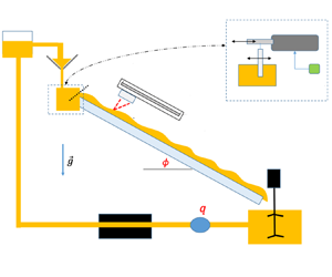
The set-up consists in a film flowing down a long channel ( $2\ \mathrm {m}\times 0.5\ \mathrm {m}$), as shown in figure 1(a,b): the fluid is collected at the channel output in a tank (collector), and sent back to the inlet by a volumetric pump (PCM EcoMoineau) through a manifold at the channel entrance, creating a permanent regime. The channel angle
  $\phi$ is adjustable between
  $0$ and
  $15 \pm 0.5$ degrees, and the flow rate is controlled by the volumetric pump, up to
  $1\ \mathrm {L}\,\mathrm {s}^{-1}$. Flow rate
  $q$ is also measured between the output tank and the pump using a Rosemount™ electromagnetic flow meter. A typical experiment requires roughly
  $70\ \mathrm {L}$ of fluid to work properly. Controlled perturbations are generated at the flow surface using a plate plunging into the collector at the entrance of the channel. This plate is connected to a shaker (B
 $\&$K 4809) vibrating in the flow direction, itself driven by a low frequency generator. The generator produces an electric sine wave of frequency
  $f$, converted by the shaker into a sinusoidal, quasi-plane wave also of frequency
  $f$, at the surface of the flow. The amplitude voltage is kept small enough so that the height of the surface perturbation remains sinusoidal close to the entrance channel, i.e. the initial perturbations are kept in the linear regime (note also that there is no need to amplify the electric signal between the generator and the shaker to produce and measure small perturbations). The flow must also be isolated from external (and undesired) perturbations, in particular from the pump. To mitigate these disturbances, we have placed two additional damping tanks with a free surface between the pump and the channel entrance, and we have taken great care to isolate the channel body from any other parts of the circuit connected to the pump, as well as from the ground (the set-up is placed on rubber wedges). In summary, a film flow is generated with a flow rate
  $q$, in a channel inclined at an angle
  $\phi$, and with a controlled sine perturbation of its thickness, at frequency
  $f$.
$f$.

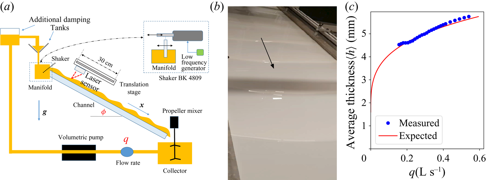
Figure 1. (a) Scheme of the experimental set-up. Here, g is the gravitational acceleration. (b) View of the experiment with unstable roll waves. Horizontal shadow is due to the measuring apparatus. (c) Average flow thickness: values measured (sensor) and curve expected from flow rate and measured rheology, with a uniform flow hypothesis.
2.2. Fluids
In our experiments, two types of visco-plastic fluids have been used: (i) carbopol and (ii) kaolin.
2.2.1. Carbopol microgel
Carbopol is a highly cross-linked polyacrylic polymer, which adopts the structure of a microgel at neutral pH (Ketz, Prud'homme & Graessley Reference Ketz, Prud'homme and Graessley1988). The concentration of microgel particles is directly related to the initial concentration of the polymer, so it is possible to tune the rheology of the fluid by changing the initial polymer concentration. Note that the flow index remains roughly constant. To prepare the fluid, we start by dissolving powder of carbopol (carbopol 980™ by Lubrizol) in a can filled with water while continuously stirring the mixture. After two hours, the polymer is dissolved and the solution is homogeneous. Then the fluid is left at rest for 2–3 days to get rid of air bubbles and finish the dissolution. After that, water is added to the solution to reach a desired weight fraction, usually between  $1.5\times 10^{-3}$ and
  $2 \times 10^{-3}$ for a total volume of
  $70\ \mathrm {L}$. The solution is then neutralised in pH by adding sodium hydroxide (
 $\mathrm {NaOH}$), giving the fluid its final visco-plastic behaviour. The choice of Carbopol 980 prepared with low stirring at these weak concentrations ensures that the fluid thixiotropic and visco-elastic properties can be neglected (Piau Reference Piau2007; Dinkgreve et al. Reference Dinkgreve, Fazilati, Denn and Bonn2018). Finally, to allow the film thickness to be measured using a triangulation position sensor (see § 2.3), the solution is made opaque by the addition of 50 g of titanium dioxide (
 $\mathrm {TiO}_2$).
2.2.2. Kaolin slurry
The second fluid is obtained by mixing approximately  $40\ \mathrm {kg}$ of kaolin powder with 35–45 kg of water, resulting in a visco-plastic fluid of density
  $d\simeq 1450\ \mathrm {kg}\,\mathrm {m}^{-3}$. The fluid is constantly mixed in the collector tank throughout the experiments to avoid sedimentation. Two kaolin powders have been used, one from Hostun quarry (near Grenoble, France) and the other from Quessoy quarry (near St-Brieuc, France). Only batches with similar rheological properties, in particular the flow index
  $n$, have been kept. Given the experimental conditions (permanent regime, permanent shear rate), we assume that the visco-plastic behaviour is dominant compared with any other effects (specially visco-elasticity and thixiotropy), similarly to Chambon, Ghemmour & Laigle (Reference Chambon, Ghemmour and Laigle2009). Moreover, flow rates in the experiments are always small enough to ensure a regular visco-plastic behaviour (Coussot Reference Coussot1995).
2.2.3. Rheological characterisation
During the experiments, fluid samples are regularly taken for characterisation. The rheology of the fluids under study is measured with a cone-plate rheometer (Lamy Rheology Instrument Rheometer RM 200 Touch), with rough surfaces to avoid slippage at low shear rates (Coussot & Piau Reference Coussot and Piau1994; Piau Reference Piau2007). The measurement consists in rotating the top plate at different imposed rotating speeds and measuring the torque, with both quantities converted into shear rate and stress, in ramp-up then ramp-down series. To measure steady-state values, the measurement duration is adapted to the rotating speed (the faster the rotation, the shorter the measurement). The flow curves obtained always follow the Herschel–Bulkley law (see (1.1) and figure 2(a) for a typical curve). By varying the concentration in carbopol or kaolin, we are able to obtain fluids with rheological parameters within the ranges given in table 1. Homogeneity of the fluid is verified by comparing the rheology of samples taken at various places of the set-up. We observe also a slow variation of the rheological properties in time, due to different effects depending on the fluid: water evaporation for kaolin and acidification by  $\mathrm {CO}_2$ dissolution for carbopol (see figure 2b,c). Rheological properties are checked at regular intervals throughout the experiments (every one to three hours), in order to determine time windows over which we can consider that the fluid being studied does not change. As illustrated in figure 2, the typical yield-stress variation with time is over 2 weeks, whereas a series of experiments has never lasted more than one day. In fact, the slow variation of the yield stress over time has been our most reliable way of finely tuning the rheology of the fluids.
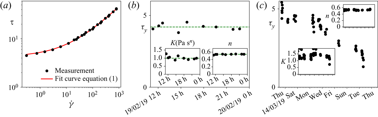
Figure 2. (a) Herschel–Bulkley fit of a typical experimental flow curve for carbopol, with fitted parameters  $\tau _y = 4.2\ \mathrm {Pa}$,
  $K = 0.99\ \mathrm {Pa}\,\mathrm {s}^{n}$,
  $n = 0.54$. (b) Evolution of rheological parameters over a typical experiment series with carbopol. Green lines correspond to median values. (c) Evolution of rheological parameters over different series of experiments with carbopol. The yield stress slowly decays with time, probably due to water acidification.
Table 1. Ranges of the measured rheological parameters.

2.3. Local thickness measurement
Film thickness is measured with a laser triangulation sensor (Micro-Epsilon optoNCDT 1420) as illustrated in figure 1. A laser is shot at the film surface, a spot appears on the surface by light diffusion, and the distance from this spot to the sensor is measured using triangulation. This allows us to measure the thickness over a region less than  $0.5\ \mathrm {mm}$ wide, and with a theoretical precision of
  $1\ \mathrm {\mu }\mathrm {m}$, small enough to detect perturbations of a few
  $10\ \mathrm {\mu }\mathrm {m}$. However, we have been surprised to measure a constant offset of a few
  $100\ \mathrm {\mu }\mathrm {m}$ for a given experiment series, between the spatio-temporal average of the measured thickness, noted
  $\langle h\rangle$ (see below), and the thickness expected from the rheology, assuming a uniform flow (see figure 1c). We believe this is due to the strong optical penetration of both fluids used, stronger than for typical opaque solid surfaces. Even if this offset did not affect the wave measurements (growth rates and wavelengths), we have decided to exclude every series with a difference between measured and predicted thicknesses greater than 10 %, and otherwise to correct the measured thickness with the offset. The sensor is fixed to a linear translation stage (Zaber LSQ300-B) able to move along the flow over
  $30\ \mathrm {cm}$ with a speed of
  $1\ \mathrm {cm}\,\mathrm {s}^{-1}$. If we assume the film is perturbed by a linear plane sine wave of the form
  $h(x,t) = \langle h\rangle + h_0 \textrm {e}^{ \alpha x} \cos ( 2{\rm \pi} f t-kx)$, with
  $\alpha$ the spatial growth rate,
  $k$ the wavenumber, and
  $h_{0}$ the wave amplitude, the signal
  $h_s$ measured by the sensor over a translation at speed
  $v$ (see a typical signal in figure 3a) takes the following form:
 \begin{equation} h_{s}(t) = \langle h\rangle + h_0 \textrm{e}^{\alpha v t} \cos (2{\rm \pi} f t - kvt). \end{equation}
To extract the spatial growth rate  $\alpha$ and wavenumber
  $k$, the Fourier transform of the signal is analysed following Yoshida et al. (Reference Yoshida, Sugai, Tani, Motegi, Minamida and Hayakawa1981). Close to the imposed frequency of the perturbation, the form of the discrete Fourier transform
  $\mathcal {F}$ of the real signal
  $h_s$ shows a peak, and can be approximated in its vicinity as
 \begin{equation} \mathcal{F}[h_s](\,f_m)= \dfrac{A}{f^{{\star}}-f_m}+B+Cf_m, \end{equation}
with  $\,f^{\star } = (\,f-kv/2{\rm \pi} )-\textrm {i} \alpha v/2{\rm \pi}$ the complex frequency,
  $\,f_m$ the
  $m{\text {th}}$ Fourier frequency,
  $A$ a prefactor that includes amplitude and sampling rate,
  $B$ a constant (white noise) and
  $C f_m$ a linear variation in spectrum, which approximates any other resonances far from
  $f$. By taking the ratio of finite differences of the Fourier transform close to the resonance peak, it is possible to eliminate the unknown constants
  $A$,
$A$,  $B$ and
  $C$, in order to extract directly the value of
  $\,f^{\star }$, which then simply yields
 \begin{equation} k = 2{\rm \pi}\dfrac{f-\mathrm{Re}(\,f^{{\star}})}{v}\quad \textrm{and}\quad \alpha ={-}2{\rm \pi} \dfrac{ \mathrm{Im} (\,f^{{\star}})}{v}, \end{equation}
where  $\mathrm {Re}(\,f^{\star })$ and
  $\mathrm {Im}(\,f^{\star })$ refer to the real and imaginary parts of the complex number
  $\,f^{\star }$. See an example of a real signal and its Fourier transform in figure 3.
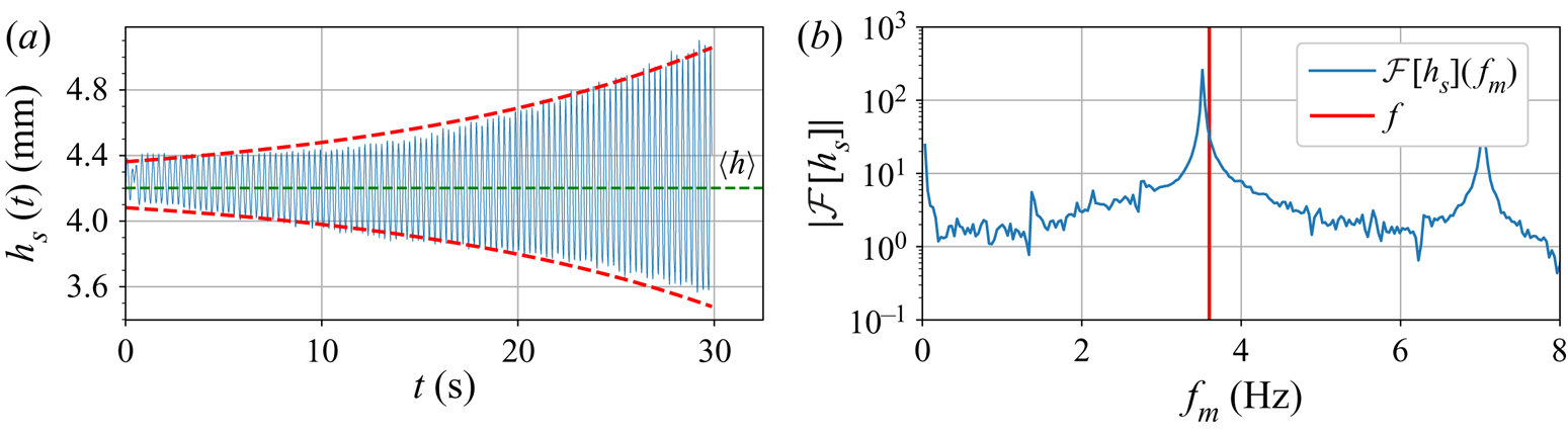
Figure 3. (a) Blue: typical measured signal  $h_s(t)$. Red: signal envelope
  $h_0\textrm {e}^{\alpha vt}$, with
  $\alpha$ given by (2.3a,b). (b) Blue: Fourier transform of signal
  $h_s(t)$. Red: imposed frequency at
  $3.6\ \mathrm {Hz}$. The main peak is at a frequency
  $\mathrm {Re}(\,f^{\star }) = f - kv/2{\rm \pi}$, slightly shifted from the imposed frequency.
3. Linear stability measurement
In this section, we explain how we determined the stability map from our measurements. The determination of the linear stability thresholds consisted of the following steps. First, we fixed the frequency  $f$, the flow rate
  $q$ and the angle of inclination
  $\phi$, and we measured the spatial growth rate
  $\alpha$ and the wavenumber
  $k$. We then repeated the measurement at different frequencies. Figure 4(a) shows the variation of the typical growth rate
  $\alpha$ with
  $f$ for a given flow rate. The cutoff frequency
  $\,f_c$ is deduced as the frequency above which the flow is stable (
 $\alpha <0$). At very low frequencies (
 $\,f<0.5\ \mathrm {Hz}$), the measured growth rates are not reliable because the shaker transfer function decays rapidly when
  $\,f\rightarrow 0$. We repeated the process at different flow rates (slope fixed), to obtain the evolution of
  $\,f_c$ with
  $q$. Figure 4(b) shows the stability diagram in the
  $(q,f)$ plane. We identified the unstable regime (
 $\,f< f_c$) and the stable regime (
 $\,f>f_c$). We also can see that under a critical flow rate, the flow is always stable. To summarise and discuss these results, we need to convert the critical flow rate into critical Reynolds and Bingham numbers. As in Balmforth & Liu (Reference Balmforth and Liu2004), we can regroup the parameters on which depends the flow in four dimensionless groups, which we chose to be
  $n, \phi , {Re}, Bi$. For the last two groups, we adopted the Balmforth & Liu (Reference Balmforth and Liu2004) conventions
 \begin{equation} {Re}= \dfrac{\rho\tan(\phi)}{K} \left( \dfrac{\rho g \langle h\rangle^{1+n} \sin \phi}{K} \right)^{({2-n})/{n}} \langle h\rangle^{n}\quad \text{and} \quad Bi=\dfrac{\tau_{y} }{ \rho g \langle h\rangle \sin \phi}. \end{equation}
The Bingham number  $Bi$ compares the yield stress of the fluid to the maximum shear stress in the flow, and the Reynolds number
  $Re$ is based on a typical flow speed
  $V= (\rho g \langle h\rangle ^{1+n} \sin \phi /K )^{1/n}$ and a typical viscosity
  $\mu =K (V/\langle h\rangle )^{n-1}$. In the results presented hereafter for the thresholds, we will see that for the rather low values of the angle
  $\phi$ used in the experiments, the stability threshold does not depend on
  $\phi$, apart from its influence through
  $Re$ and
  $Bi$ (3.1a,b). As a consequence, our objective was to measure a stability boundary in the form
  ${Re}_c = f(Bi, n)$. Unfortunately, in our experiments, when
  $\phi$ and rheology are fixed,
  ${Re}$ and
  $Bi$ both vary with the dimensional parameter
  $q$ and it is not possible to work with
  $Bi$ kept constant. This led us to define both a critical Reynolds number
  ${Re}_c$ and a critical Bingham number
  $Bi_c$ at the extremity of the marginal curve (
 $\,f\rightarrow 0$), and to compare them to the theory. Figure 5 shows the stability diagram of figure 4(b) translated in the planes
  $(Re,f)$ and
  $(Bi,f)$, with the critical Reynolds and critical Bingham numbers determined with a square root fit of the marginal curve, following the Liu et al. (Reference Liu, Paul and Gollub1993) approach. In order to compare the results to the Balmforth & Liu (Reference Balmforth and Liu2004) prediction, we repeated this measurement at different
  $\phi$ and for different rheologies (
 $\tau _y$ and
  $K$), to explore the
  $(Re,Bi)$ plane, but with the same fluid type to keep
  $n$ roughly constant. Finally, figure 6 shows the critical Reynolds and critical Bingham numbers for two different
  $n$, corresponding to the two different fluids.
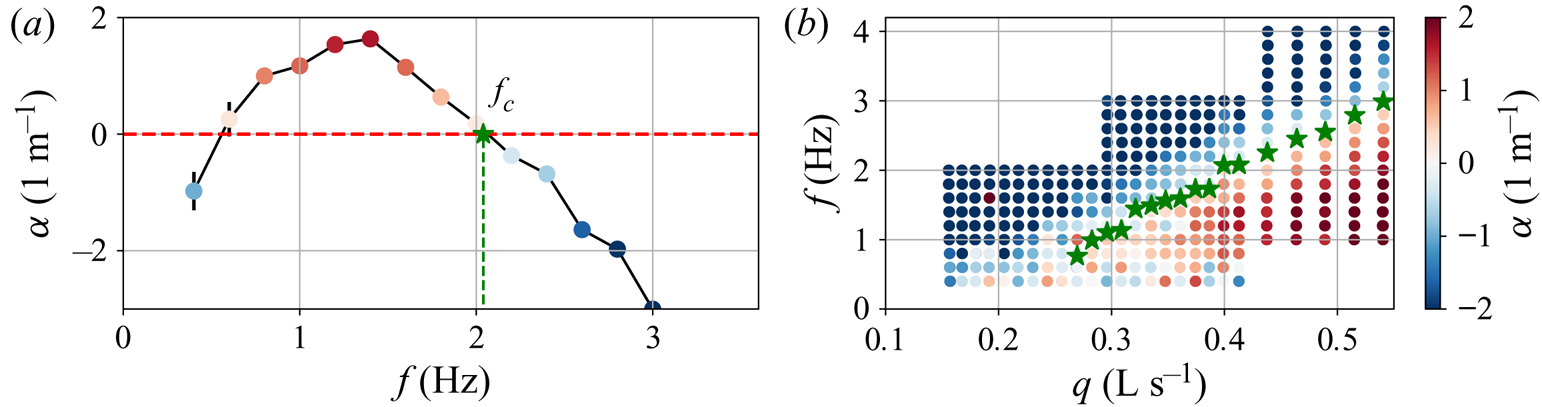
Figure 4. (a) Variation of the growth rate  $\alpha$ with the frequency
  $f$, at flow rate
  $q=0.412\ \mathrm {dm}^{3}\,\mathrm {s}^{-1}$ and at angle
  $\phi = 15.6^{\circ }$, for carbopol with a rheology
  $\tau _{y}=4.21\ \mathrm {Pa}$,
  $K=0.99\ \mathrm {Pa}\,\mathrm {s}^{n}$,
  $n=0.54$. (b) Stability map in the
  $(q, f)$ plane (same
  $\phi$ and rheology as in panel a). Green stars: cutoff frequencies. In both pictures, colours correspond to growth rate
  $\alpha$ (see the scale in panel b).
Figure 5. Stability maps in the planes  $(Re,f)$ (a) and
  $(Bi, f)$ (b). Green stars: experimental cutoff frequencies. Red curves: square root fit. Red squares: critical Reynolds (a) and Bingham (b) numbers. Colours: growth rate. The fluid under study is the same as in figure 4.

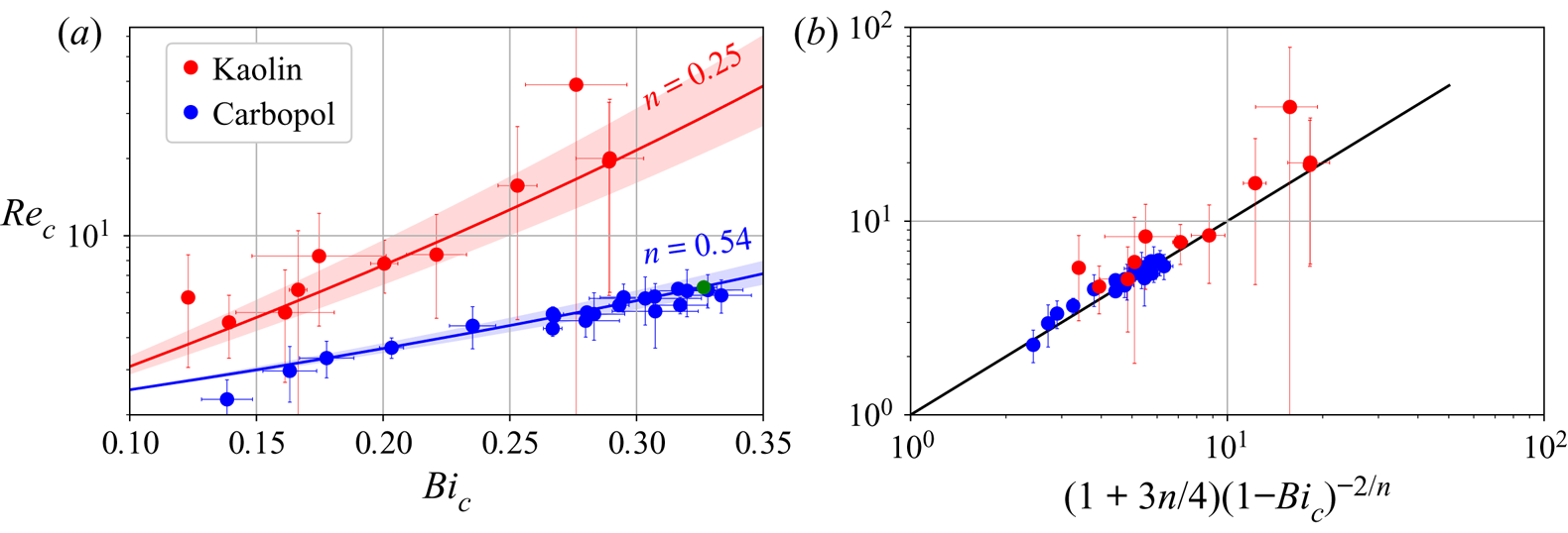
Figure 6. (a) Variation of  ${Re}_c$ with
  $Bi_c$, for the two fluids. Large error bars are due to
  $Re_c$ fit results falling outside of the measurement range. Solid lines: predictions from Balmforth & Liu (Reference Balmforth and Liu2004) (1.2). Shaded areas: same predictions for ranges of
  $n$ given in table 1. Green circle: case studied in figures 4 and 5. (b) Variation of
  ${Re}_c$ as a function of
  $(1+3n/4)(1-Bi_c)^{-2/n}$. Black solid line: identity.
4. Results and discussion
Figure 6(a) shows the variation of the critical Reynolds number with the critical Bingham number. Because the dimensionless numbers depend strongly on  $n$, using two fluids allowed us to span almost two decades in
  ${Re}_c$. Over this range, the experimental thresholds seem very well captured by the model of Balmforth & Liu (Reference Balmforth and Liu2004), even for the kaolin slurry (
 $n=0.25$), for which the experimental error was important. We observe also that
  ${Re}_c$ increases with
  $Bi_c$, which is consistent with the stabilising effect that we expect if
  $\tau _y$ increases or if
  $\phi$ decreases, since
  $Bi_c$ increases in both cases. In fact, this corresponds to a divergence of
  ${Re}_c$ when
  $Bi_c\rightarrow 1$, as predicted by Balmforth & Liu (Reference Balmforth and Liu2004). This explains why we could not see any unstable perturbation for
  $Bi>0.35$ in our set-up. A reasonable simplification of the
  ${Re}_c(Bi_c)$ relation can be obtained from (1.2) if we approximate the polynomial fraction, in factor of the diverging term, by the average of its extreme values in the interval
  $Bi \in [0, 1]$:
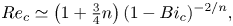 \begin{equation} Re_c \simeq \left(1+\tfrac{3}{4}n\right)(1-Bi_c)^{{-}2/n}, \end{equation}
as we can see in figure 6(b).
To discuss further these results, we would like here to recall how the threshold prediction by Balmforth & Liu (Reference Balmforth and Liu2004) was obtained. They solved the linear stability problem through an Orr–Sommerfeld approach, for a Herschel–Bulkley fluid, with the following features in particular:
(i) the film thickness is small enough to neglect any term of order 1 or more in
 $\epsilon$, the aspect ratio of the film defined as thickness over length ($\epsilon$ is chosen as $\tan \phi$ for convenience by Balmforth & Liu (Reference Balmforth and Liu2004));
(ii) the dimensionless numbers
$Bi$ and $n$ are fixed;(iii) they perform a long-wave development in their temporal stability analysis of the form
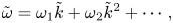
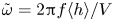
(4.2)with\begin{equation} \tilde{\omega} = \omega_1 \tilde{k} + \omega_2 \tilde{k}^{2} + \cdots, \end{equation}$\tilde {k} = k\langle h\rangle$ and $\tilde {\omega } = 2{\rm \pi} f \langle h\rangle / V$, the rescaled wavenumber and pulsation; and(iv) they define
${Re}_c$ as the ${Re}$ value that cancels the quadratic term $\omega _2$ in the development.


Surprisingly, a 0th order model in  $\epsilon$ seems sufficient to quantitatively predict the linear stability threshold, contrary to the claim of Fernández-Nieto et al. (Reference Fernández-Nieto, Noble and Vila2010). This does not mean that Fernández-Nieto et al. (Reference Fernández-Nieto, Noble and Vila2010) were wrong. In fact, their definition of Reynolds number, slightly different, makes the inertial terms appear in the equations as terms of order
  $\epsilon$. This definition could be convenient for cases where
  ${Re}$ in our definition and
  $\epsilon$ are of the same order of magnitude. In our experiments, we are not in this regime since
  ${Re}$ varies between 2 and 50, whereas
  $\epsilon =\tan \phi$ is at most
  $0.28$. Considering the prediction of Fernández-Nieto et al. (Reference Fernández-Nieto, Noble and Vila2010) for a Bingham fluid (1.3), we expect that the correction of order
  $\epsilon$ becomes more and more important when
  $Bi\rightarrow 1$. We also expect the prediction of Balmforth & Liu (Reference Balmforth and Liu2004) to be less accurate at larger angles, more likely because the choice of
  $\epsilon = \tan \phi$, i.e. the choice of a horizontal typical length
 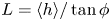 $L = \langle h\rangle / \tan \phi$, may not be relevant any more. Again, we were not able to reach those regimes in the experiments.
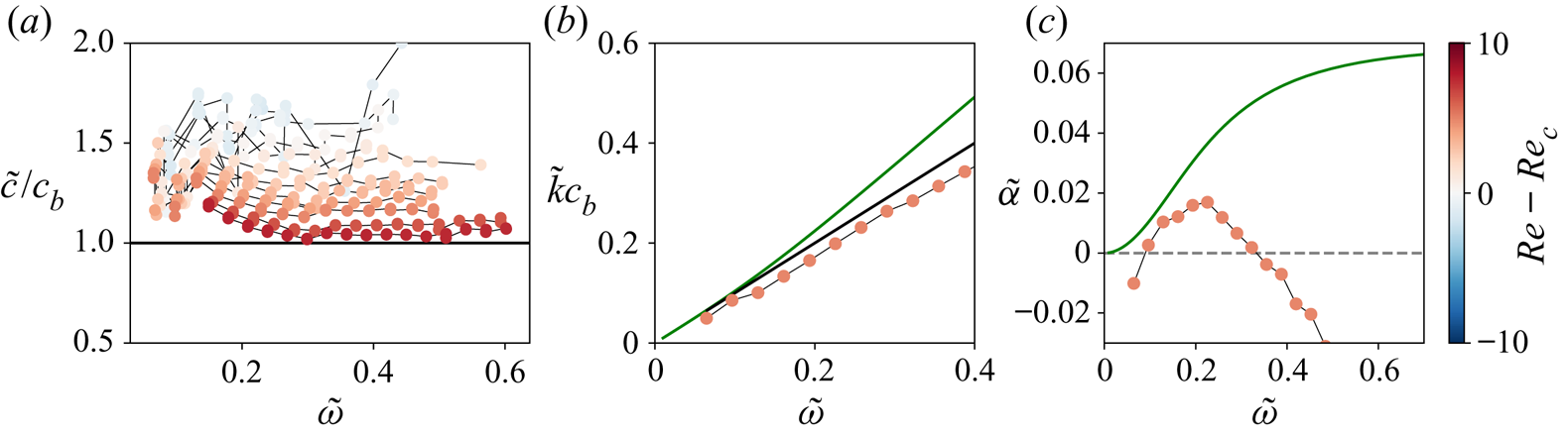
We will now look at the rescaled wavenumbers and dispersion relations, comparing our experiments with the model of Balmforth & Liu (Reference Balmforth and Liu2004) and their long-wave expansion (4.2). The first term calculated by Balmforth & Liu (Reference Balmforth and Liu2004) is found to be  $\omega _1 = (1-Bi)^{1/n}$. This suggests that the rescaled phase speed
  $\tilde {c}=\tilde {\omega }/ \tilde {k}$ should be constant at long waves and equal to
  $c_b = (1-Bi)^{1/n}$. At higher frequencies, the dispersion relation becomes nonlinear, when terms of order 3 in
  $\tilde {k}$ start to play a role. Moreover, this nonlinearity depends on the Reynolds number as well. In the experiments, where we perform spatial stability analysis, we expect to see similar effects: a constant phase speed
  $\tilde {c}$ equal to
  $c_b$ for long waves (low frequency) and nonlinear dispersion at higher frequencies. Figure 7(a) shows the normalised phase speed
  $\tilde {c}/c_b$ as a function of the rescaled pulsation
  $\tilde {\omega }$ for different
  ${Re}$. We observe that at a given
  ${Re}$, the phase speed
  $\tilde {c}$ reaches a plateau, and as
  ${Re}$ increases, the plateau gets closer to
  $c_b$. If part of this feature can be understood as an effect of the rescaling, as the rescaled pulsation
  $2{\rm \pi} f\langle h\rangle /V$ decreases with
  ${Re}$, it seems also that the long-wave approximation is all the more valid as
  ${Re}$ increases. We have numerically solved the model of Balmforth & Liu (Reference Balmforth and Liu2004) to compare it with the linear behaviour and our experiments. A typical example is shown in figure 7(b). We see that the wavenumbers predicted by Balmforth & Liu (Reference Balmforth and Liu2004) are systematically higher than those we measured, and that the deviation from the long-wave regime is more pronounced than in the experiments and occurs in the opposite direction. Moreover, when we compare the growth rates (see figure 7c), we observe that the model of Balmforth & Liu (Reference Balmforth and Liu2004) is also unable to predict the cutoff frequencies observed in the experiments. This is clearly a limit of dropping terms of order
  $\epsilon$ and higher order in the model. Indeed, those terms appear with powers of
  $\tilde {k}$ in the equations (see for example (3.3) in Balmforth & Liu (Reference Balmforth and Liu2004), at the order 2 in
  $\epsilon$). And such terms in
  $\epsilon \tilde {k}, \epsilon ^{2} \tilde {k}^{2},\ldots$ cannot be neglected when
  $\tilde {k}$ is of order
  $1/\epsilon$, i.e. at higher frequencies, and they have overall a stabilising effect on the waves. The comment of Fernández-Nieto et al. (Reference Fernández-Nieto, Noble and Vila2010) is then justified when it comes to predicting the wavelengths and growth rates: a model with higher order terms in
  $\epsilon$ is needed to describe properly wave dispersion mechanisms. Moreover, additional physical ingredients may be missing in the model to give a finer description of the dispersion effects, in particular visco-elasticity and surface tension effects.

Figure 7. For carbopol ( $n=0.54$), variation with the pulsation
  $\tilde {\omega }$ of (a) the normalised experimental phase speed
  $\tilde {c}/c_b$, at different
  ${Re}$, (b) the wave number
  $\tilde {k}$ times
  $c_b$ (dispersion relation), (c) the growth rate
  $\tilde {\alpha }$. Panels (b,c) correspond to the same case as in figure 4(a) (
 ${Re}=11.2$,
  $Bi=0.29$). Balmforth & Liu (Reference Balmforth and Liu2004) prediction, green line; for long waves, black line; experimental results, coloured circles.
5. Conclusion and perspectives
We described a series of experiments on visco-plastic film flows down an inclined plane. With a controlled perturbation set-up and an original wave characteristic measurement technique, we determined the stability map in the  $(Re, Bi)$ plane for two different fluids, with two different flow indices
  $n$. We have shown that the waves were weakly dispersive, at least in the explored range of frequencies. As we mentioned in the introduction,
  $\epsilon$, the aspect ratio of the film, is a key feature in existing prediction models. As such, it is crucial to know the highest order in
  $\epsilon$ needed to accurately describe the stability and the characteristics of the waves. Our experiments can provide a partial answer to this unsettled question: in the considered regimes, including terms of order
  $1$ or higher in
  $\epsilon$ appears not to be required to describe stability thresholds in terms of critical Bingham and Reynolds numbers. On the contrary, dispersion mechanisms are not well described by a linear model of order
  $0$ in
  $\epsilon$.
Acknowledgements
We thank G. Chambon and F. Rousset for fruitful discussions, E. Mignot for  $TiO_2$ supply, and S. Martinez and G. Geniquet for their help building the experimental set-up.
Declaration of interests
The authors report no conflict of interest.