II. Copula-Function Modeling

Copula functions originate from the work of Sklar (Reference Sklar1959), who developed a theorem stating that if F is a joint distribution function of m random variables (y ₁ ,…,y_m ) with marginal distributions F ₁ ,……,F_m , then there exists an m-dimensional copula C:[0,1] ^m  → [0,1] (from the unit m-cube to the unit interval) that satisfies the following three conditions:

1. 1. If the realizations of m-1 variables are known, each with a probability of 1, then the joint probability of the m outcomes is the same as the probability of the remaining uncertain outcomes a _n :

   (1) $$C\left( {1,\ldots,1,a_n, 1,\ldots,1} \right) = a_n \; {\rm for \; every}\,n \le m\,{\hbox{ and for all}}\,a_n \; {\rm in} \left[ {0,1} \right].$$

2. 2. The joint probability of all outcomes is zero if the marginal probability of any outcome is zero:

   (2) $$C\left( {a_1,\ldots, a_m} \right) = 0 \; {\rm if}\,a_n = 0 \; {\rm for \; any}\,n \le m.$$

3. 3. C is m-increasing, and the C-volume of any m-dimensional interval is non-negative.

Given F (y ₁ ,…, y _m ) with univariate marginal distributions F ₁(y ₁),…, F _m (y _m ) and inverse functions F ₁ ⁻¹,…, F _m ⁻¹, then

(3) $$y_1 \; = F_1 ^{ - 1} \left( {u_1} \right) \sim F_1,\ldots, y_m \; = F_m ^{ - 1} \left( {u_m} \right) \sim F_m, $$

where U = u ₁,…, u _m are uniformly distributed variates and

(4) $$ \eqalign{F\left( {y_1,\ldots, y_m} \right) &= F\left( {F_1 ^{ - 1} \left( {u_1} \right),\ldots,F_m ^{ - 1} \left( {u_m} \right)} \right) = {\rm Pr} \left[ {U_1 \le u_1,\ldots, U_m \le u_m} \right] \cr &= C\left( {u_1,\ldots, u_m} \right).}$$

C is the unique copula function associated with the distribution function and

(5) $$(F_1 \left( {y_1} \right),\ldots,F_m \left( {y_m} \right)) \sim C.^{} $$

If U ~ C, then

(6) $$\left( {F_1 ^{ - 1} \left( {u_1} \right),\ldots,F_m ^{ - 1} \left( {u_m} \right)} \right) \sim F.$$

Sklar's theorem demonstrates that any multivariate distribution can be written in terms of its univariate marginal distribution functions, along with a copula function that describes the dependence structure between the variables. The copula is a multivariate probability distribution for which the marginal probability distribution of each variable is uniform. A key element of Sklar's theorem is that in modeling a multivariate distribution, it allows for the separation in the modeling of the individual univariate marginal distributions from the dependence structure, captured by the copula function C. In particular, for an m-variate function F, the copula associated with F is a distribution function:

(7) $$C: \left[ {0,1} \right]^m \; \to \left[ {0,1} \right]{\rm that \; satisfies}\,F\left( {y_1,\ldots, y_m} \right) = C(F_1 \left( {y_1} \right),\ldots,F_m \left( {y_m} \right);\theta ),$$

where θ is a vector of parameters referred to as the dependence parameter, measuring the dependence between the marginal distributions. In bivariate applications, θ is typically a scalar.

Goodness-of-fit testing for copula functions remains a complex and relatively unresolved area. Issues arise primarily due to the high dimensionality of the problem, particularly for copula modeling where m ≥ 3. Summaries of the problems and approaches attempted in terms of copula goodness-of-fit testing are provided by Fermanian (Reference Fermanian, Jaworski, Durante and Härdle2013), Okhrin (Reference Okhrin2012), Genest, Remillard, and Beaudoin (Reference Genest, Remillard and Beaudoin2009), and Berg (Reference Berg2009), among others. In general, the power of the tests proposed to date differs depending on the sample size, the dimensionality, and the copula function being tested (Berg, Reference Berg2009). Although there is no universally agreed-upon methodology, a practical and frequently employed approach to bivariate copula selection is to use maximum-likelihood goodness-of-fit tests, such as the Akaike information criterion (AIC), to choose between copulas (Hasebe, Reference Hasebe2013).

Although the number of copula functions is theoretically infinite, parametric copulas can capture typical dependence structures between covariates, with known parameters that can be estimated. These parametric forms then allow the classification of copula functions into families. A description of copula families is provided in Nelsen (Reference Nelsen2006); two important examples worth noting are the elliptical and the Archimedean families. Copulas from the elliptical family include the Gaussian (normal) copula and the Student T copula. Although they do not have simple closed-form solutions, they are easily extendable to multivariate applications where m ≥ 3. However, they are limited to radial symmetry, restricting their ability to fully capture nonlinear, and particularly asymmetric, tail-dependence structures. Figure 1 provides simulation plots with 10,000 observations of typical Gaussian and T copulas.

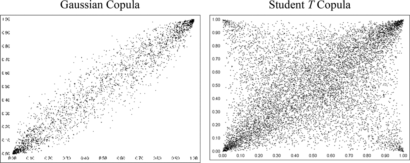
Figure 1 Bivariate Plots of Gaussian and Student T Copulas

Where different upper- and lower-tail behavior is called for, copulas from the Archimedean family may be employed. They include some relatively simple closed forms with dependence parameters that allow for asymmetric tail-dependence structures between covariates in a tractable way. In particular, upper- (λ _U ) and lower- (λ _L ) tail-dependence measures can frequently be derived from the copula parameters as well as, in limited cases, the relationship to standard dependence measures, such as Kendall's tau (τ_K) and Spearman's rho (ρ_S) (Cherubini, Luciano, and Vecchiato, Reference Cherubini, Luciano and Vecchiato2004).

Common forms of the Archimedean family employed are the Clayton, Gumbel, and Frank copulas. The Clayton copula allows for greater correlation, or tail dependence, in the lower values of the covariates, while the Gumbel copula captures tail dependency primarily in the higher values. The Frank copula captures greater correlation in the middle of the marginal distribution values as opposed to the tails. Figure 2 provides simulation plots of typical bivariate Clayton, Gumbel, and Frank copula functions generated with 10,000 observations. As can be observed in Figure 2, the Gumbel copula does capture some lower-tail dependence as well. The greater dependence in the middle of the marginal distributions, exhibited by the Frank copula, can be readily seen when compared to the plot of the Gaussian copula.

Figure 2 Bivariate Plots for Clayton, Gumbel, and Frank Copulas

It should be noted that through linear inversion (1 – a) of either, or both, of the two uniform distributions (a _n ), other forms of asymmetric tail dependence may be captured. Figure 3, for example, provides plots of the Clayton copula where a negative transformation of the x (a ₁ ) (Clayton (2)) or the y (a ₂ ) (Clayton (3)) covariate, or both (Clayton (4)), has been applied. Hence, asymmetric positive tail dependence can also be modeled employing the Clayton copula on the linearly inverted uniform variates.

Figure 3 Plots of Clayton Copula with Negative Transformation of Covariates

The relationship of the above-noted Archimedean copulas to their respective copula parameter θ, upper (λ _U ϵ [0,1]) and lower (λ _L ϵ [0,1]) asymptotic tail-dependence measures, and rank correlation measures, such as Kendall's tau and Spearman's rho, where tractable, is provided in Table 1, below.

Table 1 Archimedean Copulas and Dependence Parameters

In the case of the Frank copula, Kendall's tau and Spearman's rho require the calculation of the Debye function, where

$D_k \left( \alpha \right) = \displaystyle{k \over {\alpha ^k}} \mathop \int \limits_0^\alpha \displaystyle{{t^k} \over {\exp \left( t \right) - 1}}dt,\; \; \; k = 1,2$ .

The parameter of asymptotic upper-tail dependence, λ _U , is the conditional probability in the limit that one variable takes a very high value, given a high value in the other variable. Similarly, the asymptotic lower-tail dependence, λ _L , is the conditional probability in the limit that one variable takes a very low value, given a very low value in the other (Nelsen, Reference Nelsen2006).

In the case of the Clayton copula, an upper-tail-dependence measure results in a value of zero, as it is implicitly not measured. Similarly, the Gumbel copula parameter results in a lower-tail-dependence measure of zero. However, in both cases, as noted, linear inversions of the x and y covariates can result in implicit measures of upper- or lower-tail dependency, respectively. The Frank copula, which explicitly models dependency in the middle of the marginal distributions, results in upper- and lower-tail dependency values of zero.

III. Data and Analysis

We estimate and test the bivariate influence of Parker's scores on en primeur prices using a novel dataset obtained from http://www.bordoverview.com, created and maintained by the Dutch wine sellers Bolomey Wijnimport. The dataset comprises annual initial-release en primeur prices along with a number of wine critics’ barrel ratings, including those of Parker. It has been suggested that Parker's barrel ratings have had a significant impact on rising en primeur prices; therefore, we examine the period of 2004 through 2010, because this span includes the renowned 2005 harvest and a stable, sustained bull run in futures prices through 2010. Primarily due to the global economic recession, between 2010 and 2014, lower sales plagued the market and exerted downward pressure on prices. In addition, in 2003, Parker's barrel ratings were released after the en primeur prices were set by châteaux (Ali et al., Reference Ali, Lecocq and Visser2010).

A. Copula-Function Identification

Vose's ModelRisk software was employed to estimate various standard copula functions in defining the bivariate relationship between prices and Parker's ratings. In particular, the nonlinear relationship was examined for each year in the sample to determine the stationarity of the bivariate relationship, as well as for each Left and Right Bank vintage. As noted above, the issues surrounding goodness-of-fit tests arise primarily due to the high dimensionality of the problem (Fermanian, Reference Fermanian, Jaworski, Durante and Härdle2013; Panchenco, Reference Panchenko2005). However, a standard approach to copula-function modeling is to fit several copula functions to the data and apply maximum-likelihood goodness-of-fit tests to identify which functional form models the dependency structure relatively better. This approach does not provide for a power of the test, and complexities still exist with respect to the identification of optimal goodness-of-fit tests for copulas. Choosing the copula with the largest log-likelihood can be done by choosing the copula with the smallest information criterion if the marginal distributions are fixed and the numbers of parameters to estimate are the same (Hasebe, Reference Hasebe2013).

Table 2 provides a summary of the results for each of the years from 2004 to 2010 and for the Left and Right Banks, the number of observations of combined price and rating, and the results combining the data across both banks as well as across all years. The table reports, in each case, the best-fitting copula from the set of Gumbel, Clayton, Gaussian, Frank, and T copulas, employing the AIC maximum-likelihood test. In each case, the linear transformation of covariates was included when estimating Gumbel and Clayton copulas. Along with the best-fitting copula, Table 2 reports the dependence measures of Kendall's tau (τ), Pearson's rho (ρ _P ), (the copula coefficient for the Gaussian and T copulas) and upper- or lower-tail-dependence parameters in the case of the Gumbel and Clayton copulas. It is important to note again that in the case of a linear transformation of both covariates, the lower-tail-dependence measure for the Clayton (4) copula actually reflects upper-tail dependence in terms of the untransformed data.

Table 2 Maximum-Likelihood Test Results for Best-Fitting Copula

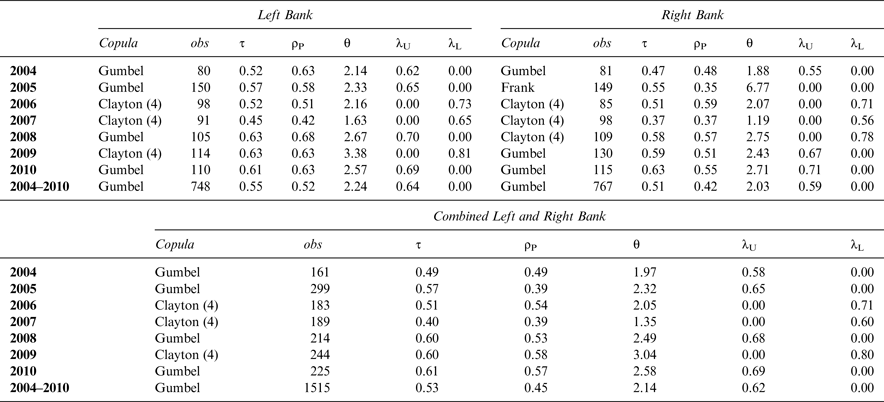
Our results easily conclude that en primeur prices and Parker's ratings exhibit fairly consistent upper-tail dependence in terms of the identified best-fitting copula as being the Gumbel or the transformed-data (Clayton (4)) copula. Only in the case of Right Bank wines in 2005 is the identified best-fitting copula not the Gumbel or the Clayton (4). In that particular case, the Frank copula is best fitting, indicating greater dependence in the middle of the bivariate distribution as opposed to at the tails. When the Left and Right Bank data are combined, all seven years exhibit a high value of tail dependence; when the data are employed across all years, the Gumbel copula is identified for the Left and Right Bank data, jointly and separately.

As previously noted, the upper-tail-dependence parameter represents the conditional probability in the limit that one variable (wine price) exhibits a high value, given a high value in the other variable (critic's rating). In terms of the Left Bank, when the data across all seven years are combined, this conditional probability is 0.64; for the Right Bank, it is 0.59. When the Left and Right Bank data are combined, the conditional probability of a high wine price given a high wine rating is 0.62.

The importance of the upper-tail dependence is also exhibited in terms of the linear-dependence parameters. Kendall's tau and Pearson's correlation coefficient indicate positive correlation ranging, in the case of Pearson's rho from ρ _P  = 0.35 for the 2005 Right Bank data to ρ _P  = 0.68 for the 2008 Left Bank data. However, in all cases (except for the 2005 Right Bank data), the linear-correlation results are driven by nonlinear upper-tail dependence.

B. Marginal-Distribution Identification

As noted previously, the benefit of copula-function modeling is the ability to identify marginal distributions independently from the identification of the copula function. For Parker's ratings and for wine prices, the AIC maximum-likelihood test statistic is employed to identify the most representative probability-distribution function. In the case of Parker's ratings, truncation of the lower tail at a value of 50 and an upper-tail limit of 100 is controlled for, while in the case of wine prices, the distributions are constrained with a truncated lower tail of zero, given non-negative prices. Ninety different possible continuous and discrete probability distributions are considered and ranked in each case using the AIC statistic for Parker's ratings and for wine prices. The results (available from the authors) for the Left and Right Banks and for 2004 through 2010 are consistent. In particular, Parker's ratings exhibit significant negative skewness for each of the years and for the Left and Right Banks, while wine prices exhibit significant positive skewness.

Given the relative stationarity in terms of results for the Right and Left Bank data as well as across years, the combined data of 1,515 observations are employed to identify suitable marginal distributions. The best-fitting distribution functions and their parameters are found to be the Logistic distribution (α = 90.59, β = 2.06) in the case of Parker's ratings and the Generalized Extreme Value (GEV) distribution (a = 26.28, b = 16.65, c = 0.73) in the case of wine prices. The marginal distributions are illustrated in Figure 4, plotted along with the histograms of the 1,515 observations of rating and price data.

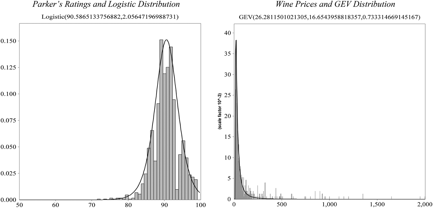
Figure 4 Histogram and Plot of Best-Fitting Distribution for Parker's Ratings and Wine Prices: 2004–2010 Left and Right Banks

C. Monte Carlo Simulation

Employing the Logistic distribution for Parker's ratings, the GEV distribution for prices, and the identified Gumbel copula (θ = 2.13676) based on the combined 2004–2010 Left and Right Bank data, Monte Carlo simulation is used to generate 5,000 observations of Parker's ratings and wine prices. Figure 5 provides a bivariate uniform-distribution plot of the data from the simulation, which indicates primarily upper-tail dependence and slight lower-tail dependence consistent with the Gumbel copula.

Figure 5 Bivariate Uniform-Distribution Plot of Simulated Parker's Ratings and Wine Price Data

Figure 6 shows the plot of the 5,000 simulated Parker's ratings and wine prices, which indicates a strong nonlinear relationship between ratings and prices, consistent with the findings of Noparumpa et al. (Reference Noparumpa, Kazaz and Webster2015).

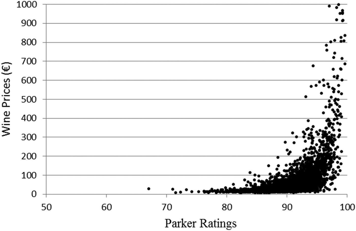
Figure 6 Graph of Simulated Parker's Ratings and Wine Prices

The value of the simulation is in ascertaining the relationship between Parker's ratings and en primeur prices. We categorize the 5,000 simulated data points by ratings, and calculate the Pearson correlation coefficient between ratings and prices in each respective category to provide a more intuitive sense of the relationship. The results, shown in Table 3, provide a practical indication of the nonlinear relationship between the two variables. In particular, some lower-tail dependence is exhibited with a Pearson correlation coefficient of 0.27 in the 75–80 rating range, while the highest correlation is in the 95–100 rating range, with a correlation coefficient of 0.52.

Table 3 Price Average, Standard Deviation, and Price/Rating Correlation for Different Ranges of Parker's Ratings

The review of the impact of expert ratings on wine prices by Oczkowski and Doucouliagos (Reference Oczkowski and Doucouliagos2015) affirms a moderate but significant impact of quality ratings on wine prices; however, our results indicate a significant nonlinearity in the relationship, with the greatest correlation occurring at the positive tail of the bivariate distribution. This result has significant ramifications for producers in determining the potential impact of experts’ ratings on prices.

IV. Conclusions and Future Research

Although Parker is the leading wine critic, he has recently discontinued his provision of barrel ratings (Lyons, Reference Lyons2015). Therefore, further study could include an examination of the nonlinear relationship of wine futures prices to other wine critics’ ratings. The database includes, for example, the wine ratings of 11 other critics, including the renowned Jancis Robinson and Decanter magazine. One approach in terms of further research could include an examination of en primeur prices with respect to an index of ratings. Standardization of wine critics’ ratings is therefore a related issue (Cardebat and Paroissien, Reference Cardebat and Paroissien2015). In addition, a copula-function approach to the relationship between various wine critics’ ratings would be insightful.

Other factors affecting wine prices, such as reputation, could also be explored through more complex multivariate copula-function modeling. Limitations exist, as of yet, in terms of computational complexity. In addition, more complex copula functions, such as the Joe–Clayton copula, could also be employed. This particular copula function could provide a more refined estimate of lower-tail dependence along with the strong upper-tail dependence observed. Clearly, however, upper-tail dependence between Parker's ratings and en primeur prices is the dominant relationship.

Additional opportunities exist for the use of copula-function modeling within the endeavor of viticulture and wine, particularly in terms of weather variables, harvests, and wine quality. These possibilities are evidenced by recent applications in agricultural economics with respect to many other agricultural commodities and the implications for risk management. Other opportunities may also exist in terms of consumer-preference research.