


1. Introduction
There has been a long-standing scientific interest in flexural–gravity waves (also called hydroelastic waves in the literature) due to their importance for marine structures and sea transport. Flexural–gravity waves resulting from the interaction between moving fluids and deformable sheets have a wide range of applications in the polar regions where large floating ice sheets are used as roadways and landing strips. More recently, very large floating structures, such as floating airports (e.g. the Maga-Float project in Tokyo) and ultra-large merchant container vessels were thought to be environmentally friendly and self-sustained for converting ocean waves into energy. A better understanding of large-scale fluid–structure interactions, including flexural–gravity waves, is of fundamental importance in the process of building and utilising these engineering structures.
The study of flexural–gravity waves was initiated by Greenhill (Reference Greenhill1886, Reference Greenhill1916), who obtained the dispersion relation of this new type of wave and proposed the first practical application. Thereafter, flexural–gravity waves and their applications in marine engineering received growing attention from the scientific community. Research findings before the 1990s, most of which are based on linear theories, are summarised in the monograph by Squire et al. (Reference Squire, Hosking, Kerr and Langhorne1996). Observations of intense waves-in-ice events reported by Marko (Reference Marko2003) indicate that nonlinearity may play an important role. The first mathematical result on nonlinear flexural–gravity waves was the computation of large-amplitude periodic waves carried out by Forbes (Reference Forbes1986) via a high-order series truncation method.
However, a key motivation to study nonlinear flexural–gravity waves is the generation of waves as a load moves on an ice cover. The linear theory shows that there exists a critical speed  $c_{min}$ such that, if the speed of the moving load is close to
  $c_{min}$, energy can hardly radiate away from the load. Although the linear theory identifies the critical speed, it fails to describe accurately the wave phenomenon near
  $c_{min}$, since it predicts unlimited growth of wave amplitudes. Părău & Dias (Reference Părău and Dias2002) first performed the weakly nonlinear normal-form analysis for both free and forced problems near
  $c_{min}$, which showed the existence of envelope solitons in shallow fluids that are qualitatively similar to the experimental measurements carried out at Lake Saroma in Hokkaido (Takizawa Reference Takizawa1988). However, their analysis and numerics cannot be generalised to the deep-water case, though a similar critical phenomenon was observed at McMurdo Sound in Antarctica by Squire et al. (Reference Squire, Robinson, Langhorne and Haskell1988). Milewski, Vanden-Broeck & Wang (Reference Milewski, Vanden-Broeck and Wang2011) revisited the problem and showed numerically from the full Euler equations that, even though small-amplitude localised travelling wave solutions are not predicted to exist in deep water by standard perturbation analyses, they do occur along a new type of bifurcation branch.
All the aforementioned nonlinear analyses are based on the nonlinear Kirchhoff–Love plate theory, which has been widely used but does not have a clear conservation form for the elastic potential energy. Most recently, Toland (Reference Toland2007) proposed a model for plates based on the Cosserat theory of hyperelastic shells satisfying Kirchhoff's hypotheses, with the elastic energy being the total squared curvature. Since then, nonlinear flexural–gravity waves with the Toland elastic model have attracted intensive attention. Of interest are the following works: Guyenne & Părău (Reference Guyenne and Părău2012, Reference Guyenne and Părău2014) searched for hydroelastic solitary waves for the full Euler equations using the boundary integral method and performed unsteady simulations by truncating the Dirichlet–Neumann operator in arbitrary depth; Gao & Vanden-Broeck (Reference Gao and Vanden-Broeck2014) investigated the elevation generalised solitary waves in finite depth; Gao, Wang & Vanden-Broeck (Reference Gao, Wang and Vanden-Broeck2016) studied the stability and dynamics of solitary waves for the fully nonlinear equations via a time-dependent conformal mapping technique; and Trichtchenko et al. (Reference Trichtchenko, Milewski, Părău and Vanden-Broeck2019) carried out the linear spectral analysis for periodic waves using the Fourier–Floquet–Hill method and compared the results with those obtained by a modulational instability analysis.
Satellite measurements of ice cover displacements induced by moving vehicles reported by van der Sanden & Short (Reference van der Sanden and Short2017) stress the need for continued efforts in research on three-dimensional fully localised flexural–gravity waves, known as lumps. The nonlinear elastic model in three dimensions was proposed by Plotnikov & Toland (Reference Plotnikov and Toland2011) using the Willmore functional (namely the total squared mean curvature). Milewski & Wang (Reference Milewski and Wang2013) derived the Benney–Roskes–Davey–Stewartson system in the vicinity of the minimum of the phase speed to predict the existence and elucidate the bifurcation mechanism of hydroelastic lumps. Recently, hydroelastic lumps were found numerically for the full Euler equations by Trichtchenko et al. (Reference Trichtchenko, Părău, Vanden-Broeck and Milewski2018) using a boundary integral equation method.
The results mentioned above were obtained for irrotational flows. However, sea surface waves are commonly accompanied by underlying currents, and sometimes the current speed varies with depth (e.g. tidal currents and wind-driven currents). Early numerical works in this direction were carried out by Simmen & Saffman (Reference Simmen and Saffman1985), Teles Da Silva & Peregrine (Reference Teles Da Silva and Peregrine1988), Milinazzo & Saffman (Reference Milinazzo and Saffman1990) and Vanden-Broeck (Reference Vanden-Broeck1994), who computed surface gravity waves for the fully nonlinear equations with constant vorticity. Recently, the cubic nonlinear Schrödinger equation was derived by Thomas, Kharif & Manna (Reference Thomas, Kharif and Manna2012) for pure gravity waves and by Hsu et al. (Reference Hsu, Kharif, Abid and Chen2018) for capillary–gravity waves to investigate the modulational instability of wave trains propagating on a linear shear current. Curtis, Carter & Kalisch (Reference Curtis, Carter and Kalisch2018) expanded the primitive equation to the next asymptotic order to obtain the Dysthe equation with constant vorticity and investigated the motion and mean properties of particle paths. In addition, Hsu et al. (Reference Hsu, Francius, Montalvo and Kharif2016) extended the Stokes expansion to capillary–gravity waves and paid particular attention to the effect of vorticity on the phase velocity, wave profile and Wilton-type waves. On the theoretical side, wave–current interactions have received great attention since the pioneering work by Constantin & Strauss (Reference Constantin and Strauss2004) on local and global bifurcations of periodic gravity waves propagating on an arbitrary vorticity distribution. Subsequent research has focused on particle paths and flow structures beneath free-surface waves in the presence of vorticity. The interested reader is referred to Ehrnström & Villari (Reference Ehrnström and Villari2008), Wahlén (Reference Wahlén2009) and Matioc (Reference Matioc2014) and references therein for more details.
There are relatively fewer studies on the interaction between an underlying current and flexural–gravity waves. This is a special kind of wave–current–structure interaction. Peake (Reference Peake2001, Reference Peake2004) considered the nonlinear stability and the dynamics of a fluid-loaded elastic plate interacting with a mean flow using the method of multiple scales. He showed that the interaction gives interesting phenomena, including negative-energy waves and convective instability. Xia & Shen (Reference Xia and Shen2002) studied flexural–gravity waves in river channels in the presence of a mean flow, and derived the fifth-order Korteweg–de Vries (KdV) equation in the weakly nonlinear shallow-water regime. Bhattacharjee & Sahoo (Reference Bhattacharjee and Sahoo2009) examined the effect of underlying shear currents on flexural–gravity waves in the linear shallow-water approximation. Wave scattering and trapping by jet-like shear currents were both analysed.
For hydroelastic waves with constant vorticity, a cubic nonlinear Schrödinger equation was derived by Gao, Wang & Milewski (Reference Gao, Wang and Milewski2019), together with equations in the resonant cases. Fully nonlinear computations of solitary waves and the study of Benjamin–Feir instabilities were carried out to validate the weakly nonlinear models and to extend their results. Based on the same physical setting (a schematic is shown in figure 1), we focus in the present paper on asymptotics, global bifurcations, new steady solutions and particle trajectories in both periodic and solitary waves, as well as flow structures beneath solitary waves. The numerical computations used in this paper to solve the fully nonlinear equations rely on a conformal mapping method. This is similar to the approaches of Choi (Reference Choi2009), who studied the influence of a linear shear current on the Benjamin–Feir instability of a gravity wave train, and of Ribeiro, Milewski & Nachbin (Reference Ribeiro, Milewski and Nachbin2017), who investigated the flow structure as multiple stagnation points appear due to wave–current interactions.

Figure 1. Sketch of the flow configuration.
The outline of the paper is as follows. The mathematical formulation of the problem is given in § 2. The results for symmetric, periodic and steadily travelling waves, including the third-order Stokes expansion, global bifurcations, generalised solitary waves and wave fronts, and particle trajectories, are presented in § 3. The numerical results for solitary waves are shown in § 4, with particular attention paid to particle paths and streamline patterns beneath the free surface. Finally, § 5 contains our conclusions and further remarks.
2. Governing equations
We consider a two-dimensional incompressible and inviscid fluid of finite depth  $h$ covered by an elastic sheet that provides a restoring force through its bending deformation. We introduce Cartesian coordinates with the
  $x$-axis along undisturbed elastic sheet and the
  $z$-axis directed vertically opposite to gravity. In non-perturbed states, the flow is assumed to be a shear current varying linearly in
  $z$, namely
  $U(z)=U_0+\varOmega _0z$, where
  $U_0$ and
  $\varOmega _0$ are both constants and
  $\varOmega _0$ is called the vorticity strength. There exists a frame of reference where the velocity vanishes at the undisturbed free surface; therefore, without loss of generality, we can let
  $U_0=0$ throughout the paper. Flow perturbations superimposed on the shear are assumed to be irrotational, with a potential function
  $\phi$. Therefore, the governing equations of the problem are
 \begin{gather} \phi_{xx}+\phi_{zz} =0\quad \text{for}\ {-}h < z < \eta, \end{gather}
 \begin{gather}\eta_t-\phi_z+(\phi_x+\varOmega_0\eta)\eta_x=0\quad \text{at}\ z=\eta, \end{gather}
 \begin{gather}\phi_t+\frac{1}{2}|\nabla\phi|^{2}+g\eta+\varOmega_0\eta\phi_x-\varOmega_0\psi+\frac{p}{\rho}=0\quad \text{at}\ z=\eta, \end{gather}
 \begin{gather}\phi_z=0\quad \text{at}\ z=-h, \end{gather}
where  $\eta (x,t)$ is the elevation of the elastic sheet,
  $\rho$ the density of the fluid,
  $p$ the pressure at the top surface and
  $g$ the acceleration due to gravity. We denote by
  $\psi$ the streamfunction satisfying the Cauchy–Riemann equations
  $\psi _z=\phi _x$ and
  $\psi _x=-\phi _z$. Following Toland (Reference Toland2007), the pressure across the elastic sheet is assumed to be
 \begin{equation} p=P_a+D\left(\partial_{ss}\kappa+\frac{\kappa^{3}}{2}\right), \end{equation}
where  $P_a$ is atmospheric pressure,
  $D$ the flexural rigidity,
  $\kappa =\eta _{xx}/(1+\eta _x^{2})^{3/2}$ the curvature of the sheet and
  $s$ the arclength parameter with
  $\partial _s=\partial _x/\sqrt {1+\eta _x^{2}}$.
We study longitudinal progressive waves translating at a constant wave speed  $c$. Waves become steady in a reference frame moving with the speed
  $c$, and the kinematic boundary condition can be written as
 \begin{equation} \psi+\tfrac{1}{2}\varOmega_0\eta^{2}-c\eta=\text{const.}\quad\text{or}\quad (\phi_x+\varOmega_0\eta-c)\eta_x-\phi_z=0. \end{equation}
The pressure equation at  $z=\eta$ can be recast as
 \begin{equation} \frac{1}{2}[(\phi_x+\varOmega_0\eta-c)^{2}+\phi_z^{2}]+g\eta +\frac{D}{\rho}\left(\dfrac{\kappa^{3}}{2}+\partial_{ss}\kappa\right)=B, \end{equation}
where  $B$ is the Bernoulli constant. It is noted that the bulk equation (2.1) and the bottom condition (2.4) are unchanged by changing the reference frame.
3. Periodic waves
3.1. Stokes expansion
An exact solution of (2.1), (2.4), (2.6) and (2.7) is
 \begin{equation} \phi=c x,\quad\psi=c z,\quad\eta=0,\quad B=\frac{c^{2}}{2}, \end{equation}
which is simply a uniform stream with velocity  $c$ and an undisturbed flat free surface. Non-trivial travelling waves can be obtained by perturbing the solution (3.1a–d). To achieve this, we introduce a small parameter
  $\epsilon$, which is a measure of the amplitude of the wave, and write the expansions
 \begin{gather} \phi=cx+\epsilon \phi_1(x,z)+\epsilon^{2}\phi_2(x,z)+\epsilon^{3}\phi_3(x,z)+\cdots, \end{gather}
 \begin{gather}\eta=\epsilon\eta_1(x)+\epsilon^{2}\eta_2(x)+\epsilon^{3}\eta_3(x)+\cdots, \end{gather}
 \begin{gather}c=c_0+\epsilon c_1+\epsilon^{2} c_2+\epsilon^{3}c_3+\cdots, \end{gather}
 \begin{gather}B=B_0+\epsilon B_1+\epsilon^{2} B_2+\epsilon^{3}B_3+\cdots, \end{gather}
where  $B_0=c_0^{2}/2$ and a precise definition of
  $\epsilon$ will be given later. This expansion was pioneered by Stokes (Reference Stokes1847) for pure gravity waves, and now bears the name of the Stokes expansion. It was generalised to capillary–gravity waves by Wilton (Reference Wilton1915) and to flexural–gravity waves by Vanden-Broeck & Părău (Reference Vanden-Broeck and Părău2011). In the presence of a linear shear current, the Stokes expansion was carried out by Kishida & Sobey (Reference Kishida and Sobey1988) for gravity waves and by Hsu et al. (Reference Hsu, Francius, Montalvo and Kharif2016) for capillary–gravity waves.
The difficulty due to the unknown free surface can be overcome by writing the potential function on the free surface as a Taylor series,
 \begin{equation} \phi(x,\eta)=\phi(x,0)+\frac{\partial\phi}{\partial z}(x,0)\eta +\frac{1}{2}\frac{\partial^{2}\phi}{\partial z^{2}}(x,0)\eta^{2}+\cdots, \end{equation}
and expanding the kinematic and dynamic boundary conditions around  $z=0$. Substituting the various expansions into (2.1), (2.4), (2.6) and (2.7) and equating the powers of
  $\epsilon$ leads to a succession of linear systems. The linear system obtained at order
  $\epsilon$ reads
 \begin{gather} \phi_{1,xx}+\phi_{1,zz}=0\quad \text{for}\ {-}h < z < 0, \end{gather}
 \begin{gather}c_0\eta_{1,x}+\phi_{1,z}=0\quad \text{at}\ z=0, \end{gather}
 \begin{gather}(g-\varOmega_0c_0)\eta_1-c_0\phi_{1,x}+\frac{D}{\rho}\eta_{1,xxxx}=B_1-c_0c_1 \quad \text{at}\ z=0, \end{gather}
 \begin{gather}\phi_{1,z}=0\quad \text{at}\ z=-h. \end{gather}
If we assume a periodic surface elevation with a fundamental wavenumber  $k$, the solution to this system takes the form
 \begin{equation} \eta_1=A_{11}\cos(kx),\quad\phi_1=c_0A_{11}\frac{\cosh(k(z+h))}{\sinh(kh)}\sin(kx), \end{equation}
with  $B_1=c_0c_1$, where
  $c_0$ satisfies the linear dispersion relation
 \begin{equation} k\coth(kh)c_0^{2}+\varOmega_0c_0-\left(g+\frac{D}{\rho}k^{4}\right)=0, \end{equation}
and  $c_1$ will be determined at the next order in
  $\epsilon$.
At the second order in  $\epsilon$, we have the following sequence of equations:
 \begin{equation} \phi_{2,xx}+\phi_{2,zz}=0\quad \text{for}\ {-}h < z < 0, \end{equation}
 \begin{equation} c_0\eta_{2,x}+\phi_{2,z}=-c_1\eta_{1,x}+\varOmega_0\eta_1\eta_{1,x}+\eta_{1,x}\phi_{1,x}-\eta_1 \phi_{1,zz}\quad \text{at}\ z=0, \end{equation}
 \begin{align}
&(g-\varOmega_0c_0)\eta_2-c_0\phi_{2,x}+\frac{D}{\rho}\eta_{2,xxxx} =
B_2-\frac{c_1^{2}}{2}-c_0c_2+\varOmega_0c_1\eta_1 \nonumber\\ &\quad
-\frac{1}{2}\varOmega_0^{2}\eta_1^{2}-\frac{1}{2}\phi_{1,x}^{2}-\frac{1}{2}\phi_{1,z}^{2}
+c_1\phi_{1,x}-\varOmega_0\eta_1\phi_{1,x}+c_0\eta_1\phi_{1,xz}\quad
\text{at}\ z=0, \end{align}
\begin{align}
&(g-\varOmega_0c_0)\eta_2-c_0\phi_{2,x}+\frac{D}{\rho}\eta_{2,xxxx} =
B_2-\frac{c_1^{2}}{2}-c_0c_2+\varOmega_0c_1\eta_1 \nonumber\\ &\quad
-\frac{1}{2}\varOmega_0^{2}\eta_1^{2}-\frac{1}{2}\phi_{1,x}^{2}-\frac{1}{2}\phi_{1,z}^{2}
+c_1\phi_{1,x}-\varOmega_0\eta_1\phi_{1,x}+c_0\eta_1\phi_{1,xz}\quad
\text{at}\ z=0, \end{align}
 \begin{equation} \phi_{2,z}=0\quad \text{at}\ z=-h. \end{equation}
Eliminating the secular term yields  $c_1=0$ and hence
  $B_1=c_0c_1=0$. Solving for other modes yields
 \begin{gather} \eta_2=A_{22}\cos(2kx),\quad\phi_2=C_{22}\cosh(2k(z+h))\sin(2kx), \end{gather}
 \begin{gather} B_2=c_0c_2+\frac{1}{4}\left[\varOmega_0^{2}+2k\varOmega_0c_0\coth(kh) +\frac{k^{2}c_0^{2}}{\sinh^{2}(kh)}\right]A_{11}^{2}, \end{gather}
where
 \begin{gather} A_{22}=\frac{\coth(2kh)c_0F_{22}+G_{22}} {g+16Dk^{4}/\rho-\varOmega_0c_0-2k\coth(2kh)c_0^{2}}, \end{gather}
 \begin{gather}C_{22}=\frac{(g+16Dk^{4}/\rho-\varOmega_0c_0)F_{22}+2kc_0G_{22}} {2k\sinh(2kh)[g+16Dk^{4}/\rho-\varOmega_0c_0-2k\coth(2kh)c_0^{2}]}, \end{gather}
with
 \begin{gather} F_{22}=-\left[\frac{k\varOmega_0}{2}+c_0k^{2}\coth(kh)\right]A^{2}_{11}, \end{gather}
 \begin{gather}G_{22}=-\tfrac{1}{4}[\varOmega_0^{2}+2c_0k\coth(kh)\varOmega_0 +c_0^{2}k^{2}\coth^{2}(kh)-3c_0^{2}k^{2}]A^{2}_{11}. \end{gather}
It is noted that the Stokes expansion is valid provided that the denominators of  $A_{22}$ and
  $C_{22}$ are non-zero. However, if
 \begin{equation} g+(\kern0.13em jk)^{4}D/\rho-\varOmega_0c_0-(\kern0.13em jk)\coth(\kern0.13em jkh)c_0^{2}=0 \quad \textrm{for}\ j\neq 1, \end{equation}
then the expansion needs to be modified to include two modes:  $k$ and
  $jk$ (the interested reader is referred to Vanden-Broeck & Părău (Reference Vanden-Broeck and Părău2011) for more details). This was first achieved by Wilton (Reference Wilton1915) for capillary–gravity waves, who provided evidence for the non-uniqueness of periodic water waves.
In the same vein, by collecting the terms of  $O(\epsilon ^{3})$ we obtain
 \begin{equation} \phi_{3,xx}+\phi_{3,zz}=0\quad \text{for}\ {-}h < z < 0, \end{equation}
 \begin{align} c_0\eta_{3,x}+\phi_{3,z} &=-c_2\eta_{1,x}+\varOmega_0\eta_{1,x}\eta_2+\varOmega_0\eta_{2,x}\eta_1 -\phi_{1,zz}\eta_2-\phi_{2,zz}\eta_1 \nonumber\\ & \quad -\tfrac{1}{2}\phi_{1,zzz}\eta_1^{2}+\phi_{1,x}\eta_{2,x} +\phi_{2,x}\eta_{1,x}+\phi_{1,xz}\eta_{1,x}\eta_1\quad \text{at}\ z=0, \end{align}
 \begin{align}
&(g-\varOmega_0c_0)\eta_3-c_0\phi_{3,x}+\frac{D}{\rho}\eta_{3,xxxx}
=B_3-c_0c_3+\varOmega_0c_2\eta_1-\varOmega_0^{2}\eta_1\eta_2
-\phi_{1,z}\phi_{2,z}\nonumber\\ &\quad
-\phi_{1,z}\phi_{1,zz}\eta_1+c_2\phi_{1,x}
-\varOmega_0\phi_{1,x}\eta_2-\varOmega_0\phi_{2,x}\eta_1
-\phi_{1,x}\phi_{2,x} - \varOmega_0\phi_{1,xz}\eta_1^{2}+c_0\phi_{1,xz}\eta_2 \nonumber\\
& \quad -\phi_{1,x}\phi_{1,xz}\eta_1
+c_0\phi_{2,xz}\eta_1+\frac{1}{2}c_0\phi_{1,xzz}\eta_1^{2}\quad
\text{at}\ z=0, \end{align}
\begin{align}
&(g-\varOmega_0c_0)\eta_3-c_0\phi_{3,x}+\frac{D}{\rho}\eta_{3,xxxx}
=B_3-c_0c_3+\varOmega_0c_2\eta_1-\varOmega_0^{2}\eta_1\eta_2
-\phi_{1,z}\phi_{2,z}\nonumber\\ &\quad
-\phi_{1,z}\phi_{1,zz}\eta_1+c_2\phi_{1,x}
-\varOmega_0\phi_{1,x}\eta_2-\varOmega_0\phi_{2,x}\eta_1
-\phi_{1,x}\phi_{2,x} - \varOmega_0\phi_{1,xz}\eta_1^{2}+c_0\phi_{1,xz}\eta_2 \nonumber\\
& \quad -\phi_{1,x}\phi_{1,xz}\eta_1
+c_0\phi_{2,xz}\eta_1+\frac{1}{2}c_0\phi_{1,xzz}\eta_1^{2}\quad
\text{at}\ z=0, \end{align}
 \begin{equation} \phi_{3,z}=0\quad \text{at}\ z=-h. \end{equation}
Eliminating the secular term yields
 \begin{align} c_2 &= \left\{\left[2\varOmega_0^{2}+4c_0k\varOmega_0\coth(kh) +\frac{2c_0^{2}k^{2}}{\sinh^{2}(kh)}\right]A_{22} \right. \nonumber\\ &\quad+ [3c_0k^{2}\varOmega_0+4c_0^{2}k^{3}\coth(kh)]A^{2}_{11} +4[2c_0k^{2}\cosh^{2}(kh)\coth(kh) \nonumber\\ &\quad +k\varOmega_0\cosh(2kh)]C_{22}\left. \vphantom{\frac{2c_0^{2}k^{2}}{\sinh^{2}(kh)}}\right\}\left. \vphantom{\frac{2c_0^{2}k^{2}}{\sinh^{2}(kh)}}\right/[4\varOmega_0+8c_0k\coth(kh)]. \end{align}
Solving for non-resonant modes gives
 \begin{gather} \eta_3=A_{33}\cos(3kx), \end{gather}
 \begin{gather}\phi_3=C_{31}\sin(kx)\cosh(k(z+h))+C_{33}\sin(3kx)\cosh(3k(z+h)), \end{gather}
where
 \begin{gather} C_{31}=\frac{c_2A_{11}-\tfrac 38k^{2}c_0A_{11}^{3}-\tfrac 12kc_0A_{11}A_{22}\coth(kh) -kA_{11}C_{22}\cosh(2kh)-\tfrac 12\varOmega_0A_{11}A_{22}}{\sinh(kh)}, \end{gather}
 \begin{gather}A_{33}=\frac{\coth(3kh)c_0F_{33}+G_{33}} {g+81k^{4}D/\rho-\varOmega_0c_0-3k\coth(3kh)c_0^{2}}, \end{gather}
 \begin{gather}C_{33}=\frac{(g+81k^{4}D/\rho-\varOmega_0c_0)F_{33}+3kc_0G_{33}} {3k\sinh(3kh)[g+81k^{4}D/\rho-\varOmega_0c_0-3k\coth(3kh)c_0^{2}]}, \end{gather}
with
 \begin{equation} F_{33}=-\tfrac{3}{2}[k\varOmega_0+c_0k^{2}\coth(kh)]A_{11}A_{22} -\tfrac{3}{8}c_0k^{3}A^{3}_{11}-3k^{2}\cosh(2kh)A_{11}C_{22}, \end{equation}
 \begin{align} G_{33}&=-\frac{\varOmega_0^{2}}{2}A_{11}A_{22}-\frac{k\varOmega_0}{4} [c_0kA_{11}^{2}+2c_0\coth(kh)A_{22}+4\cosh(2kh)C_{22}]A_{11} \nonumber\\ &\quad +\frac{c_0k^{2}}{8} [16\sinh(2kh)C_{22}-8\coth(kh)C_{22}+c_0k\coth(kh)A_{11}^{2}+4c_0A_{22}]A_{11}. \end{align}
In addition,  $B_3=c_0c_3$ and the next order of
  $\epsilon$ gives
  $B_3=c_3=0$.
Upon noticing that
 \begin{equation} \eta(x)=\epsilon A_{11}\cos(kx)+\epsilon^{2}A_{22}\cos(2kx)+\epsilon^{3}A_{33}\cos(3kx)+\cdots, \end{equation}
we denote by  $a$ the first Fourier coefficient of
  $\eta (x)$, i.e.
 \begin{equation} a=\frac{2}{\lambda}\int_{-\lambda/2}^{\lambda/2}\eta(x)\cos(kx)\,\mathrm{d}x=\epsilon A_{11}. \end{equation}
Following Vanden-Broeck (Reference Vanden-Broeck2010), if we define the parameter  $\epsilon$ as
  $\epsilon ={a}/{\lambda }$, it then follows that
  $A_{11}=\lambda$.
In the discussion above, we carried out the Stokes expansion to the third order, which results in a correction to the linear speed of wave propagation since  $c_1=0$ and
  $c_2\neq 0$. This procedure was previously applied by Kishida & Sobey (Reference Kishida and Sobey1988) and Hsu et al. (Reference Hsu, Francius, Montalvo and Kharif2016) in different contexts. As a check, we compare
  $c_2$ with the value from Hsu et al. (Reference Hsu, Francius, Montalvo and Kharif2016) when only gravity is considered (i.e. taking
  $p=\text {const.}$ in (2.3)). It turns out that, under this circumstance, (3.28) can be reduced to
 \begin{align} c_2 &= \frac{k c_0^{2}}{8[2+\varOmega_0\sigma]} \left[\frac{\varOmega_0^{4}}{k^{4}c_0^{4}}+\frac{(6+2\sigma^{2})\varOmega_0^{3}}{k^{3}c_0^{3}\sigma} +\frac{(15+3\sigma^{2})\varOmega_0^{2}}{k^{2}c_0^{2}\sigma^{2}} \right. \nonumber\\ &\quad\left.+\frac{(18-4\sigma^{2}+2\sigma^{4})\varOmega_0}{kc_0\sigma^{3}} +\frac{9-10\sigma^{2}+9\sigma^{4}}{\sigma^{4}}\right], \end{align}
where  $\sigma =\tanh (kh)$ and we have used
  $1/k$,
  $\varOmega _0\sqrt {gk}$ and
  $c_0\sqrt {g/k}$ to replace
  $A_{11}$,
  $\varOmega _0$ and
  $c_0$, respectively, for comparison purpose. Equation (3.38) is exactly the same as (3.32) in Hsu et al. (Reference Hsu, Francius, Montalvo and Kharif2016) when surface tension is neglected, providing a partial verification for our calculation.
3.2. Validation
We start with comparing the asymptotic results of the Stokes expansion with numerical solutions of the full Euler equations. To seek travelling waves for (2.1)–(2.4), we first non-dimensionalise the system by choosing
 \begin{equation} \left[\frac{D}{\rho g}\right]^{1/4}, \quad \left[\frac{D}{\rho g^{5}}\right]^{1/8} \quad\text{and}\quad \left[\frac{g D^{3}}{\rho^{3}}\right]^{1/8} \end{equation}
as the units of length, time and potential, respectively. Therefore, the coefficients  $g$ and
  $D/\rho$ are equal to 1 in (2.7), and
  $\varOmega _0$ in (2.6) and (2.7) can be replaced by a non-dimensional vorticity strength
  $\varOmega$ defined as
 \begin{equation} \varOmega=\left(\frac{D}{\rho g^{5}}\right)^{1/8}\varOmega_0. \end{equation}
 Following Gao et al. (Reference Gao, Wang and Milewski2019), the problem can be handled by using a conformal transformation that maps the physical fluid domain to a strip in a complex plane. For travelling waves, after the transformation the unknown free surface can be parametrised by  $\eta (\xi )$, which satisfies an integro-differential equation
 \begin{equation} \frac{1}{2J}(\varOmega\eta x_\xi+\varOmega\mathcal{T}[\eta\eta_\xi]-c)^{2} +\eta+\frac{1}{2}\left[\frac{\kappa_{\xi\xi}}{J} +\left(\frac{\kappa_\xi}{J}\right)_\xi+\kappa^{3}\right]=B, \end{equation}
where  $x_\xi =1-\mathcal {T}[\eta _\xi ]$,
  $J=x_\xi ^{2}+\eta _\xi ^{2}$ is the Jacobian of the map, and the curvature
  $\kappa$ in the new plane is of the form
 \begin{equation} \kappa=\frac{\eta_{\xi\xi}x_\xi-x_{\xi\xi}\eta_\xi}{J^{3/2}}. \end{equation}
It is noted that the translating speed  $c$ and the Bernoulli constant
  $B$ are also unknowns and need to be determined together with
  $\eta (\xi )$. The detailed derivation of (3.41) can be found, for example, in Gao et al. (Reference Gao, Wang and Milewski2019).
The pseudo-differential operator  $\mathcal {T}$ is defined as
 \begin{equation} \mathcal{T}[f]=\frac{1}{2\tilde{h}}\int_{-\lambda/2}^{\lambda/2} \,f(\xi')\coth\left[\frac{\rm \pi}{2\tilde{h}}(\xi'-\xi)\right]\,\textrm{d}\xi', \end{equation}
where  $\lambda$ is the wavelength and
  $\tilde {h}$ is the thickness of the fluid in the transformed plane defined as
 \begin{equation} \tilde{h}=h+\frac{1}{\lambda}\int_{-\lambda/2}^{\lambda/2}\eta(\xi)\,\textrm{d}\xi. \end{equation}
We approximate  $\eta (\xi )$ by the truncated Fourier series
 \begin{equation} \eta(\xi)=\sum_{n=-N}^{N}a_n\exp({\textrm{i}2{\rm \pi} n\xi/\lambda}), \end{equation}
where  $a_n$ are real and
  $a_n=a_{-n}$ due to symmetry. We introduce collocation points uniformly distributed along the
  $\xi$-axis. This provides discrete algebraic equations by projecting (3.41) onto each Fourier mode. The equations are solved by Newton's method with the classical pseudo-spectral algorithm. To obtain solutions with high accuracy, a large number of Fourier modes is used in the computation (typically 1024 modes are sufficient for periodic waves) and solutions are considered exact if increasing the number of Fourier modes does not change the solutions within graphical accuracy. The solution was considered to have converged when the
  $l^{\infty }$-norm of the residual error is less than
  $10^{-10}$.
The parameter space consists of four dimensionless parameters: the vorticity strength  $\varOmega$, the fluid depth
  $h$, the wave speed
  $c$, and the wavelength
  $\lambda$ (or, equivalently, the wavenumber
  $k$). To obtain more solutions or complete bifurcation curves, we use continuation methods where one previously computed solution is used as an initial guess to compute a new solution for slightly perturbed values of the parameters. The validity and accuracy of such schemes have been checked by several groups, and the interested reader is referred to Vanden-Broeck (Reference Vanden-Broeck1994), Choi (Reference Choi2009) and Gao et al. (Reference Gao, Wang and Milewski2019) and references therein for more details.
We now use both numerical results for the full Euler equations and asymptotic predictions from the Stokes expansion to compare periodic travelling wave solutions. The asymptotic solutions can be obtained by substituting the expressions of  $\phi _i$,
  $\eta _i$,
  $c_i$ and
  $B_i$ into (3.2)–(3.5), choosing
  $A_{11}=\lambda$, and varying the value of
  $\epsilon$. Figure 2 illustrates the comparison between the asymptotic and numerical solutions for different values of
  $\epsilon$. As expected, the difference between asymptotic predictions and numerical results increases as the wave steepness increases. As opposed to downstream waves (
 $\varOmega c>0$, shown in figure 2a,c), steeper waves exist in the upstream case (
 $\varOmega c<0$, shown in figure 2b,d), and the third-order approximation still works well for moderate-amplitude waves. It is observed that the downstream waves have a flat and wide crest while the upstream waves feature a narrow crest.

Figure 2. Comparison of surface profiles between the Stokes theory and numerical solutions of the fully nonlinear equations. The computed solutions are shown by solid lines, and the third-order approximate solutions are plotted by dashed lines.  $(a{,}c)$ Wave profiles when the parameters are chosen as
  $h=5$,
  $\lambda =4{\rm \pi}$ and
  $\varOmega =1$ with (a)
  $\epsilon =0.0118$ and (c)
  $\epsilon =0.0444$.
  $(b{,}d)$ Wave profiles when the parameters are chosen as
  $h=1$,
  $\lambda =4{\rm \pi}$ and
  $\varOmega =7$ with (b)
  $\epsilon =0.0275$ and (d)
  $\epsilon =0.0565$.
To second order, the Stokes expansion predicts that the wave speed is independent of the wave amplitude since  $c_1=0$. At third order, the asymptotic expansion gives a correction
  $c_2$ to the linear phase velocity. In figure 3, wave speeds predicted by the third-order Stokes theory (dashed lines) and the fully nonlinear numerical computations (solid lines) are compared. Six solution branches for various values of
  $\varOmega$ are presented. It is shown that the asymptotic wave speeds match the numerical results very well for small- and moderate-amplitude waves. We stop continuing the branches when Newton's method diverges or oscillates and fails to reach the desired accuracy. Wave profiles corresponding to the right endpoints of these curves are presented in figure 4, where the numerical results are shown as solid lines and the asymptotic predictions are shown as dashed lines. In general, the Stokes expansion works well for moderate-amplitude waves except for the case of zero vorticity, where the third-order solution is a poor approximation of the numerical solution, as shown in figure 4(c). If we check the denominator of
  $A_{22}$, it is found that
  $1+16k^{4}-2\coth (2kh)c_0^{2}\approx -0.05$ and the situation is very close to resonant harmonics or Wilton ripples, which explains the poor performance of the Stokes expansion in such a case.

Figure 3. Speed–amplitude diagram for different values of  $\varOmega$. The figure shows the comparison of the wave speed between the Stokes theory and the numerical solutions of the fully nonlinear equations. The computed solutions are shown by solid lines, and the third-order approximate results are given by dashed lines. The parameters are chosen as
  $h=4$ and
  $\lambda =4{\rm \pi}$. From top to bottom,
  $\varOmega =-2$,
  $-1$,
$-1$,  $0$,
$0$,  $0.5$,
  $1$ and
  $2$, and the wave slopes of the computed solutions (defined by
  $2[\eta (0)-\eta (\lambda /2)]/\lambda$) at the termination points read
  $0.1273$,
  $0.1464$,
  $0.0875$,
  $0.1194$,
  $0.1210$ and
  $0.1114$, respectively.

Figure 4. Wave profiles corresponding to the right endpoints of the curves shown in figure 3. The computed solutions are shown by solid lines and the third-order approximate results are plotted by dashed lines for  $h=4$,
  $\lambda =4{\rm \pi}$ and:
  $(a)$
$(a)$  $\varOmega =-2$,
  $\epsilon =0.0318$;
  $(b)$
$(b)$  $\varOmega =-1$,
  $\epsilon =0.0365$;
  $(c)$
$(c)$  $\varOmega =0$,
  $\epsilon =0.023$;
  $(d)$
$(d)$  $\varOmega =0.5$,
  $\epsilon =0.0285$;
  $(e)$
$(e)$  $\varOmega =1$,
  $\epsilon =0.0285$; and
  $(\,f)$
  $\varOmega =2$,
  $\epsilon =0.0249$.
3.3. Global bifurcation
In this subsection we study the global bifurcation of periodic waves of the fully nonlinear equations. To avoid taking into account the effects of all the parameters, we fix  $\varOmega$,
  $h$ and
  $k$, where
  $\varOmega$ is chosen to be non-zero to include vorticity effects, and explore the wave speed–amplitude relationship. We start from the flat state and compute a branch of solutions until it returns to a trivial or stationary solution, termed a global bifurcation in the current paper. It is obvious that changing the signs of
  $\varOmega$ and
  $c$ simultaneously in (3.41) results in the same equation, hence we only need to consider positive
  $\varOmega$. Furthermore, numerical evidence shows that the profiles and the bifurcations are much richer for upstream waves (waves propagating against the background shear). Therefore, we choose
  $\varOmega >0$ and
  $c<0$ in the following numerical calculations.
A small-amplitude monochromatic wave with propagating speed satisfying the linear dispersion relation is used as the initial guess for Newton's method. After iterating to a solution of the nonlinear integro-differential equation (3.41) within a desired tolerance, a continuation method is used to search for more solutions along the same branch by perturbing the previously computed solution by a small amount in some bifurcation parameter. The translating speed  $c$, the value of the centre point of the free-surface displacement
  $\eta (0)$, and the wave amplitude, which is defined as
 \begin{equation} H:=\eta(0)-\eta(\lambda/2), \end{equation}
are used as bifurcation parameters to complete the bifurcation curves. It is noted that solutions with an overhanging structure are allowed in our computations due to the formulation of water waves in holomorphic coordinates. We stop the computation when the solution reaches the boundary of the speed–amplitude diagram (i.e. the wave becomes either a free stream or a stationary profile).
An example of a global bifurcation branch of waves, which terminates in one endpoint at  $c=0$ and another at
  $H=0$, is shown in figure 5. We start from small-amplitude waves and increase
  $H$ to trace the branch. Then
  $\eta (0)$ is used as the continuation parameter to traverse the very sharp turning point labelled
 ![]() on the curve. Finally, we vary the wave speed to complete the bifurcation diagram. The most striking phenomenon observed in this example is the closing of the overhanging structure and its reopening. Akers et al. (Reference Akers, Ambrose, Pond and Wright2016) and Akers, Ambrose & Sulon (Reference Akers, Ambrose and Sulon2017) numerically investigated the global bifurcation of interfacial hydroelastic waves based on the Birkhoff–Rott integral and arclength parametrisation. Their formulation for water-wave problems also allows multivalued wave profiles. However, they had to stop the computation at a limiting configuration where a self-intersecting point appears, enclosing a pendant-shaped bubble. In this situation, in contrast to their results, we can still continue the branch by changing some bifurcation parameter (speed or amplitude), taking advantage of conformal mapping, even though solutions with multiple intersecting points are non-physical (see
on the curve. Finally, we vary the wave speed to complete the bifurcation diagram. The most striking phenomenon observed in this example is the closing of the overhanging structure and its reopening. Akers et al. (Reference Akers, Ambrose, Pond and Wright2016) and Akers, Ambrose & Sulon (Reference Akers, Ambrose and Sulon2017) numerically investigated the global bifurcation of interfacial hydroelastic waves based on the Birkhoff–Rott integral and arclength parametrisation. Their formulation for water-wave problems also allows multivalued wave profiles. However, they had to stop the computation at a limiting configuration where a self-intersecting point appears, enclosing a pendant-shaped bubble. In this situation, in contrast to their results, we can still continue the branch by changing some bifurcation parameter (speed or amplitude), taking advantage of conformal mapping, even though solutions with multiple intersecting points are non-physical (see ![]() in figure 5).
in figure 5).

Figure 5. Amplitude–speed bifurcation diagram for periodic waves with  $h=5$,
  $\lambda =2{\rm \pi}$ and
  $\varOmega =1$. Typical wave profiles labelled
 ![]() on the bifurcation curve, corresponding to
on the bifurcation curve, corresponding to  $c=-2.05$,
  $-2.73$,
  $-1.91$ and
  $-0.74$, respectively, are also plotted.
A global bifurcation curve can connect two trivial solutions with different propagating speeds. It is shown in figure 6 that a branch of waves with a wavelength of  ${\rm \pi}$ (dashed line) intersects with the
  $4{\rm \pi}$-period branch (solid line) at point
 ![]() on the curve. Following the path
on the curve. Following the path ![]() –
–![]() and starting from point
and starting from point ![]() , figure 7 provides a sequence of profiles that illustrate how a profile with four crests gradually emerges. We compute the solution with the period of
, figure 7 provides a sequence of profiles that illustrate how a profile with four crests gradually emerges. We compute the solution with the period of  ${\rm \pi}$ at the same speed (circles in figure 7d), which is exactly on top of the
  $4{\rm \pi}$-period solution (solid line in figure 7d), confirming our observations. It is also found in figure 6 that the
  $4{\rm \pi}$-period branch forms a closed loop. Waves on one half of the branch are the same as those on the other half but with a phase shift of
  $2{\rm \pi}$. One-and-a-half periods of solutions
 ![]() and
and ![]() are plotted together in figure 7(c) to clearly demonstrate the phenomenon of phase shift.
are plotted together in figure 7(c) to clearly demonstrate the phenomenon of phase shift.

Figure 6. Bifurcation diagrams of hydroelastic periodic waves with  $h=5$ and
  $\varOmega =1$, but with different wavelengths. The
  $4{\rm \pi}$-period solution branch is shown by solid curves, while the
  ${\rm \pi}$-period branch is plotted as a dashed curve. These two branches both bifurcate from zero amplitude (labelled with stars) and intersect each other at point
 ![]() , where they have exactly the same wave profiles.
, where they have exactly the same wave profiles.

Figure 7. Typical wave profiles that correspond to ![]() –
–![]() shown in figure 6. The solid curves in (a–d) correspond to
shown in figure 6. The solid curves in (a–d) correspond to ![]() –
–![]() , respectively. Point
, respectively. Point ![]() is shown by a dashed curve in
is shown by a dashed curve in  $(c)$, which is the same as
 ![]() except for a phase shift of
except for a phase shift of  $2{\rm \pi}$. The
  ${\rm \pi}$-period solution on the dashed curve at point
 ![]() in figure 6 is shown by circles in
in figure 6 is shown by circles in  $(d)$, which exactly matches the
  $4{\rm \pi}$-period solution.
3.4. Generalised solitary waves and fronts
Generalised solitary waves are nonlinear non-periodic travelling waves with a central core similar to a classical solitary pulse and a non-decaying train of ripples extending up to infinity. Generalised solitary waves were previously computed by, among others, Hunter & Vanden-Broeck (Reference Hunter and Vanden-Broeck1983) and Champneys, Vanden-Broeck & Lord (Reference Champneys, Vanden-Broeck and Lord2002) for capillary–gravity waves and by Gao & Vanden-Broeck (Reference Gao and Vanden-Broeck2014) for flexural–gravity waves; all the computations were carried out in periodic domains (in other words, the generalised solitary waves were approximated by long periodic waves in numerics). Proofs of the existence of generalised capillary–gravity solitary waves were provided by Beale (Reference Beale1991) and others.
We now compute periodic waves with non-decaying oscillatory tails akin to generalised solitary waves for downstream flexural–gravity waves. We take a long small-amplitude cosine function ( $k\approx 0.1$ say) as the initial guess for the Newton–Raphson iteration and use the amplitude or speed as the bifurcation parameter. As the amplitude increases, the solution gradually approaches the configuration of a solitary pulse in the middle with several periodic waves in the tails (see figure 8). Further numerical experiments show that the algorithm appears to converge well if we add more and more oscillations to the obtained profile as the initial guess. It is shown in figure 8(a) that the profile obtained for the wavelength
  $\lambda =96.96$ is almost exactly on top of the profile for
  $\lambda =127.19$, which provides strong evidence for the existence of true generalised solitary waves.

Figure 8. Numerical evidence for the existence of generalised solitary waves. The parameters are chosen as  $h=10$ and
  $\varOmega =2$ with:
  $(a)$
$(a)$  $\lambda =96.96$,
  $c=0.5180$ (thick line) and
  $\lambda =127.19$,
  $c=0.5358$ (thin line); and
  $(b)$
$(b)$  $\lambda =132.28$,
  $c=0.4766$ (thick line) and
  $\lambda =209.44$,
  $c=0.4346$ (thin line). Panel
  $(b)$ shows the broadening of the central core leading to a table-top structure.
On the other hand, when we use the wavelength as the bifurcation parameter, the broadening phenomenon of the central core is found. It is observed in figure 8(b) that the central core is flat and becomes broader as  $\lambda$ increases. This solution can even serve as a good approximation for a true solitary wave if we split the wave profile down the middle and glue the two endpoints together, considering the periodic nature of the computational domain (see figure 9a,b). As we enlarge the domain, the coexistence of the two phenomena, namely, the increase in the number of periodic waves in the tails and the broadening of the main core, implies the existence of wave fronts, which were previously only found in interfacial waves in multilayer fluid systems.

Figure 9. Solitary waves with oscillating pulse and wave fronts with various sets of parameters. For  $h=5$ and
  $\varOmega =3$, small-amplitude solutions are shown in (a,c), while moderate-amplitude solutions are shown in (b,d). The computational domains and wave speeds are as follows:
  $(a)$
$(a)$  $\lambda =604.15$,
  $c=0.3237$ (thick line) and
  $\lambda =604.15$,
  $c=0.3268$ (thin line);
  $(b)$
$(b)$  $\lambda =314.16$,
  $c=0.2$ (thick line) and
  $\lambda =314.16$,
  $c=0.2038$ (thin line);
  $(c)$
$(c)$  $\lambda =339.63$,
  $c=0.3237$ (thick line) and
  $\lambda =502.65$,
  $c=0.3338$ (thin line); and
  $(d)$
$(d)$  $\lambda =223.60$,
  $c=0.2$ (thick line) and
  $\lambda =276.79$,
  $c=0.2593$ (thin line).
Wave fronts in hydrodynamics often occur in the flow of contiguous homogeneous fluids of different densities, which are usually called internal fronts. Interfacial gravity solitary waves under the rigid-lid approximation were computed by Turner & Vanden-Broeck (Reference Turner and Vanden-Broeck1988), and the most striking feature found in their work is the broadening of the wave, namely, the midsection of the interface develops a plateau, which becomes infinitely long when the wave speed approaches a limiting value. This numerical result provides evidence for fronts, since broad solitary waves can be viewed as the superposition of two fronts. Dias & Vanden-Broeck (Reference Dias and Vanden-Broeck2003) later showed that, in the limiting configuration, the flow in the far field and the flow in the middle can be referred to as parallel conjugate flows, and the wave indeed becomes a front. Fochesato, Dias & Grimshaw (Reference Fochesato, Dias and Grimshaw2005) proposed a coupled KdV system for multilayer fluids to combine generalised solitary waves and fronts, and they found that ripples can appear on one side of the wave front.
According to the above argument, we consider these solutions as solitary waves with many oscillations in the central core. In figure 9, the possibility of an increase in the number of ripples in the midsection of solitary waves is shown for both small- and moderate-amplitude solutions (see figure 9a,b). More obviously, if we consider half of the solutions, figure 9(c,d) provides strong evidence for the existence of wave fronts, since both flat tails and oscillations in the centre can be extended. The wave profiles shown in figures 8 and 9 are qualitatively similar to the travelling dispersive shock waves (TDSWs) found by Hoefer, Smyth & Sprenger (Reference Hoefer, Smyth and Sprenger2019) and Sprenger & Hoefer (Reference Sprenger and Hoefer2017, Reference Sprenger and Hoefer2020) in the fifth-order KdV equation and related models. As pointed out in their papers, TDSWs feature a partial non-monotonic solitary wave at the trailing edge connected with a periodic travelling wave train, and can be interpreted as nonlinear resonance between different types of nonlinear waves moving with the same speed. However, to the best of the authors’ knowledge, this is the first time that wave fronts in the free-surface Euler equations have been reported.
3.5. Particle trajectories
In this subsection, we calculate particle trajectories numerically for the fully nonlinear equations and compare the results with asymptotic approximations. The particle paths under nonlinear and periodic water waves were initially considered by Stokes (Reference Stokes1847) in his seminal work for irrotational flows and pure gravity waves. He showed that, in contrast to the linear theory, the particle path in the laboratory frame is not a closed loop but features a slight forward drift in the horizontal direction after a wave period has elapsed. This is known as the Stokes drift. A recent breakthrough on the theoretical side of this topic was made by Constantin (Reference Constantin2006), who generalised Stokes’ asymptotic work to steep waves to gain a qualitative understanding of the transport properties of arbitrary Stokes waves based on a rigorous mathematical argument. However, considering the boundary layers at the bottom and at the free surface, recirculation orbits (a phenomenon similar to the particle dynamics of a Gerstner wave) were shown to exist by the asymptotic work of Longuet-Higgins (Reference Longuet-Higgins1953) and the experimental research of Grue & Kolaas (Reference Grue and Kolaas2017). The existence of closed orbits was also proved by Constantin & Strauss (Reference Constantin and Strauss2010) when an underlying mean flow exists, which is intuitively understandable since the forward Stokes drift can be eliminated by the counter-propagating uniform current.
When a linear sheared current is added, theoretical studies on particle paths under periodic gravity waves have only been carried out for waves of arbitrarily small amplitude (Ehrnström & Villari Reference Ehrnström and Villari2008; Wahlén Reference Wahlén2009). On the numerical side, Ribeiro et al. (Reference Ribeiro, Milewski and Nachbin2017) investigated particle trajectories under nonlinear periodic travelling waves with multiple stagnation points in a frame moving with the wave speed, and two dynamic behaviours of fluid particles were observed: periodic transport trajectory and closed orbit.
We start by describing the numerical scheme used to trace the trajectory of a fluid particle. In the frame of reference moving with the wave, particle trajectories can be obtained by solving the following ordinary differential equations:
 \begin{equation} \dfrac{\mathrm{d}x}{\mathrm{d}t}=\phi_{x}+\varOmega z-c,\quad\dfrac{\mathrm{d}z}{\mathrm{d}t}=\phi_{z}. \end{equation}
For the fully nonlinear equations, the physical space can be conformally mapped to the  $\xi$–
 $\zeta$ plane and the equations in the new plane read
 \begin{equation} \dfrac{\mathrm{d}\xi}{\mathrm{d}t}x_{\xi} +\dfrac{\mathrm{d}\zeta}{\mathrm{d}t}x_{\zeta} =\dfrac{1}{J}(x_{\xi}\phi_{\xi}+x_{\zeta}\phi_{\zeta})+\varOmega z-c, \end{equation}
 \begin{equation}\dfrac{\mathrm{d}\xi}{\mathrm{d}t}z_{\xi} +\dfrac{\mathrm{d}\zeta}{\mathrm{d}t}z_{\zeta} =\dfrac{1}{J}(z_{\xi}\phi_{\xi}+x_{\xi}\phi_{\zeta}). \end{equation}
Solving for  $\xi _t$ and
  $\zeta _t$ yields
 \begin{equation} \dfrac{\mathrm{d}\xi}{\mathrm{d}t} =\dfrac{\phi_{\xi}+(\varOmega z-c)x_\xi}{J}, \quad \dfrac{\mathrm{d}\zeta}{\mathrm{d}t} =\dfrac{\phi_{\zeta}-(\varOmega z-c)z_{\xi}}{J}. \end{equation}
Equations (3.50a,b) can be integrated numerically by the fourth-order Runge–Kutta method and particle positions off the grid points can be obtained by interpolating the mesh grid data. Particle trajectories in a laboratory frame can be calculated by a simple Galilean transformation.
For the first numerical computation, we compare particle paths resulting from calculations of the full Euler equations with those obtained from the asymptotic expansion. The particle paths based on the Stokes approximation are also computed numerically using a fourth-order Runge–Kutta method but in the physical space (3.47a,b). The velocity potential is given in (3.2) with appropriate  $\phi _i$. Two examples of particle trajectories for upstream waves with
  $\epsilon =0.02$ (
 $H=0.25$) and
  $\epsilon =0.04$ (
 $H=0.5$) are shown in figure 10(a) and (b), respectively. Numerical simulations (solid curves) and theoretical predictions (dashed curves) show a very good agreement for small- and moderate-amplitude waves, partially demonstrating the validity of the numerical algorithm and confirming the asymptotic findings. It is noted that, in the shallow-water regime, long-wave models can also be used to reconstruct the velocity field beneath the free surface so as to compute particle trajectories (see Borluk & Kalisch (Reference Borluk and Kalisch2012) for particle dynamics in the KdV approximation for irrotational gravity waves).

Figure 10. Particle trajectories in upstream waves for  $t\in [0,2{\rm \pi} /c]$, obtained by direct numerical calculations of the full Euler equations (solid curve) and by the asymptotic expansion (dashed curve) when
  $h=5$,
  $\lambda =2{\rm \pi}$ and
  $\varOmega =1$, with:
  $(a)$
$(a)$  $\epsilon =0.02$,
  $H=0.25$ and
  $c=0.99$ (Euler); and
  $(b)$
$(b)$  $\epsilon =0.04$,
  $H=0.5$ and
  $c=0.97$ (Euler). The trajectories are shown in the laboratory frame, while the stars represent the initial positions.
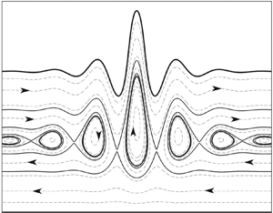
Figure 11 shows numerical results of particle trajectories of a downstream wave in figure 11(a) and of an upstream wave in figure 11(b) in the moving frame. Two different patterns, periodic transport trajectories and closed loops, are both found. However, the figure illustrates the difference in the location of closed orbits between downstream and upstream waves. If we consider waves in the laboratory frame, this phenomenon actually indicates that, when  $\varOmega$ and
  $c$ are of the same sign, the wave carries fluid particles beneath its crests, while, on the other hand, the upstream wave moves forward with fluid particles near the bottom. It is remarked that the frequency of the particle motion in the periodic transport regime is not uniform due to the shear current, which provides a non-uniform velocity distribution over water depth.

Figure 11.  $(a)$ Particle trajectories of a downstream wave with parameters
  $c=0.35$,
  $h=1$,
  $\lambda =2{\rm \pi}$ and
  $\varOmega =2$ in the moving frame. The uppermost curve is the displacement of the free surface, and both periodic transport trajectory and closed orbit are shown beneath it. Calculations are done in the time interval
  $[0,\lambda /c]$ and stars represent initial positions.
  $(b)$ Particle trajectories of an upstream wave for
  $t\in [0,3\lambda /c]$ with parameters
  $c=-5.65$,
  $h=5$,
  $\lambda =20{\rm \pi}$ and
  $\varOmega =1$ in the moving frame.
4. Solitary waves
The existence and stability of hydroelastic solitary waves propagating on a linear sheared current were investigated by Gao et al. (Reference Gao, Wang and Milewski2019). Solitary waves were computed numerically and envelope equations near to and away from resonance were derived to assist stability analyses. We follow their numerical techniques, and focus on the flow structure beneath solitary waves. The algebraic decay of hydroelastic solitary waves usually requires a long computational domain with a large number of grid points. Long periodic waves with flat tails are usually considered to be a good approximation of solitary waves. Here we take  $\lambda =200$ as the domain side, and 4096 Fourier modes are used in most of the computations to achieve a sufficient accuracy.
Two fundamental branches of symmetric solitary waves, including one family of waves with a positive free-surface elevation at the centre (denoted waves of elevation) and the other family of waves with a negative free-surface elevation at the centre (denoted waves of depression) are shown in figure 12 for downstream waves and in figure 13 for upstream waves. All the branches presented bifurcate from the minimum of the phase speed shown by a vertical dashed line where the group velocity is equal to the phase velocity. The interested reader is referred to Gao et al. (Reference Gao, Wang and Milewski2019) for more details on the bifurcation mechanism and its connection to the nonlinear Schrödinger equation. It is noteworthy that a smooth transition between upstream and downstream solitary waves along the same bifurcation curve is possible as the wave speed passes through zero (see figure 12a). Typical wave profiles are found to be similar to other wavepacket-type solitary waves (e.g. gravity–capillary waves in deep water). Hydroelastic solitary waves with constant vorticity are also characterised by oscillatory decaying tails.

Figure 12. Speed–amplitude bifurcation diagrams of hydroelastic solitary waves for  $\varOmega =1$ and
  $h=5$, together with typical wave profiles:
  $(a)$ elevation branch and
  $(b)$ depression branch. Waves corresponding to circles are plotted in the physical space, and the bifurcation point (
 $c=0.7652$) is shown by a dashed vertical line.

Figure 13. Speed–amplitude bifurcation diagrams and typical wave profiles of hydroelastic solitary waves in upstream flows:  $(a)$ elevation branch with
  $\varOmega =3$ and
  $h=2$ bifurcates from
  $c=-3.195$;
  $(b)$ depression branch with
  $\varOmega =3$ and
  $h=3$ bifurcates from
  $c=-3.215$. Wave profiles corresponding to circles are plotted in the physical space, and bifurcation points are shown by dashed vertical lines.
For hydroelastic solitary waves propagating against a non-uniform flow, particle trajectories show interesting patterns in the frame of reference moving with the wave, the most notable being the net displacement in the vertical direction indicating that the interaction between a solitary wave and a linear shear current can result in vertical mass transport (see figure 14). This is not observed in periodic waves. We take the particle on the left of the wave which experiences a net vertical displacement as an example. First the particle is chased by the solitary wave and swept downwards. Because the shear velocity increases with the water depth, the particle moves faster in deeper water and finally leaves the solitary wave far behind. It is worth noting that particles can also be swept upwards and never catch up with the solitary wave. In addition, figure 14 shows two other possibilities of particle trajectory patterns: closed orbits and pure horizontal transport. We remark that the calculations are carried out for large time periods.

Figure 14. Typical particle trajectories in an upstream elevation solitary wave with  $h=2$,
  $\varOmega =3$ and
  $c=-2.95$. The uppermost curve without a circle is the free-surface displacement, while the others represent particle trajectories with different starting points denoted by circles. Three trajectory patterns are observed in the frame of reference moving with the surface wave: closed orbit, pure horizontal transport, and net vertical displacement.
For a better understanding of the structure of the flow field, we plot a set of streamlines which represent different particle paths in a time-independent system. We show the flow structure resulting from an upstream elevation solitary wave in figure 15(a) with parameters  $c=-2.95$,
  $h=2$ and
  $\varOmega =3$. Only the active part of the horizontal domain near the main pulse is shown for better visibility. It turns out that, in the moving frame, the flow field can be divided into three layers in which streamlines and the dynamic behaviours of fluid particles are significantly different. For convenience, thick solid lines are used to show important streamlines separating different areas, while other streamlines are plotted as dashed curves.

Figure 15. Classification of streamlines under solitary waves with constant vorticity in the moving frame. Thick solid lines represent boundaries between different regions. Closed orbits and vertical-transport trajectories are intertwined and eventually form complex cat's-eye structures.  $(a)$ Streamlines beneath an upstream elevation solitary wave with
  $c=-2.95$,
  $h=2$ and
  $\varOmega =3$.
  $(b)$ Streamlines beneath an upstream depression solitary wave with
  $c=-3.03$,
  $h=3$ and
  $\varOmega =3$.
In the layer between curve A and the free surface, particles overall keep moving from left to right and oscillate when they are swept by the solitary wave, and the path profile is in general qualitatively similar to the wave profile. In the region between curve B and the bottom, particles are less affected by the free surface and move from right to left due to the large horizontal speed of the shear current. In the region between curve A and curve B, particles can either move along closed orbits or move vertically when they are swept by the solitary wave but finally move in the opposite horizontal direction. Under each crest of surface oscillations, there is a family of closed trajectories which is bounded by another family of vertical-transport curves and eventually form a series of cat's-eyes nested from large to small. These families of closed orbits are located in a fluid layer where the shear speed is nearly equal to the wave speed, and the cat's-eye structure gradually shrinks when it stays away from the middle pulse of the solitary wave.
Similar structures and trajectories can also be found in depression solitary waves, and a typical example is shown in figure 15(b) with parameters  $c=-3.03$,
  $h=3$ and
  $\varOmega =3$. It is remarked that closed streamlines were also computed in weakly nonlinear models for rotational gravity waves at much lower computational costs (see, for example, the numerical studies on the Benjamin equation by Segal et al. (Reference Segal, Moldabayev, Kalisch and Deconinck2017)). However,richer flow structures, such as nested cat's-eyes, can be expected in the fully nonlinear equations and beneath complicated wave profiles.
In the subsequent analyses, we explore the conditions under which the vertical-transport layer exists. Since there is no wave in the far field, the shear velocity should coincide with the wave speed in the horizontal centreline of the vertical-transport layer. It follows that the existence of vertical-transport zones requires a critical depth  $h_c$ such that
  $-\varOmega h_c=c$. This condition is twofold: For positive
  $\varOmega$,
  $c$ should be negative and no vertical-transport zone exists if
  $c<-\varOmega h$, which provides the two boundaries shown in figure 16, namely
  $c=0$ and
  $c=-\varOmega h$ (dashed lines). On the other hand, for fixed
  $\varOmega$ and
  $h$, there exists
  $c_{min}<0$ such that hydroelastic solitary waves of the wavepacket type can exist only for
  $c>c_{min}$, which gives another boundary shown as solid lines in figure 16 for different values of
  $h$. In the
  $\varOmega$–
 $c$ plane for fixed
  $h$, these boundaries form a semi-infinite region where vertical-transport zones exist (namely the right-hand side of the solid/dashed curve shown in figure 16).

Figure 16. Parameter region for the existence of a vertical-transport layer. The boundary of the region is composed of  $c=0$,
  $c=-\varOmega h$ (dashed line) and
  $c_{min}$ (solid line). The regions are shown in the
  $\varOmega$–
 $c$ plane for
  $h=1,2,5$, and vertical-transport layers exist only on the right-hand side of the solid/dashed line. Flow structures according to the black dot and asterisk in the inset are shown in figure 18(a) and (b), respectively.
Figures 17–19 show how the vertical-transport layer varies when the parameter set approaches each boundary for  $h=5$. Since
  $h_c$ decreases along with the absolute value of
  $c$, the vertical-transport layer moves upwards. It is observed in figure 17(a) that the layer of right-going trajectories first disappears, and the closer
  $c$ is to zero, the thinner the vertical-transport layer becomes (compare figure 17a and 17b). It turns out that the vertical-transport layer totally vanishes as
  $c$ becomes zero. Figure 18 compares the flow structures between two parameter sets sitting on both sides of the dashed line, which correspond to the black dot and asterisk in the inset of figure 16. As
  $h_c$ increases, the vertical-transport layer moves towards the bottom (figure 18a) and completely disappears when
  $h_c$ exceeds the upper bound
  $h$ (figure 18b). Finally, figure 19 shows the trend of the vertical-transport layer as the amplitude of the solitary wave decreases (or, equivalently,
  $c$ approaches
  $c_{min}$). The layer stays in the middle since
  $h_c\approx -\varOmega /c_{min}$, while the thickness of the layer narrows as the surface wave decreases from 0.2 to 0.08 in amplitude. Whether the middle layer will completely disappear depends on the bifurcation mechanism of hydroelastic solitary waves. More precisely, if the associated nonlinear Schrödinger equation is of focusing type at
  $c_{min}$, indicating that hydroelastic solitary waves bifurcate from infinitesimal periodic waves (Gao et al. Reference Gao, Wang and Milewski2019), then the vertical-transport layer will vanish as the wave speed reaches
  $c_{min}$, but not vice versa.

Figure 17. Streamline patterns beneath upstream hydroelastic solitary waves in the moving frame. Two distinct layers are observed.  $(a)$ Flow structure in an elevation wave with
  $\varOmega =1$,
  $h=5$ and
  $c=-0.37$.
  $(b)$ Flow structure in a depression wave with
  $\varOmega =1$,
  $h=5$ and
  $c=-0.01$.

Figure 18. Streamline patterns beneath upstream hydroelastic solitary waves in the moving frame.  $(a)$ The nested cat's-eye structure is observed at the bottom with
  $\varOmega =0.31$,
  $h=5$ and
  $c=-1.51$.
  $(b)$ Flow structure with
  $\varOmega =0.29$,
  $h=5$ and
  $c=-1.49$.

Figure 19. Vertical-transport layer beneath upstream depression solitary waves in the moving frame for  $h=5$ and
  $\varOmega =2$, with:
  $(a)$
$(a)$  $\eta (0)=-0.2$,
  $c=-2.6267$; and
  $(b)$
$(b)$  $\eta (0)=-0.08$,
  $c=-2.6361$. The zone shrinks as the amplitude of the free surface decreases.
5. Concluding remarks
In this paper the Stokes expansion up to third order has been carried out for flexural–gravity waves with a constant vorticity so that the nonlinearity manifests itself not only in the generation of higher-order harmonics but also in the correction of translating speeds. The full Euler equations were solved numerically using a conformal mapping technique, and travelling wave solutions, including periodic waves, bright solitary waves and generalised solitary waves, were computed. The Stokes expansion was used to validate the numerical algorithm by comparing periodic wave profiles, as well as particle trajectories, and very good agreements were found.
Further numerical calculations for the fully nonlinear equations focused on three topics: global bifurcation mechanisms of periodic waves, the existence of wave fronts, and flow structures beneath solitary waves. For upstream periodic waves, we showed that the global bifurcation includes a curve joining two infinitesimal periodic waves of different phase speeds, and a curve starting from an infinitesimal periodic wave and ending with a stationary state ( $c=0$). For downstream waves, the key finding of the broadening of the middle table-top structure of generalised solitary waves strongly suggests the existence of wave fronts characterised in the far field by a uniform state on one side and a train of waves on the other. To the best of the authors’ knowledge, it is the first example of wave fronts discovered in the full Euler equations in single-layer fluid problems. For particle trajectories beneath solitary waves, in the frame of reference moving with the wave, three patterns, including pure horizontal transport, net vertical displacement and closed orbit, are possible due to wave–current interactions. For upstream waves, a nested cat's-eye structure of streamlines was observed for both elevation and depression solitary waves.
Our numerical results raise further questions. A natural question is whether or not there are other global bifurcation mechanisms. On the theoretical side, the global bifurcation of pure gravity waves with arbitrary vorticity was initially investigated by Constantin & Strauss (Reference Constantin and Strauss2004). They showed three bifurcation mechanisms. Apart from two cases presented in § 3.3, an unbounded bifurcation is also a possibility. Akers et al. (Reference Akers, Ambrose, Pond and Wright2016) and Akers et al. (Reference Akers, Ambrose and Sulon2017) investigated the global bifurcation of interfacial capillary–gravity waves and interfacial hydroelastic waves, respectively, using analytical and numerical tools. They provided some numerical evidence for the existence of unbounded bifurcation curves on which the wave amplitude increases without limit. Therefore, one can ask whether or not there are unbounded branches of hydroelastic periodic waves propagating on a linear shear current.
The discovery of wave fronts also introduces questions. Since all the wave-front solutions were found in downstream waves in the present paper, a first question is if we can also find wave fronts for upstream waves. With respect to the asymptotic models for this phenomenon, the fifth-order KdV equation with non-convex dispersion, which admits TDSWs (Sprenger & Hoefer Reference Sprenger and Hoefer2017), is a reduced model for flexural–gravity waves in the shallow-water regime for potential flows (Xia & Shen Reference Xia and Shen2002). Therefore, it is also expected to be an appropriate model in the presence of a linear shear current so as to explain the wave-front phenomenon found in this paper. A comparative study of wave-front solutions between the asymptotic model and the primitive equations, as well as numerical simulations of the generalised Riemann problem for the full Euler equations, will be reported elsewhere in the near future. Another direction of extension related to TDSWs is to generalise the Whitham modulation equations (see Whitham (Reference Whitham1974) for details) to waves with vorticity. In order to use Whitham's argument for slowly varying wave trains, the Lagrangian formulation of the problem is a prerequisite. Therefore, it is of great interest to find an explicit Lagrangian density for unsteady water waves with vorticity and extend Whitham's ‘averaged variational principle’ to these waves.
Acknowledgements
Z.W. would like to thank Dr E. Vărvărucă (University Alexandru Ioan Cuza) for helpful discussions on matters relating to this article. Z.W. and X.G. were supported by the National Natural Science Foundation of China (no. 11772341), the Key Research Program of Frontier Sciences of CAS (no. QYZDBSSW-SYS015), and the Strategic Priority Research Program of the Chinese Academy of Sciences (no. XDB22040203). They would also like to acknowledge the support from CAS Center for Excellence in Complex System Mechanics. J.M.V.-B. was supported in part by EPSRC under grant EP/N018559/1.
Declaration of interests
The authors report no conflict of interest.


