


1. INTRODUCTION
For a high power megawatt class accelerator, any loss, even a tiny proportion of the beam, can be harmful. Classical beam manipulating precautions or usual protection systems may not be sufficient. A careful and detailed loss study is thus necessary for various loss scenarios. Beam dynamics simulations should be performed in order to provide a most exhaustive possible catalogue of losses, where the power and the location of possible losses should be estimated at least along the high power part. That should be analyzed for all the different stages of the accelerator lifetime, from its starting up, beam commissioning through routine operation, as well as for the various accidental breakdowns.
Such a catalogue will be useful, or even necessary in the definition of safety procedure, limitations and recommendations, aiming at protecting personnel or facilities. The resulting losses should be finally considered for example when: (1) designing the PPS or personal or machine protection system; (2) setting the maximum authorized beam power and/or test duration for beam commissioning or tuning; (3) setting the maximum authorized field variation range in the control system; (4) identifying the hot points deserving further protection.
In this article, the case of the Linear IFMIF Prototype Accelerator (LIPAc) is studied. This accelerator is being constructed in Europe and installed in Japan (Mosnier et al., 2010). The general layout of LIPAc is recalled in Figure 1, where beam energy and power for each subsystem are also given (for more details see, Nghiem et al., Reference Nghiem, Chauvin, Comunian, Delferrière, Duperrier, Mosnier, Oliver and Uriot2009a; Reference Nghiem, Chauvin, Comunian, Delferrière, Duperrier, Mosnier, Oliver, Simeoni and Uriot2011; Reference Nghiem, Chauvin, Comunian, Delferrière, Duperrier, Mosnier, Oliver and Uriot2014; Chauvin et al., Reference Chauvin, Delferrière, Duperrier, Gobin, Nghiem and Uriot2009a; Reference Chauvin, Duperrier, Mosnier, Nghiem and Uriot2009b; Reference Chauvin, Delferrière, Duperrier, Gobin, Mosnier, Nghiem and Uriot2011; Reference Chauvin, Delferrière, Duperrier, Gobin, Nghiem and Uriot2012; Comunian & Pisent, Reference Comunian and Pisent2011; Delferrière et al., Reference Delferrière, Tuske, De Menezes, Harrault and Gobin2007; Oliver et al., Reference Oliver, Brañas, Ibarra, Podadera, Chauvin, Mosnier, Nghiem and Uriot2008). The 125 mA continuous wave D+ beam is extracted from the ion source then transported and accelerated successively through a LEBT with two solenoids, a long RFQ, a MEBT with five quadrupoles and two bunchers, a superconducting radio-frequency (SRF) Linac with eight solenoids and eight accelerating cavities, a HEBT with one dipole and eight quadrupoles, to hit finally a beam dump. All the simulations in this article have been made in this configuration.

Fig. 1. (Color online) Layouts of the IFMIF prototype accelerator.
The LIPAc very high continuous wave beam intensity implies that almost the whole accelerator is concerned by a high power beam which ranges from 0.012 to 1.125 MW. Under these conditions, the usual precautions or protections become questionable. Indeed, it is common to consider that it is safe enough to use the lowest duty cycle and the lowest beam intensity during beam commissioning or exploration. But in the present case, as the ion source is optimized for providing a continuous beam, the lowest duty cycle for which the beam is still stable is 10−3; furthermore, the nominal beam intensity implies a very high space charge regime so that any beam tuning with too low intensity will not be representative because of much lower space charge effects. Thus, the ability to lower the beam power is considerably limited. In the same way, a beam stop system is foreseen in the LEBT to shut off the beam in an accidental case in less than 10 µs as usual. But it is not sure that it is fast enough for a MW beam power.
In the following, after important preliminary remarks explaining how to interpret the results shown in this article, the protocol of loss simulations is discussed, then the loss results are given in the different loss scenarios and for each of them the consequences on safety measures are drawn.
2. PREAMBLE
It is important to notice the following statements before using the results of this article. The losses are given here in power deposition (Watt). They are obtained with the nominal (maximum) current of 125 mA continuous wave. From that, losses can be reduced if needed, by reducing consequently the duty cycle and even the current if necessary. Theoretically, because space charge effects decrease with intensity, losses at lower current are less than what can be inferred by a linear relation. But as a precaution, it is wise to deduce losses at lower current with a simple linear transformation. Always as a precaution, a comfortable margin (a factor 2 to 10, for example) should be added to the loss values given by the present studies, before any consideration at safety level.
3. LOSS STUDY PROTOCOL
The double issue is to define as exhaustively as possible all the typical loss situations in the accelerator lifetime and to define the procedure to simulate and estimate them. A protocol for studying losses has been discussed within the beam dynamics group for several years and was first reported in Nghiem et al. (Reference Nghiem, Chauvin, Comunian, Delferrière, Duperrier, Oliver and Uriot2009b; Reference Nghiem, Chauvin, Comunian, Delferrière, Duperrier, Mosnier, Oliver, Simeoni and Uriot2011; Reference Nghiem, Chauvin, Comunian, Oliver and Uriot2012). Since then, it has again been discussed and updated many times. It appears that studies according to the situations and the protocols described in the following should be enough for characterizing losses in all the stages of the accelerator lifetime (See Table 1): (1) Ideal machine; (2) Starting from scratch; (3) Beam commissioning, tuning, exploration; (4) Routine operation; (5) Sudden failure.
Table 1. Loss study simulations and results for the different possible situations (the number of 500 start-to-end simulations is a compromise between a good statistic result and the computation time)

3.1. Ideal Machine
“Ideal” means here nominal theoretical conditions, without any error. That should correspond on the real machine to a completely satisfying situation, once all the technical components are perfectly fabricated and aligned, or else perfectly corrected at the source, and the beam has been perfectly tuned. Losses in such conditions should be minimum; we cannot hope to have less. These are minimum and permanent losses that have to be withstood. They are obtained by a start-to-end simulation without any error for the nominal tuning.
3.2. Starting From Scratch
In this condition, no correction has yet been applied, while we can expect that: (1) The technical components have been fabricated and aligned as specified, within the already defined tolerance ranges. (2) The tunable parameters (fields and gradients) are set at their nominal theoretical values. We must however expect that the real beam behavior is not exactly the same as theoretically simulated (the IFMIF very high space charge regime has never been experimentally observed). This theory-reality difference can be roughly estimated as equivalent to field and gradient variations in a ±10% range of their nominal values, according to the beam dynamics optimization results obtained in different working configurations since the beginning of the project.
Losses when starting from scratch can thus be estimated by performing 500 start-to-end simulations without any correction in the presence of random “errors” of two kinds: mechanical, alignment errors randomly distributed within tolerances and tunable parameter errors (gradients, fields) randomly distributed within a ±10% range of their nominal values. Tolerance values, including static and dynamic ones, are discussed and presented in Chauvin et al. (Reference Chauvin, Delferrière, Duperrier, Gobin, Mosnier, Nghiem and Uriot2011) and Nghiem et al. (Reference Nghiem, Chauvin, Comunian, Delferrière, Duperrier, Mosnier, Oliver, Simeoni and Uriot2011; Reference Nghiem, Chauvin, Comunian, Delferrière, Duperrier, Mosnier, Oliver and Uriot2014). Losses for each location along the accelerator are then collected for all the simulated cases, from which curves of loss probability can finally be deduced.
3.3. Beam Commissioning, Tuning, Exploration
This occurs during beam commissioning or whenever the beam operation is not as satisfying as theoretically expected so that a beam tuning is necessary, or else when an exploration around a nominal setting is desirable. Those situations take place at different epochs of the accelerator life. However, the induced beam losses can be calculated in the same way. As in the previous case 3.2, we can assume mechanical errors within tolerances and tunable parameter variations of about ±10%. The only difference is that now the trajectory is corrected. Losses can thus be quantified by the same simulations as in case 3.2, but with trajectory correction.
3.4. Routine Operation
This can be performed when the beam characteristics are satisfying, i.e., as theoretically expected with all the parameters, mechanical and tunable parameters, as specified within tolerances and the trajectory corrected. Losses can thus be calculated by performing 500 start-to-end simulations with all the errors within tolerances, in the presence of trajectory correction.
3.5. Sudden Failure
These accidental situations are not easy to be exhaustively studied, especially when a combination of different failures can lead to more important losses than an individual failure. Reflexions and analysis should be carried out for each subsystem to detect what is the worst case, what is the main affected location or equipment, when one tunable parameter (gradient, field, phase, RF power, pressure …), or a given combination of them, are suddenly switched off. But attention should also be paid to detect if there is an intermediate case which can induce more losses, for example, in the transition from the nominal value to zero for specific field or gradient. In this article, only two cases are studied: failure of individual components and global failure of all the components at once, from 110% to 0% of their nominal values. This can be due to power supply failures that accidentally provide a larger power or that can be suddenly switched off, making the fields or gradients returning progressively to zero.
4. BEAM LOSSES FOR AN IDEAL MACHINE
Start-to-end simulations with 106 macro-particles have been thoroughly carried out with the TraceWin code (Duperrier et al., Reference Duperrier, Pichoff and Uriot2002). The used input beam results from calculations of the ECR source extraction system with the AXEL code (Spädtke, Reference Spädtke2008), and most of the elements of the accelerators are represented by their field map calculated by finite element methods.
Losses in the nominal case are given in Figure 2. Losses occur in the first part of the RFQ (1 kW integrated), in the MEBT where scrapers have been installed to collect them (10 W) and in the bending magnet (1 W). They all come from particles not correctly bunched and accelerated by the accelerating structures which are the RFQ and the SRF-Linac. For more details, see Chauvin et al. (Reference Chauvin, Delferrière, Duperrier, Gobin, Mosnier, Nghiem and Uriot2011) and Nghiem et al. (Reference Nghiem, Chauvin, Comunian, Delferrière, Duperrier, Mosnier, Oliver and Uriot2014).

Fig. 2. (Color online) Beam power lost for the ideal machine.
5. BEAM LOSSES WHEN STARTING FROM SCRATCH
This situation is, with certain accidental situations, among those where losses are the most important. As specified in the previous sections, loss probabilities are calculated according to 500 start-to-end simulations with mechanical errors randomly distributed within tolerances and tunable parameter (field, gradients) errors randomly distributed within ±10% of their nominal values.
Notice that no correction is applied. The cavity phases and the RFQ voltage are not considered here as tunable parameters. They are left at their nominal values. The dipole field is not a tunable parameter like the other one, its variation should be much less. We have chosen the ±3% variation range for it (to be compared to the ±1% tolerance). Simulations are performed for the nominal 125 mA continuous wave beam current. Once losses are known, a proportional calculation will give the maximum acceptable duty cycle or current at starting to avoid harmful losses. Loss probabilities along LIPAc are given in Figure 3.

Fig. 3. (Color online) Beam power loss probabilities when starting from scratch for a full-power beam (statistics over 500 machines). The bottom figure is a zoom of the top one.
Losses are the smallest in the low-energy part, because only two tunable elements are implied, the two solenoids. The maximum peaks are about 1000 W in the LEBT and 100 W in the RFQ. If only this part is started from scratch, 10−3, 10−2 of beam nominal power would be fine.
Losses are huge in the high-energy part. That could be pessimistic because generally this part is started after the low energy part was already correctly tuned, which is not simulated here by the start-to-end simulations. However, it is not too pessimistic because losses due to the low-energy part are very weak compared to those due the high-energy one. Losses occur mainly at the fixed scraper in front of the beam dump and in the solenoids of the cryomodule, or more precisely at their exits where the beam stay clear is abruptly reduced. Less but noticeable losses can be seen in the quadrupoles surrounding the dipole and also within the dipole and the diagnostic plate. The maximum peaks, corresponding to 0.2% of the simulations, reach hundreds of kW. In 5% of the simulations, losses still go up to 300 kW at the beam dump scraper and 70 kW locally in the cryomodule, with an integrated power of about 200 kW. It can be recommended to take these last numbers into consideration because 5% of the simulations mean 25 over the 500 studied cases, a small but not negligible chance. As no more than about 10 W of heat deposited by the particle beam can be drained away by the cryogenic system, only 10−6, 10−5 of nominal beam power can be accepted when starting the accelerator from scratch. Considering that the beam quality (stability and representativeness as discussed in Section 1) becomes questionable at a duty cycle down to 10−3 or a beam current down to 100 mA, the implementation of a high-performance chopper in the LEBT is absolutely crucial, with a rise time better than 1 µs. The availability of beam diagnostics for such a low beam power should also be assessed.
6. BEAM LOSSES DURING BEAM COMMISSIONING, TUNING OR EXPLORATION
Beam commissioning on one hand and beam tuning or exploration on the other hand, take place at different times of the accelerator life. However, as discussed in Section 3, beam losses in these different situations can be calculated in the same way, with 500 simulations in exactly the same conditions as in section 5, except that now the trajectory is corrected. Loss probabilities along LIPAc are given in Figure 4.

Fig. 4. (Color online) Beam power loss probabilities during beam commissioning, tuning or exploration, for a full-power beam (statistics over 500 machines). The bottom figure is a zoom of the top one toward the low power losses.
Compared to the case without trajectory correction, losses do not change much in the low-energy part, because the trajectory deviation was not important in this part. The maximum peaks are 1000 W in the LEBT and slightly less than 100 W in the RFQ. Particles that are not lost and can now exit the RFQ are intercepted by the MEBT scrapers (movable, but here left fixed at its nominal position) (see, Nghiem et al., Reference Nghiem, Chauvin, Comunian, Delferrière, Duperrier, Mosnier, Oliver, Simeoni and Uriot2011) where maximum losses increase up to hundreds of W.
Losses in the fixed beam dump scraper are slightly bigger compared to the case without correction. That means that these losses mainly come from the trajectory deviation due to dipole field variations, which is not corrected in the present studies. In reality, continuous trajectory correction while varying the dipole field would well decrease these losses.
Only maximum losses in the cryomodule, at the solenoid exits, have decreased by a factor of 2, while losses in 5% of the simulations still remain to be 70 kW locally with an integrated power loss of more than 100 kW. In the meantime, losses downstream within the diagnostic plate, the dipole and the quadrupole surrounding the dipole have increased, reaching tens of kW.
In these conditions, only 10−5 of nominal beam power can be accepted considering that no more than about 10 W of heat deposited can be accepted by the cryogenic system. A high-performance chopper with a rise time better than 1 µs is thus absolutely needed in the LEBT, as the source is no longer stable at a duty cycle lower than 10−3 and beam intensity lower than 100 mA is not representative because of its much lower space charge regime.
In case of beam tuning or exploration, it can also be recommended to proceed by maximum variations at once of 5% of the nominal values and not 10% as in the present studies. This maximum authorized variation per step should be introduced into the accelerator control system.
7. BEAM LOSSES DURING ROUTINE OPERATIONS
As discussed in Section 3, beam losses during routine operations are calculated according to 500 start-to-end simulations with all the errors, mechanical and tunable parameters, randomly distributed within tolerances, with trajectory corrected. This is a little pessimistic because in reality the tunable errors can be well better compensated. Loss probabilities along LIPAc are given in Figure 5.

Fig. 5. (Color online) Beam power lost probabilities in case of routine operation (statistics over 500 machines).
Compared to the ideal machine without any error, the loss locations are similar, i.e., mainly within the RFQ. Losses are here about a factor of 2 higher, 16 W locally, about 2 kW integrated, while elsewhere there is less than 1 W, except at the dipole exit and the beam dump scraper where there are a few W. This demonstrates that the accelerator can be operated at the specified 125 mA in continuous mode. Notice that these results have been already obtained in an earlier stage (Chauvin et al., Reference Chauvin, Delferrière, Duperrier, Gobin, Mosnier, Nghiem and Uriot2011; Nghiem et al., Reference Nghiem, Chauvin, Comunian, Delferrière, Duperrier, Mosnier, Oliver and Uriot2014), based on which the error tolerances have been set.
8. BEAM LOSSES IN CASE OF SUDDEN FAILURE
As discussed in Section 3, beam losses in case of sudden failure will be calculated only for two configurations: (1) Individual elements at 110% to 0% of their nominal values. As for example a sudden failure of a quadrupole or a cavity power supply, inducing a higher field, up to 110% or its sudden breakdown so that it collapses progressively from 100% to 95, 90, 85, 80, 75, 50, 25, 0%. (2) All the elements at 110% to 0% of their nominal values, as for example in case of dysfunction or sudden electricity breakdown of the whole accelerator site.
Failure of steerers are not included because the induced losses are completely negligible compared to those induced by any other element.
Due to the number of different components and their nature which are very different in the low-energy part (until the end of the RFQ, E ≤ 5 MeV) and the high-energy part (from the MEBT, E≥ 5 MeV), the loss studies are performed separately for each of them.
8.1. Sudden Failures in the Low-Energy Part
Beam loss powers are given in Figures 6, 7, and 8 for the cases of sudden failure of the first LEBT solenoid, then the second solenoid, then the RFQ. The case of global failure of all the elements at once is given in Figure 9.

Fig. 6. (Color online) Beam lost power in case of sudden failure of the first LEBT solenoid.

Fig. 7. (Color online) Beam lost power in case of sudden failure of the second LEBT solenoid.

Fig. 8. (Color online) Beam lost power in case of sudden failure of the RFQ.

Fig. 9. (Color online) Beam lost power in case of sudden failure of the low-energy part at once.
Failures of the first solenoid induce losses mainly at the RFQ entrance cone, of several kW, when its field is only at ± 4% of its nominal value. However, according to transmission measurements and simulations during the injector beam commissioning, a ± 5% margin could be expected (Chauvin et al., Reference Chauvin2013). As a consequence, the emergency beam stop system should be able to stop the beam before the first solenoid field varies outside the 95–105% range. Anyway, the RFQ entrance cone area is clearly a hot point that must be protected and cooled down so that at least 5 kW beam losses can be withstood.
Failures of the second solenoid generate much less losses at the RFQ entrance, of about 100 W, until 80% of its nominal value where losses again reach several kW. That is because its field is much smaller than that of the first solenoid, being nevertheless necessary for beam focusing.
The RFQ voltage induces more losses only when it decreases. In case of sudden breakdown, losses of a few W locally within the RFQ are not worrying until 95% of its nominal value. As soon as the voltage decreases to 90%, losses of about 10 W appear at several solenoids in the cryomodule, and about 100 W at the dipole exit. These losses are multiplied by 10 when the voltage decreases to 85%. To preserve the solenoids and the dipole exit areas, it is therefore important to be able to stop the beam not later than when the RFQ voltage reaches 95% its nominal value.
When all the low-energy part suddenly failed, the three loss mechanisms described above are combined, making that losses at the RFQ entrance are slightly bigger, implying up to almost the whole beam, and consequently decreasing strongly losses downstream the RFQ. This case is thus less harmful than that of RFQ failure alone for the sections downstream the RFQ.
8.2. Sudden Failures in the High-Energy Part
As previously, two cases of failure have been thoroughly studied: failure of each element individually while all other ones stay at their nominal setting and global failure of all the focusing elements at once. Failures mean accidental trip to a higher value or going to zero by passing through intermediate values. Simulations have been performed for field and gradient strengths at 0, 25, 50, 75, 80, 85, 90, 95, 105, and 110% of their nominal value, which is referred as 100%.
For the high-energy part (E ≥ 5 MeV), from the MEBT to the beam dump, many different elements are used for focusing or accelerating the beam: quadrupoles, solenoids, bunchers, accelerating cavities, and dipole. Simulations of individual failure for each of them, though tedious, are nevertheless (bravely!) done. However, presentations of losses along the accelerator induced by each element failure are not convenient. That is why, only the maximum losses (among losses due to the different individual failures) for each position z are reported in Figure 10. It is worth mentioning that even in case of small losses, the field trips can induce important beam size variations that the beam dump cannot withstand. These variations have also been carefully studied in Figure 11. Losses in case of global failure of all the elements of the high-energy part at once are given in Figure 12, and the resulting beam size variations in Figure 13.

Fig. 10. (Color online) Maximum beam losses in case of sudden failure of individual elements in the high-energy part (the dipole failure is not included).
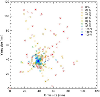
Fig. 11. (Color online) Beam r.m.s. size at the beam dump entrance in case of sudden failure of the individual elements of the high-energy part (the dipole failure is not included). The dashed circle represents the tolerated beam size variation at the beam dump entrance.

Fig. 12. (Color online) Beam losses induced by sudden failure of all the elements in the high-energy part at once (the dipole failure is not included).

Fig. 13. (Color online) Beam r.m.s. size in case of sudden failure of all the elements of the high-energy part at once (the dipole failure is not included). The dashed circle represents the tolerated beam size variation at the beam dump entrance.
We can observe that losses induced by individual element breakdowns are generally higher by a factor of 2 compared to a global breakdown of all elements. That is due to the focusing-defocusing quadrupoles that must be used in combination. Failures around 85–110% imply losses on the order of hundreds W, while higher failures imply losses up to hundreds of kW. On the other hand, as a variation of only ±10 mm around the nominal r.m.s. beam radius can be tolerated, then only field trips less than 95–105% can be authorized. (Note that an important asymmetrical beam size at the beam dump can correspond to a very low current because strong losses occurred somewhere upstream. These cases are thus not specifically dangerous for the beam dump itself but are anyway dangerous for upstream equipment.)
The hot points can also be easily identified. They are different for the cases of global or individual failure. In case of global failure, the last HEBT drift is the most exposed for small field trips, while the MEBT last part and the SRF Linac first part is the most exposed for high field trips. In case of individual failure, the hottest regions are the second scraper, the fourth quadrupole in the MEBT, the 6th solenoid in the SRF Linac, the diagnostic plate, the last triplet and the scraper in the HEBT.
Notice that the dipole failure was not included in the above studies because of its particular behavior. Down to 85% of the nominal dipole field, no loss is generated. But at 80%, losses around the beam dump scraper reach hundreds of kW, and 70% the whole beam is lost.
Machine protection systems should be designed so that, in case of sudden failure, the beam is stopped the latest when the components in the high-energy part reaches 85% of their nominal values, or as early as 95% if in addition considerations of beam size at the beam dump must be taken into account.
9. CONCLUSIONS
Beam dynamics simulations have been performed in order to estimate beam losses during different stages of the LIPAc lifetime. That is meant to be a starting point for assessing all the accelerator safety aspects. That should concern all the accelerator subsystems by the identified hot points to be protected (facing beam equipment and diagnostics), the machine protection system by the requested beam stop velocity, the control system by the limitations to be imposed to power supply variations and the beam operations by the maximum beam power to be planned depending on each situation.
The main results are summarized as follows. The low-energy part refers to the section from the source to the end of the RFQ while the high-energy part stands for the section downstream until the beam dump. The nominal beam power refers to 125 mA beam intensity in continuous mode.
(1) Starting from scratch. The hot points are the RFQ entrance cone, the cryomodule solenoid exits, and the beam dump scraper. Starting the low-energy part with a 10−4, 10−3 nominal beam power would be fine. The high-energy part should be started with no more than 10−6, 10−5 of nominal beam power. Therefore, a high-performance beam chopper in the LEBT is absolutely needed (rise time < 1 µs).
(2) Beam commissioning or tuning or exploration. The same precautions as in the precedent case are necessary. In order to preserve the cryogenic section, no more than 10−5 of nominal beam power can be accepted, so that the role of a high-performance beam chopper in the LEBT is absolutely crucial. In case of tuning or exploration, variations of tunable parameters should be limited by the Control System to a maximum of 5% per step around a given setting.
(3) Routine operation. The loss locations are similar to those of the ideal machine, i.e. mainly within the RFQ. Here, losses are less than 20 W locally, about 2 kW integrated, while elsewhere there is less than 1 W, except at the dipole exit and the beam dump scraper where there are a few W. This theoretically demonstrates that the accelerator can be operated at the specified 125 mA continuous wave beam intensity.
(4) Sudden failure. Fields and gradients are supposed to suddenly increase from 100% to 110% or decrease to 0%. Failures of individual elements are generally more harmful than failure of all the elements at once. Not surprisingly, the hottest point is the RFQ entrance where the cooling system must be capable to remove at least 5 kW beam losses. The beam stop system must also be able to stop the beam whenever the first solenoid field varies outside the range 95–105% of its nominal value. In order to protect the superconducting elements, the most critical parameter to keep a close eye on is the RFQ voltage. The emergency beam stop system must stop the beam the latest when the RFQ voltage reaches 95% of its nominal value. For the elements of the high-energy part, the beam must be stopped when they reach 85% of their nominal value. Unless the Beam Dump can only accept variations of beam r.m.s. size less than ±10 mm, in which case the beam must be stopped for every element variation outside 95–105%.
The impact of those results on almost all the accelerator subsystems show the importance of setting up such a catalogue of losses for a high power accelerator or at least the high power part of an accelerator, where the beam power reaches more than hundreds of kW. The protocol of loss studies presented in this article can likely be applied to any accelerator, by appropriately adjusting the numerical values used here.


