


1. Introduction
In the low-disturbance environments typical of hypersonic flight (or most ground-test facilities), the path to boundary-layer transition on slender smooth bodies at small incidence is characterized by linear growth of instabilities within the boundary layer leading up to nonlinear modal interactions and breakdown (Fedorov Reference Fedorov2011), with the dominant instability for axisymmetric or near-axisymmetric geometries being the Mack or second mode (Mack Reference Mack1975). The outer mould line of a true flight vehicle does not always consist of smoothly varying surfaces, however, and may exhibit sudden changes in geometry, e.g. at a control surface or intake. In supersonic flow, such configurations result in shock wave–boundary layer interactions (SWBLIs). These SWBLIs can give rise to new instability mechanisms (particularly in the separated case – see e.g. Guiho, Alizard & Robinet (Reference Guiho, Alizard and Robinet2016), Roghelia et al. (Reference Roghelia, Olivier, Egorov and Chuvakhov2017) and Sidharth et al. (Reference Sidharth, Dwivedi, Candler and Nichols2018)), but would also be expected to affect disturbances propagating in from the upstream boundary layer, potentially leading to complex unsteady interactions.
Much of the prior work on two-dimensional (2-D) SWBLIs has sought to characterize transitional effects on flow topology (e.g. separation length and unsteadiness) and thermomechanical surface loading (Heffner, Chpoun & Lengrand Reference Heffner, Chpoun and Lengrand1993; Benay et al. Reference Benay, Chanetz, Mangin, Vandomme and Perraud2006; Running et al. Reference Running, Juliano, Jewell, Borg and Kimmel2018). Benitez et al. (Reference Benitez, Jewell, Schneider and Esquieu2020) employed focused laser differential interferometry (FLDI) to interrogate the separated boundary layer on a cone–cylinder–flare model. Low-frequency (50–170 kHz) travelling waves were identified downstream of the compression corner under quiet flow conditions, but could not be located within the separation region. Point-like measurement techniques like FLDI, however, necessarily preclude a global view of instability development.
Only a limited number of studies have elucidated transition dynamics or the impact of the SWBLI on pre-existing disturbances. For example, Balakumar, Zhao & Atkins (Reference Balakumar, Zhao and Atkins2005) used both linear stability theory (LST) and direct numerical simulation (DNS) to study 2-D fixed-frequency disturbances in a flat-plate boundary layer encountering a  $5.5^{\circ }$ compression corner at Mach 5.373. LST revealed the existence of multiple unstable modes within narrow regions of the separation bubble, while DNS showed the second-mode waves to be of neutral stability while traversing the separated shear layer but to grow exponentially upstream of separation and downstream of reattachment. Novikov, Egorov & Fedorov (Reference Novikov, Egorov and Fedorov2016) carried out DNS of three-dimensional broad-spectrum wavepackets on this same configuration. Both oblique-wave- and second-mode-dominated wavepackets were examined; the latter were found to be neutrally stable within the upstream part of the separation region before amplifying downstream. Strong forcing resulted in significant streamwise stretching of the wavepacket tail and the formation of a turbulent spot downstream of reattachment.
The objective of the present work is to improve our understanding of the interactions of hypersonic laminar boundary-layer disturbances – in particular, second-mode waves – with the mean flow structures introduced by a sudden change in surface angle. We focus on a compression-corner interaction with a modest ( $10^{\circ }$) angle change, sufficient to produce flow separation at the conditions examined but still within the range that one might expect to encounter on a practical hypersonic vehicle.
2. Experimental methodology
2.1. Facility overview
All experiments were performed in HyperTERP, a small-scale reflected shock tunnel operated by the University of Maryland. A contoured Mach 6 nozzle with a 22 cm exit diameter was employed, exhausting into a 30.5 cm diameter free-jet test section equipped with 15.2 cm diameter windows. A more detailed description of the facility is given in Butler & Laurence (Reference Butler and Laurence2019). The total specific enthalpy was held approximately constant at  $0.89\ \textrm {MJ}\ \textrm {kg}^{-1}$, with unit Reynolds numbers of
  $3.02\times 10^6$,
  $4.16\times 10^6$ and
  $4.94\times 10^6\ \textrm {m}^{-1}$ achieved by varying the reservoir pressure. Reservoir and corresponding free-stream properties for each condition are detailed in table 1. In all cases the steady test time is
  ${\sim }6\ \textrm {ms}$, during which the reservoir-pressure unsteadiness is typically 2 % (standard deviation). Shot-to-shot variation in the mean pressure is of the order of 1.3 %, while systematic uncertainty (combined calibration and nonlinearity) is estimated as 1.6 %. Shock-speed estimates are accurate to
  ${\pm }5\ \textrm {m}\ \textrm {s}^{-1}$, contributing 0.4 % uncertainty in the reservoir temperature. Also included in table 1 are estimated separation and reattachment locations, to be discussed shortly.
Table 1. HyperTERP test condition matrix, together with estimated separation and reattachment locations.

2.2. Test article and instrumentation
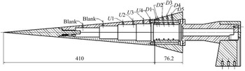
The bicone model that constituted the primary test article is pictured in figure 1; it consists of a 410 mm,  $5^{\circ }$ half-angle frustum and a 76.2 mm,
  $15^{\circ }$ half-angle flare. The nose radius was measured to be 0.10 mm using a SmartScope optical gauge. The short test duration in HyperTERP does not allow for significant model heating, meaning the wall temperature may be safely assumed to remain at approximately 300 K. Tests were also performed on a straight-cone configuration (
 $5^{\circ }$ half-angle flare) to provide comparisons against an undisturbed boundary layer.

Figure 1. Model schematic showing sensor layout (all dimensions in millimetres).
A single streamwise row of PCB 132B38 pressure transducers was installed along the upper surface of the cone as shown in figure 1, held in place using clear nail polish (Ort & Dosch Reference Ort and Dosch2019). These sensors were sampled at 2 MHz with a  $600\ {\rm kHz}$ low-pass filter to remove aliasing effects, though it should be noted that Ort & Dosch (Reference Ort and Dosch2019) observed resonances at frequencies above 300 kHz for this PCB model. Indeed, a 300 kHz peak was observed in many of the spectra in the present experiments (see figure 5) and results near this frequency should be treated with caution. These PCB sensors have previously been noted to be sensitive to structural excitation, and the impulsive loading inherent to flow start-up in shock tunnels may account in part for the large magnitude of these peaks.
2.3. Calibrated schlieren
High-speed flow-field visualization was obtained from a standard Z-type schlieren with a horizontal knife edge. Light pulses of  $20\ \textrm {ns}$ duration were provided by a Cavilux HF laser, and a Phantom v2512 camera was used to capture the images at 822 kHz, allowing resolution of spectral content up to 411 kHz. This frame rate was chosen to be significantly higher than the Nyquist sampling rate of the dominant second-mode frequencies. The field of view was
  $512\ \textrm {pixel} \times 32\ \textrm {pixel}$, with the camera rotated to maximize the region of flow visualized. A calibration procedure as described by Hargather & Settles (Reference Hargather and Settles2012) was used to convert the pixel intensities to integrated density gradients. Following the implementation of Kennedy et al. (Reference Kennedy, Laurence, Smith and Marineau2018), a plano-convex lens was placed into the field of view and a reference image captured; the intensity profile along the lens face was then mapped to the known density-gradient profile of the lens.
3. Results
3.1. General behaviour
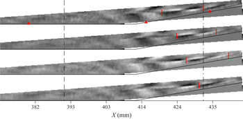
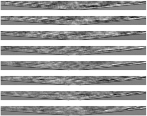
Time-resolved visualization sequences are presented in figures 2, 3 and 4, showing the development of second-mode wavepackets at each condition. The images have been rotated to align the abscissa with the frustum surface, with the  $X$ coordinate denoting distance along this frustum from the cone nose tip. Supplementary movies available at https://doi.org/10.1017/jfm.2021.91 are included online, showing the test-time sequence of raw images alongside reference-subtracted and bandpass-filtered versions for each test. At the top of each sequence is shown an average flow-on image to highlight the mean flow features; this has been subtracted from the subsequent time-resolved images in each sequence to emphasize transient features. The inter-image spacing in each case is
  $9.7\ \mathrm {\mu }\textrm {s}$. Red triangles denote the locations of (from left to right) PCB sensors
  $U3$,
$U3$,  $D1$ and
  $D3$. Red bars are used to bracket features of interest as they propagate along the cone surface. Power spectral densities (PSDs) for select PCB sensors are shown in figure 5 for each experiment. Approximate separation and reattachment locations are represented in each image sequence by vertical dashed lines, with corresponding numerical values provided in table 1. These locations were identified as points at which the pseudo-streamline profiles reported in § 3.2 exhibited a sudden change in slope; reasonable agreement was obtained between these results and preliminary numerical simulations. The uncertainty in each location is estimated as
  ${\pm }3\ \textrm {mm}$.

Figure 2. Reference-subtracted image sequence captured at condition Re30 with inter-image spacing of  $9.7\ \mathrm {\mu } \textrm {s}$.

Figure 3. Reference-subtracted image sequence captured at condition Re42.

Figure 4. Reference-subtracted image sequence captured at condition Re49.

Figure 5. Representative PSDs for select PCB stations at (a) condition Re30, (b) condition Re42 and (c) condition Re49.
The sequence of images in figure 2 depicts a single wavepacket traversing the separation region at condition Re30. In the PCB spectra for this condition, substantial growth in the fundamental second-mode range (175–275 kHz) is observed between  $U1$ and
  $U3$, with the disturbance peak increasing in
  $N$-factor by 1.40 and decreasing in frequency from
  $247\ \textrm {kHz}$ to
  $220\ \textrm {kHz}$. These sensors also reveal a potential harmonic developing at 440 kHz. At the separation point, the instability waves lift off the cone surface and propagate largely within the separated shear layer. This behaviour is reflected in the PSD for sensor
  $D1$, which shows a marked decrease in second-mode power; note, however, the increase in low-frequency content peaking at 73 kHz. The waves appear to stretch and flatten out as they propagate downstream, but retain their periodic structure through reattachment, with sensor
  $D3$ displaying a recovery in second-mode power. The reduced boundary-layer thickness along the flare results in the amplification of higher-frequency disturbances, as evidenced by sensor
  $D5$.
$D5$.
Figure 3 depicts the typical transitional behaviour of wavepackets that encounter the separated region at condition Re42. A notable feature in these images is the apparent radiation of disturbance energy along the separation shock, highlighted by red arrows in the second, third and fourth images of the sequence (though this phenomenon is more obvious when viewing Movie 2 of the supplementary material). A similar phenomenon appeared in computations performed by Sawaya et al. (Reference Sawaya, Sassanis, Yassir and Sescu2018) of second-mode waves interacting with 2-D wall deformations. The incoming wavepacket can be seen to morph substantially downstream of separation, with some features (such as that indicated by the green arrow in the final image of the sequence) propagating near the wall within the recirculation zone. As in condition Re30, there is evidence of a harmonic developing in the  $U3$ spectra at
  $500\ \textrm {kHz}$, while sensor
  $D1$ reveals substantial growth of low frequencies within the separated region, now peaking at
  $85\ {\rm kHz}$. Upon reattachment, the packet's structure has distorted to include a larger range of scales and it has lost its ‘rope-like’ appearance, explaining the broadband spectra of sensors
  $D3$ and
  $D5$. However, such behaviour is not fully representative of condition Re42. Movie 2 of the supplementary material illustrates how the state of the incoming wavepacket may substantially alter its development through the SWBLI. In the first image of the sequence in figure 3, for example, a wavepacket is visible downstream of
  $D3$ (indicated by the green arrow) that has largely retained its structure.
For condition Re49, the separation region has shrunk significantly and the second-mode wavepackets are, on average, close to saturation when incident upon it. Figure 4 depicts a wavepacket approaching the SWBLI with persistent turbulence enveloping the flare. Such behaviour was consistently observed and is reflected in the PCB spectra, where even sensor  $D1$ displays primarily broadband content. Radiation events still occur at this condition and are indicated by red arrows in the fourth and fifth reference-subtracted images.
3.2. Schlieren spectral analysis
The ultra-high frame rate of the present schlieren apparatus allows us to perform spectral analysis on the schlieren data without assuming a propagation speed for the disturbances (as in Kennedy et al. Reference Kennedy, Laurence, Smith and Marineau2018). In figure 6 we present spatial distributions of the integrated disturbance power for condition Re30 over two frequency bands: 175–275 kHz, i.e. the second-mode fundamental range; and 60–90 kHz, i.e. the range of the low-frequency disturbances seen in the PCB spectra. Animated spatial contours over the full spectral range are provided in Movie 4 of the online supplementary material.

Figure 6. Average PSD computed at condition Re30 for frequency ranges of (a) 175–275 kHz and (b) 60–90 kHz.
The fundamental second-mode energy is seen to amplify along the frustum until the separation point at approximately  $X=391\ \textrm {mm}$, where it undergoes a rapid decay; this is perhaps linked to the radiation phenomenon noted earlier, though other effects may also be at play. Traversing the separation region, the second-mode waves show little change in energy, but then amplify significantly downstream of reattachment. The 60–90 kHz frequency band is notable for the significant amplification that occurs within the separated shear layer from
  $X=410$ to
  $430\ \textrm {mm}$; this probably corresponds to a shear-generated instability independent of the second mode. This instability appears to decay through reattachment, but does not vanish.
The dashed line in each image traces the location of maximum PSD strength within the second-mode frequency range and can be interpreted as a pseudo-streamline along which the disturbances tend to propagate. The spectra corresponding to each pixel along this pseudo-streamline are presented in the top left image of figure 9. The right column corresponds to the  $0^{\circ }$ flare and provides a comparison to natural disturbance evolution. The second-mode band experiences the previously discussed cycle of growth and decay in the
  ${+}10^{\circ }$ case, but undergoes consistent amplification along much of the cone surface in the
  $0^{\circ }$ configuration. The pronounced growth in frequencies below 100 kHz that occurs from
  $X = 415$ to
  $429\ \textrm {mm}$ in the separated case is completely absent on the straight cone, further demonstrating that the instability is generated by the separated shear layer. Downstream of reattachment (
 $X\gtrsim 432\ \textrm {mm}$), the second-mode waves are seen to amplify alongside low-frequency content near 50 kHz. The 310 kHz band corresponds to flickering noise in the schlieren set-up and should be disregarded.
Corresponding spatial distributions for condition Re42 are shown in figure 7, where the integrated frequency ranges are now 200–300 and 70–100 kHz. The amplitude of the second-mode disturbances freezes through the first half of the separation region, but begins to grow downstream starting near reattachment, as in the computations of Novikov et al. (Reference Novikov, Egorov and Fedorov2016). There is again evidence of a shear-generated instability developing upstream of reattachment, visible in the lower panel. In contrast to condition Re30, these frequencies continue to amplify downstream of reattachment, behaviour that is probably attributable to the transitional state of the boundary layer and associated spectral broadening. The pseudo-streamline spectra, illustrated by the middle row of figure 9, reinforce these observations. This method of visualization makes apparent a slight decay in the second-mode amplitude around the separation point. This decay may again relate to disturbance energy radiating along the separation shock and represents a divergence from the straight-cone behaviour in which the waves continue to amplify until apparently saturating near  $X=419\ \textrm {mm}$. Unlike condition Re30, spectral broadening can be observed even in the undisturbed case, though it is far more pronounced for the reattaching boundary layer.

Figure 7. Average PSD computed at condition Re42 for frequency ranges of (a) 200–300 kHz and (b) 70–100 kHz.
The turbulent nature of the flare boundary layer at condition Re49 is further demonstrated by the spatial PSD contours of figure 8. The high-frequency content, now integrated from 225 to 325 kHz, grows steadily along the frustum and decays slightly downstream of separation from  $X=403$ to
  $413\ \textrm {mm}$. As the flow reattaches, this content amplifies and spreads out rapidly to cover an off-wall distance significantly greater than the upstream boundary-layer thickness. As illustrated in the lower panel of figure 8, this behaviour is mimicked at lower frequencies (80–110 kHz), with little indication of distinct shear-generated instabilities. The spectra computed along the pseudo-streamline, shown in the bottom row of figure 9, better demonstrate the nearly discontinuous spectral broadening that occurs just downstream of the corner. This contrasts starkly with the behaviour of the
  $0^{\circ }$ configuration, where the second-mode peak remains over the entire surface and only limited growth is observed at lower frequencies.

Figure 8. Average PSD computed at condition Re49 for frequency ranges of (a) 225–325 kHz and (b) 80–110 kHz.

Figure 9. Power spectra computed along pseudo-streamlines for tests at conditions (a,b) Re30, (c,d) Re42 and (e,f) Re49 in (a,c,e) flared and (b,d,f) straight configurations.
The evolution of the modal content identified through the preceding analysis can be observed in a time-resolved sense by applying a temporal bandpass filter to each pixel time series, then stitching these filtered series back into image sequences. Figure 10 depicts a sequence obtained by filtering condition Re30 images with a passband of 70–86 kHz, intended to isolate the shear-generated instability. A braided structure is clearly visible developing within the separation region that correlates well with the amplitude peak in the lower panel of figure 6. The supplementary movies include sequences filtered to enhance both the shear-generated and second-mode content. The low-frequency braided structures are found propagating when there is no evidence of second-mode content, indicating that they correspond to independent instability mechanisms.

Figure 10. Bandpass-filtered (70–86 kHz) sequence; images are spaced by  $3.65\ \mathrm {\mu } \textrm {s}$.
3.3. Spectral proper orthogonal decomposition
The structure and evolution of disturbances may also be analysed through the spectral proper orthogonal decomposition (SPOD) methodology of Towne, Schmidt & Colonius (Reference Towne, Schmidt and Colonius2018). This technique provides a set of orthogonal modes that oscillate at distinct frequencies and describe the coherent evolution of flow structures in both time and space. In the present implementation, Hann windows of length 128 were used with 50 % overlap to group the 5000 images of each sequence, resulting in 77 flow realizations. Only the highest-ranked mode, representing the greatest energy content, was considered for analysis. This mode showed significant elevation in the second-mode range at all conditions, with a weak 71 kHz peak for condition Re30 (matching the presumed shear-generated disturbance).
Eigenvalue contours computed for 218 and 71 kHz at condition Re30 (corresponding to the second-mode and shear-generated disturbances, respectively) are presented in figure 11. The second-mode waves exhibit the expected rope-like structure, weakening as they traverse the corner separation, with some evidence of second-mode energy passing into the separation bubble. The 71 kHz contour reveals the same braided structure forming in the separated shear layer as in the bandpass-filtered series of figure 10.

Figure 11. SPOD mode shapes for condition Re30 at (a) 218 kHz and (b) 71 kHz.
Figure 12 displays mode shapes for three frequencies at condition Re42, with the top and middle panels corresponding to 257 and  $225\ \textrm {kHz}$, respectively (i.e. the second-mode sidebands). Although these frequencies both lie within the second-mode range, the waves at 257 kHz begin to decay downstream of separation, while the 225 kHz content maintains its amplitude over the same region. Both frequencies then take on a modified structure downstream of reattachment. A shear-generated disturbance is visualized in the 83 kHz contour in the bottom panel and is seen to lose its braided structure upon reattachment.

Figure 12. SPOD mode shapes for condition Re42 at (a) 257 kHz, (b) 225 kHz and (c) 83 kHz.
The upper mode shape in figure 13 (289 kHz) demonstrates that the second-mode content is still well resolved upstream of the corner at condition Re49. The waves disperse upon separation before amplifying significantly at reattachment, with energy extending well away from the wall. The lower panel reveals no evidence of shear-generated instabilities at 90 kHz, showing instead the dramatic growth of low-frequency content at reattachment.

Figure 13. SPOD mode shapes for condition Re49 at (a) 289 kHz and (b) 90 kHz.
4. Conclusions
An experimental investigation was performed of the interaction of hypersonic laminar boundary-layer disturbances (second-mode waves) with an incipiently separated compression-corner SWBLI. High-speed schlieren was employed as the primary means of flow interrogation, supplemented by high-frequency surface-pressure measurements. At the lowest studied unit Reynolds number, the boundary layer was found to be only weakly transitional through both separation and reattachment. At the highest Reynolds number, the second-mode waves broke down immediately at reattachment, resulting in a predominantly turbulent flare boundary layer. A notable phenomenon observed was the radiation of second-mode disturbance energy away from the boundary layer along the separation shock.
To facilitate a global analysis, the schlieren camera frame rate was kept substantially above the Nyquist limit of the dominant second-mode frequencies, enabling the use of spectral analysis techniques to study the spatial development of modal content. This revealed complex growth and decay of the second-mode waves through separation and reattachment, as well as the appearance of shear-generated disturbances within the separation region. These latter disturbances were observed instantaneously by temporally filtering the image sequences and found to have a braided structure oriented nearly parallel to their direction of propagation. Finally, SPOD was applied to the image sequences in order to visualize the spatial modulation of both the second-mode and shear-generated instabilities passing through the SWBLI. The SPOD mode shapes demonstrated differing behaviour between the second-mode sidebands and confirmed the structure and growth characteristics of the shear-generated mode.
Supplementary movies
Supplementary movies are available at https://doi.org/10.1017/jfm.2021.91.
Acknowledgements
The authors would like to thank S. Maszkiewicz for his assistance in operating HyperTERP throughout this campaign.
Funding
C.S.B. was supported by a National Defense Science and Engineering Graduate Fellowship. This work was supported by the United States Office of Naval Research (grant number N00014-18-1-2518); and by the US Air Force Office of Scientific Research (grant number FA9550-17-1-0085).
Declaration of interests
The authors report no conflict of interest.