

Developing a better understanding of the nature of the subsurface and its properties is fundamental to facilitate planning, design and construction in urban areas and for managing energy, resources and waste. Knowledge of the hydraulic conductivity of superficial deposits is of particular importance to help identify subsurface contaminant pathways (Gogu & Dassargues Reference Gogu and Dassargues2000; Labolle & Fogg Reference Labolle and Fogg2001), predict and mitigate groundwater flooding (Chilton Reference Chilton1999; MacDonald et al. Reference MacDonald, Lapworth, Hughes, Auton, Maurice, Finlayson and Gooddy2014), evaluate the efficacy of sustainable urban drainage systems (Woods-Ballard et al. Reference Woods-Ballard, Kellagher, Martin, Jeffries, Bray and Shaffer2007), quantify recharge to underlying aquifers (Lerner Reference Lerner2002; Cuthbert et al. Reference Cuthbert, Mackay, Tellam and Barker2009; Misstear et al. Reference Misstear, Brown and Johnston2009), assess potential shallow groundwater aquifers (Maupin & Barber Reference Maupin and Barber2005) and to characterise the general interaction of groundwater with the urban environment (Chilton Reference Chilton1999). Advances in computer-aided three-dimensional (3D) geological and groundwater modelling allow such issues to be evaluated in detail (Culshaw Reference Culshaw2005; MacCormack et al. Reference MacCormack, Maclachlan and Eyles2005; Marchant et al. Reference Marchant, Banks, Royse and Quigley2013; Turner et al. Reference Turner, Mansour, Dearden, Ó Dochartaigh and Hughes2015; Watson et al. Reference Watson, Richardson, Wood, Jackson and Hughes2015).
The most direct and accurate way to measure hydraulic conductivity is through in situ testing of the saturated horizon using constant rate pumping tests or slug tests (Freeze & Cherry Reference Freeze and Cherry1979; Jones Reference Jones1993). However, suitable piezometers are rarely available to carry out sufficient tests to an appropriate standard to characterise the variability encountered within complex sequences of glacigenic and marine/estuarine material (Jones Reference Jones1993; McKay et al. Reference McKay, Cherry and Gillham1993; Renard Reference Renard2005; MacDonald et al. Reference MacDonald, Maurice, Dobbs, Reeves and Auton2012; Bricker & Bloomfield Reference Bricker and Bloomfield2014). Acquisition of such data can be expensive, and the intrinsic heterogeneity of glacigenic and fluvial deposits makes hydrogeological characterisation difficult, especially in urban areas where the subsurface has been extensively altered (Schirmer et al. Reference Schirmer, Leschik and Musolff2013; Bricker & Bloomfield Reference Bricker and Bloomfield2014). Hydraulic conductivity measurements can also be obtained from laboratory tests on undisturbed samples taken from aquifers, but these can also be difficult to carry out. They rely on sourcing undisturbed material, which requires more costly drilling techniques; and the testing itself can be time-consuming and expensive. Therefore, they are rarely routinely carried out at city-wide scales. Other methods of directly measuring hydraulic conductivity are available, such as infiltrometers (Angulo-Jaramillo et al. Reference Angulo-Jaramillo, Vandervaere, Roulier, Thony, Gadet and Vauclin2000) and constant head permeameters (Elrick et al. Reference Elrick, Reynolds and Tan1989), but have only recently been applied to characterise the hydraulic conductivity of superficial aquifers (MacDonald et al. Reference MacDonald, Maurice, Dobbs, Reeves and Auton2012).
Directly measured permeability data are not widely available; therefore, proxy data derived from particle size data are commonly used as an alternative (Vienken & Dietrich Reference Vienken and Dietrich2011; Bricker & Bloomfield Reference Bricker and Bloomfield2014). The relationship between particle size and hydraulic conductivity is well documented, and numerous formulae, both theoretical and empirical, have been derived since the 19th Century to predict hydraulic conductivity (Hazen Reference Hazen1892; Schlichter Reference Schlichter1899; Vuković & Soro Reference Vuković and Soro1992; Millham & Howes Reference Millham and Howes1995; Odong Reference Odong2007; Song et al. Reference Song, Chen, Cheng, Wang, Lackey and Xu2009; Vienken & Dietrich Reference Vienken and Dietrich2011). However, these formulae are best suited to loose sand and gravel deposits of a specific grain size and uniformity of grain size distribution, and often only indirectly account for sediment density or grain packing (Vuković & Soro Reference Vuković and Soro1992; Chapuis Reference Chapuis2004). Therefore, they are limited in their application to highly heterogeneous glacigenic, fluvial and marine marginal deposits, such as those beneath many urban environments in northern Europe, the USA and Canada. Wider factors controlling permeability are the subject of ongoing study, including particle shape, packing and compaction, all of which are more significant in heterogeneous material where clay content, compaction and deformation are variable (Koltermann & Gorelick Reference Kolterman and Gorelick1995; Mondol et al. Reference Mondol, Bjorlykke, Jahren and Hoeg2007). MacDonald et al. (Reference MacDonald, Maurice, Dobbs, Reeves and Auton2012) developed an empirical formula that uses both grain size and relative density to predict hydraulic conductivity in highly heterogeneous superficial deposits (hereafter this will be referred to as the MacDonald formula). The formula uses standard geotechnical parameters that are near ubiquitous in urban areas, both in the UK and worldwide, and was found to reliably predict hydraulic conductivity (log K) across a range of permeability values from 0.001 to >40mday–1.
In this study we characterise the 3D distribution of hydraulic conductivity and its variability across the central parts of the city of Glasgow, in order to understand groundwater behaviour and to aid in developing conceptual and numerical groundwater models. This understanding is also essential for efforts to improve management of groundwater resources and to mitigate against any adverse impacts of groundwater flow. As well as forming a potential resource for water supply, energy and waste water disposal, groundwater can play a role in flooding and the transfer of contaminants. For example, Fordyce et al. (Reference Fordyce, Ó Dochartaigh, Bonsor, Ander, Graham, McCuaig and Lovatt2018) highlight the high levels of potentially harmful, particularly metallic waste from former industrial sites buried at many locations throughout Glasgow, which if mobilised could have potentially deleterious consequences on the overlying population.
To test how successfully proxy geotechnical data can be used to characterise the likely 3D hydraulic conductivity distribution of the Quaternary deposits underlying the city of Glasgow, we (1) use the MacDonald formula to derive a proxy hydraulic conductivity dataset derived from geotechnical data for Glasgow, (2) compare the MacDonald values with those derived from six other commonly used formulae, (3) validate the derived hydraulic conductivity data against a limited number of recorded in situ hydraulic conductivity data, (4) develop a suite of stochastic 3D simulations conditioned to existing 3D representations of lithology, and (5) perform a split-sample validation test to demonstrate the effectiveness of the technique compared to non-spatial or lithologically unconstrained models.
1. Geological background
The city of Glasgow is located in west central Scotland (Fig. 1) and is one of the top five most populous cities in the UK. Glasgow has a long history as a trading port and grew rapidly during the Industrial Revolution as a result of shipping and the extractive and manufacturing industries. Over the last 100 years there has been a steady decline in these industries resulting in a legacy of disused brownfield sites that are now the targets of a major regeneration plan (Campbell et al. Reference Campbell, Merritt, Ó Dochartaigh, Mansour, Hughes, Fordyce, Entwistle, Monaghan and Loughlin2010).
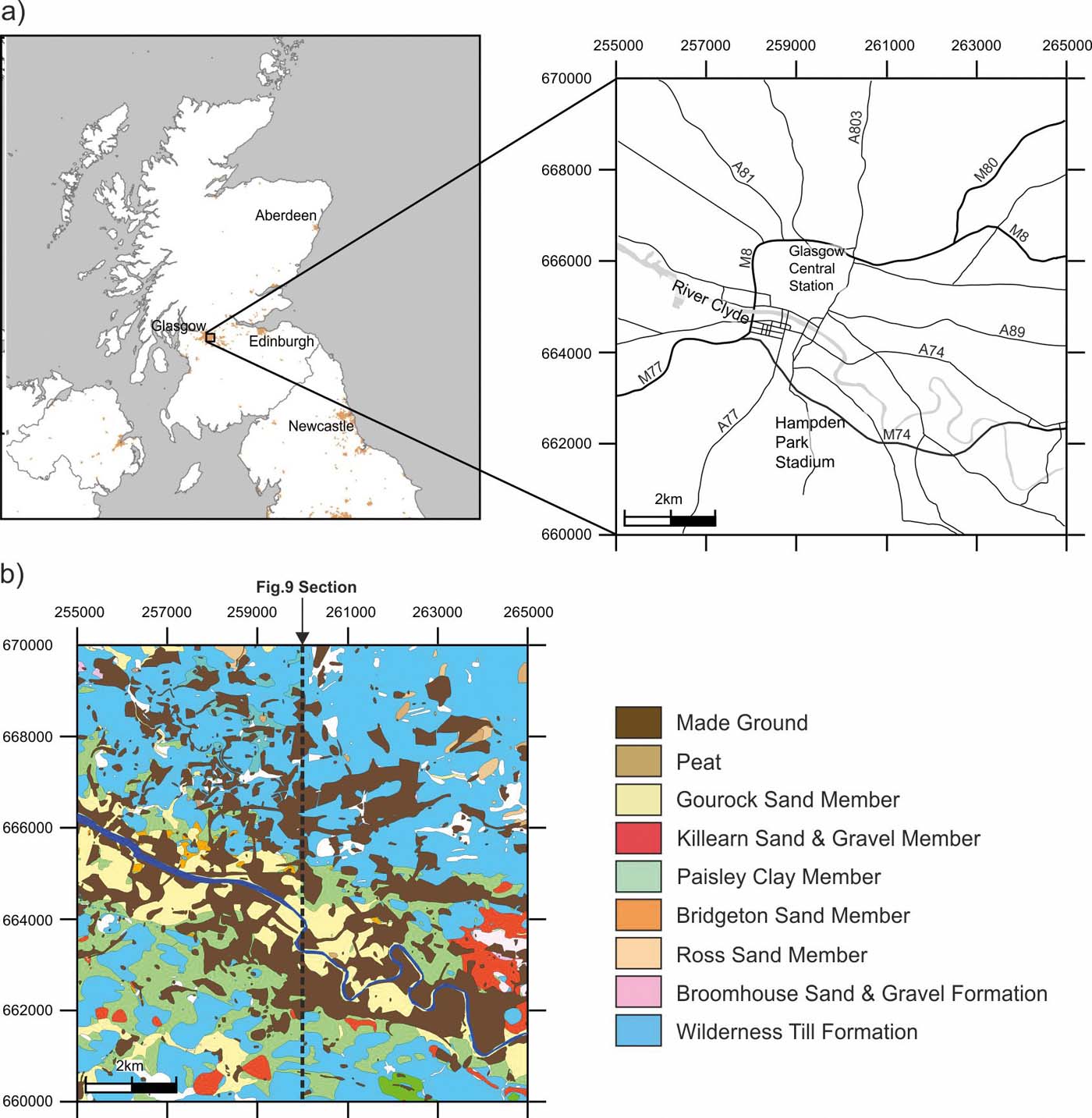
Figure 1 (a) Location of study area, showing River Clyde and major roadways. (b) Superficial geology map after Merritt et al. (Reference Merritt, Monaghan, Entwisle, Hughes, Campbell and Brown2007).
At least five glaciations are thought to have occurred in the Clyde Basin during the last 0.5Ma (Lee et al. Reference Lee, Busschers and Sejrup2012). Browne & McMillan (Reference Browne and McMillan1989), Finlayson et al. (Reference Finlayson, Merritt, Browne, Merritt, McMillan and Whitbread2010) and Finlayson (Reference Finlayson2012) provide a detailed account of the glacial cycles affecting the Clyde region and the associated lithostratigraphy, so only a brief description relevant to this study is outlined here. The superficial deposits of interest are the result of depositional processes during and following the last, Late Devensian, glacial maximum some 35,000 years BP (Brown et al. Reference Brown, Rose, Coope and Lowe2007; Jacobi et al. Reference Jacobi, Rose, MacLeod and Higham2009), which were deposited on a substrate of Carboniferous sedimentary and igneous rocks. The lithostratigraphic units are broadly divided into two sedimentological facies associations: glacial and post-glacial (Kearsey et al. Reference Kearsey, Williams, Finlayson, Williamson, Dobbs, Marchant, Kingdon and Campbell2015). The glacial facies includes the Wilderness Till Formation, the Cadder Sand and Gravel Formation, the Broomhill Clay Formation and the Baillieston Till, while the post-glacial facies consists of all remaining lithostratigraphic units overlying the Wilderness Till Formation (Kearsey et al. Reference Kearsey, Williams, Finlayson, Williamson, Dobbs, Marchant, Kingdon and Campbell2015). The Wilderness Till Formation, which comprises massive to locally stratified sandy silty clay diamicton, rests directly on bedrock in most of the study area, but in some areas rests on glaciofluvial sands and gravels, buried glaciolacustrine clays and/or the older Baillieston Till, where these are preserved within bedrock depressions. The post-glacial facies consists of subaqueous outwash-fan sand and gravel deposits, glaciomarine clays and fluvially influenced estuarine sands (Kearsey et al. Reference Kearsey, Williams, Finlayson, Williamson, Dobbs, Marchant, Kingdon and Campbell2015).
The lithostratigraphic units described above are highly heterolithic in nature, and it can be difficult to distinguish between them as there is often little or no visible lithological difference between units. Therefore, Kearsey et al. (Reference Kearsey, Williams, Finlayson, Williamson, Dobbs, Marchant, Kingdon and Campbell2015) utilised stochastic modelling techniques, more commonly employed by the oil and gas industry for reservoir modelling studies, to simulate the distribution of lithology within a cellular geological model (50×50×0.5m resolution) representing the superficial deposits in Glasgow. A key output of the Kearsey et al. (Reference Kearsey, Williams, Finlayson, Williamson, Dobbs, Marchant, Kingdon and Campbell2015) study was a suite of 500 different but equally probable simulations of the lithological variability across the model. These simulations are used here to condition stochastic simulations of the derived hydraulic conductivity within the model in order to eliminate some of the inherent lithological variability within the lithostratigraphic units. The model of Kearsey et al. (Reference Kearsey, Williams, Finlayson, Williamson, Dobbs, Marchant, Kingdon and Campbell2015) does not include the variable thickness of made ground, which cannot be accurately quantified in many parts of the city, and covers much of the superficial geology of the city. Therefore, this is not included in the model described here, though it is noted that made ground can exert an important control on shallow groundwater systems. Depending on local characteristics it can form either a barrier, or a preferential route for recharge and contamination, and/or it can be a contaminant source in itself (Fordyce et al. Reference Fordyce, Ó Dochartaigh, Bonsor, Ander, Graham, McCuaig and Lovatt2018; Ó Dochartaigh et al. Reference Ó Dochartaigh, Bonsor and Bricker2018). The component materials of made ground can either be waste such as masonry, derived locally from specific sites, or can be imported from further afield. Therefore, they are highly variable over short distances so their parameters are not geologically controlled. Separate analysis and modelling of the properties of made ground is recommended for future work.
2. Derivation of hydraulic conductivity
2.1. Methodology
Hydraulic conductivity has been derived from geotechnical data held by the British Geological Survey's National Geotechnical Properties Database (NGPD) (Self et al. Reference Self, Entwistle and Northmore2012), utilising the MacDonald formula (Eq. 1). The MacDonald formula uses d 10 and soil state description value (SSD) to derive hydraulic conductivity in units of mday–1.
The MacDonald equation (from MacDonald et al. Reference MacDonald, Maurice, Dobbs, Reeves and Auton2012) is:
 $$\log K = 0.79 \log d_{10} + (2.1 - 0.38 \rm SSD)$$
The d 10 is the maximum grain diameter (in millimetres) of the smallest 10 % by weight of particles obtained from a particle size distribution (PSD) test. The PSD test is a standardised geotechnical test (BS 1377-2:1990: British Standards Institution 1990) undertaken by passing a representative sample of material through a set of sieves ranging in aperture size from 75.00mm to 0.063mm.
Soil state directly describes relative density (for coarse soils) and consistency, which is indirectly related to density (for fine soils). SDD is routinely recorded when describing soils in accordance with British standards for site investigations (BS5930:1999: British Standards Institution 1999). The standard systematically describes the state of fine soils (silt and clay) from very soft through soft, firm and stiff to very stiff; and coarse soils (sand and gravel) from very loose through loose, medium dense, dense to very dense. For both coarse and fine soils, SSD is ranked from 1 for very loose and very soft soils through to 5 for very dense and very stiff soils (MacDonald et al. Reference MacDonald, Maurice, Dobbs, Reeves and Auton2012).
PSD data and SSD were extracted from the NGPD using an area search query, which returned all data within the confines of a square within British National Grid coordinates [255000,660000 265000,670000]. A total of 2,345 samples were found in the NGPD which contained XYZ coordinates, PSD and SSD data together with lithostratigraphic descriptions.
2.2. Alternative methods
In order to put the results of the MacDonald formula in context and verify whether it was the most appropriate method to use, comparison was made with derived values from six other formulae commonly used for predicting hydraulic conductivity from particle size data. Multiple formulae were evaluated.
The Hazen equation (after Vuković & Soro Reference Vuković and Soro1992) is:
 $$K = {\rm CH} d^2_{10} (0.7 + 0.03 \rm T)$$
where K is hydraulic conductivity in units of mday–1, CH is a coefficient after Hazen (Reference Hazen1892), assumed to be 1,000 and T is temperature in °C, assumed to be 10.
The Seelheim equation (after Vienken & Dietrich 2011) is:
 $$K = 0.00357 \times d^2_{50}$$
where K is hydraulic conductivity in units of ms–1 and d 50 is the diameter of the 50th percentile particle size (mm).
The United States Bureau of Reclamation (USBR) equation (after Vuković & Soro Reference Vuković and Soro1992) is:
 $$K = 0.36 d^{2.3}_{20}$$
where K is hydraulic conductivity in units of cms–1 and d 20 is the diameter of the 20th percentile particle size (mm).
The Beyer equation (after Vuković & Soro Reference Vuković and Soro1992) is:
 $$K = {\rm CB} d^{2}_{10}$$
where K is hydraulic conductivity in units of ms–1, d 10 is the diameter of the 10th percentile particle size (mm), CB is the Beyer coefficient (4.5×10⁻³ log(500/U)) and U is the coefficient of uniformity (d 60/d 10) where d 60 is the diameter of the 60th percentile particle size (mm).
The Kaubisch equation (after Vienken & Dietrich 2011) is:
 $$K = 10^{0.0005P2-0.12P-3.59}$$
where K is hydraulic conductivity in units of ms–1 and P is the percentage particle size<0.06mm.
The modified version of the Kozeny–Carman equation (after Odong Reference Odong2007; Barahona-Palomo et al. Reference Barahona-Palomo, Riva, Sanchez-Vila, Vasquez-Sune and Guadagnini2011; Bricker & Bloomfield Reference Bricker and Bloomfield2014):
 $$K_{\rm GSD} = 8.3 \times 10^{-3} (\rho_w g) / (\mu_w) (n^3 / (1 - n^2)) d^2_{10}$$
where ρ w is the density of water (at 10°C), g is the acceleration due to gravity, μ w is the dynamic viscosity of water (at 10°C), n is porosity, taken to be 0.255(1+0.83U) after Vuković & Soro (Reference Vuković and Soro1992), and U is the coefficient of uniformity (d 60/d 10).
All of the formulae have been developed for, or were derived from, material with a limited range of grain sizes. A summary of the application ranges and an assessment of these application ranges for the data extracted from the NGPD are presented in Table 1.
Table 1 Application ranges for different formulae used to derive hydraulic conductivity. The data within range (%) column shows the percentage of the available data from Glasgow that falls within the application ranges given.

Less than 11 % of the samples meet the application ranges for Hazen, USBR and Beyer, while less than 50 % meet the application range for Kaubisch and Kozeny–Carman. Neither the MacDonald nor the Seelheim equations have known restrictions on application; however, both were derived for lithologies with a range of grain size values – from clay to gravel in the case of MacDonald, and clay to sand in the case of Seelheim. For Seelheim, approximately 70 % of the samples do not contain significant amounts of gravel (here considered to be where >25 % of the sample is coarser than 2.00mm) and are therefore considered to be within the application range. For MacDonald, >82 % of the data from central Glasgow have a d 10 value within the range of d 10 values used to derive the formula, and are therefore considered to be within the application range.
Based solely on assessment of formula application range to the grain size of samples obtained from PSD data, the MacDonald formula is likely to be the most suitable for predicting the hydraulic conductivity of superficial deposits in central Glasgow. This is principally due to the wide range of grain sizes present, and in particular the high proportion of finer-grained material (silt and clay <0.06mm). The MacDonald formula is also considered particularly suitable for Glasgow because it uses a measure of relative density to account for changes in permeability associated with greater and lesser degrees of compaction. Therefore, it is likely to be more suitable for predicting hydraulic conductivity in environments where some superficial deposits have been subject to multiple glaciations, as is the case in Glasgow.
2.3. Analysis of derived hydraulic conductivity
Table 2 presents a summary of the hydraulic conductivity data derived using different formulae. Values calculated using the MacDonald formula have a near normal distribution and median values that fall in the centre of the population of medians derived from the other formulae, so are broadly representative of these. They also have the second smallest range, and better match the typical hydraulic conductivity values for common lithologies observed in Glasgow, as summarised in Lewis et al. (Reference Lewis, Cheney and Ó Dochartaigh2006). The majority of the outputs from other formulae have proven to be unsuited for samples with large ranges in grain sizes, as demonstrated by the improbable maximum values derived. For example, maximum hydraulic conductivity values calculated using the Hazen, Seelheim, USBR, Beyer and Kozeny–Carman formulae are far in excess of the typical values of 5–102 mday–1 for sand and gravel deposits given by Lewis et al. (Reference Lewis, Cheney and Ó Dochartaigh2006). Some formulae, in particular Beyer, are also ill-suited to very heterogeneous materials and even produce negative values where the uniformity coefficient is greater than 500. Therefore, the outputs from the MacDonald formula were used for the modelling process.
Table 2 Summary table showing derived hydraulic conductivity for the different formulae for all samples. Beyer produced negative values where d 60/d 10>500.

2.3.1. Comparison with in situ hydraulic conductivity
A limited number of in situ hydraulic conductivity data are also available, presented by lithostratigraphic unit (Bonsor et al. Reference Bonsor, Bricker, Ó Dochartaigh and Lawrie2010; Ó Dochartaigh et al. Reference Ó Dochartaigh, Bonsor and Bricker2018). The data comprise between 1 and 17 individual measurements for each of the five most widespread lithostratigraphic units: the Broomhouse Sand and Gravel Formation, Bridgeton Sand Member, Gourock Sand Member, Paisley Clay Member and the Wilderness Till Formation. These data were used to validate the derived hydraulic conductivity data with the proviso that lithostratigraphy does not necessarily provide a useful predictor of lithology, due to the heterolithic nature of the deposits in Glasgow (Kearsey et al. Reference Kearsey, Williams, Finlayson, Williamson, Dobbs, Marchant, Kingdon and Campbell2015). Hydraulic conductivity data derived using the MacDonald formula are summarised by lithostratigraphic unit in Table 3, and in box and whisker plots shown in Figure 2. The box plots (Fig. 2) demonstrate that the MacDonald formula produces hydraulic conductivity values with a much smaller distribution of values that are closer to the in situ hydraulic conductivity data than any of the other formulae for nearly every lithostratigraphic unit (including total range, interquartile ranges and median). This supports the findings of the application range analysis (Table 1) that the MacDonald formula is the most appropriate to use for the complex heterogeneous deposits underlying central Glasgow.

Figure 2 (a) Box and whisker plots for all data. (b–f) By lithostratigraphic formation. In situ hydraulic conductivity data (Bonsor et al. Reference Bonsor, Bricker, Ó Dochartaigh and Lawrie2010; Ó Dochartaigh et al. Reference Ó Dochartaigh, Bonsor and Bricker2018) are also shown for comparison within individual lithostratigraphic units.
Table 3 Summary table showing the hydraulic conductivity in units of mday–1 derived using the MacDonald formula, for the different lithostratigraphic formations. Abbreviations: BHSE = Broomhouse Sand and Gravel Formation; BRON = Bridgeton Sand Member; GUF = Gourock Sand Member; KARN = Killearn Sand and Gravel Member; LAW = Law Formation (now Clyde Valley Formation); MGR = Made Ground; PAIS = Paisley Clay Member; WITI = Wilderness Till Formation.

As only a limited number of in situ measured data are available, and those data that are available are not randomly distributed (potentially being biased towards sites with higher hydraulic conductivities), it is not possible to carry out a robust statistical validation of the derived hydraulic conductivity data. The highest number of in situ values were measured from the Gourock Sand Member (14) and the Paisley Clay Member (17), with only a single measurement from the Broomhouse Sand and Gravel Formation, six from the Bridgeton Sand Member and five from the predominantly fine-grained Wilderness Till Formation. A comparison of the available measured data against the derived data is shown in Figure 3, and generally shows a close comparison of the two distributions beneath the 70th percentile suggesting that the calculated values are representative of field observations. Above the 70th percentile, there are only a limited number of in situ measured data and they are biased to higher values, but are still within the range estimated from the derived data. This suggests that the calculated values are representative of all but highly permeable lithologies which have limited geographical extent (Kearsey et al. Reference Kearsey, Williams, Finlayson, Williamson, Dobbs, Marchant, Kingdon and Campbell2015).

Figure 3 (a) Cumulative frequency plots comparing derived and in situ measured hydraulic conductivity data, and histograms showing distribution of hydraulic conductivity data. (b) Derived using MacDonald formula. (c) Measured from in situ testing.
2.3.2. Comparison against lithological data
Kearsey et al. (Reference Kearsey, Williams, Finlayson, Williamson, Dobbs, Marchant, Kingdon and Campbell2015) developed a suite of stochastic models to investigate the distribution of lithology within the superficial deposits underlying Glasgow. Six lithological categories were used based on soil descriptions and PSD data: ‘Organic', ‘Soft Clay', ‘Stiff Clay Diamicton,' ‘Silt', ‘Sand' and ‘Sand and Gravel.' The lithology of the model domain is described by an array of discrete properties, attributing values to individual cells in the grid. The data and methodology used to generate the grid and its property attribution is described in detail by Kearsey et al. (Reference Kearsey, Williams, Finlayson, Williamson, Dobbs, Marchant, Kingdon and Campbell2015), and so is not repeated in detail here. Simulated properties include 500 unique, yet equally probable realisations of lithology. For the purposes of this study, they are each considered to be valid representations of the bulk lithology expected to occur within each discrete model cell. Furthermore, the use of multiple individual realisations rather than probability-based methods allows for the possibility that end-member lithologies could feasibly exist within any given cell in the absence of hard conditioning data, despite the low probability that such lithologies might occur at any given location.
In order to test whether these lithology simulations could be used to condition the hydraulic conductivity models, the corresponding lithology was recorded against each derived hydraulic conductivity measurement. A statistical summary of the derived hydraulic conductivity data for the different lithology classes is provided in Table 4.
Table 4 Summary statistics determined from raw hydraulic conductivity data (K), units are mday–1.

It can be seen from Table 4 that the mean values for the different lithology classes are consistent with expected hydraulic conductivity for different materials found in nature as given by Bear (Reference Bear1972) and Lewis et al. (Reference Lewis, Cheney and Ó Dochartaigh2006). The mean values for both the ‘Soft Clay' and ‘Stiff Clay Diamicton' classes are within the range given for unconsolidated layered clays, and the mean values for the ‘Silt', ‘Sand' and ‘Sand and Gravel' classes all fall within the range for well sorted sand or sand and gravels, although it is noted that due to the logarithmic nature of the classification given by Bear (Reference Bear1972) both ‘Silt' and ‘Sand' could justifiably also be described as falling within the upper range of the scale for very fine sand, silt, loess and loam. The mean values for the ‘Stiff Clay Diamicton' (Till), ‘Silt', ‘Sand' and ‘Sand and Gravel' all fall within the ranges given for common rock types by Lewis et al. (Reference Lewis, Cheney and Ó Dochartaigh2006). Together with the intuitive increase of the mean values with grain size, and the variation in material type and description (see Kearsey et al. Reference Kearsey, Williams, Finlayson, Williamson, Dobbs, Marchant, Kingdon and Campbell2015 for lithological descriptions), it is concluded that the distribution of hydraulic conductivity within the model domain can be based upon the previously simulated lithology properties.
3. Stochastic modelling
Grid-based conditional simulation was used to distribute the hydraulic conductivity data through a model domain, using the lithologically attributed grid described by Kearsey et al. (Reference Kearsey, Williams, Finlayson, Williamson, Dobbs, Marchant, Kingdon and Campbell2015). It would be equally possible to utilise unconstrained model volumes or lithostratigraphic models should lithological models be unavailable or deemed to be less appropriate for a given application. In this case, lithology was considered to be more suitable for constraining hydraulic conductivity distribution than lithostratigraphy, due to the intra-formational lithological variability inherent within the superficial deposits of Glasgow. Therefore, lithological descriptions better represent the grain size distribution, and subsequently the hydraulic conductivity in the subsurface, than lithostratigraphic determinations. In addition, as described by Kearsey et al. (Reference Kearsey, Williams, Finlayson, Williamson, Dobbs, Marchant, Kingdon and Campbell2015), the lithology models offer greater detail in terms of the geometry of individual litho-bodies and their geometrical relationships.
3.1. Input data and analysis
Derived hydraulic conductivity data were available from 603 boreholes within the model domain representing the superficial deposits, resulting in the data distribution shown in Figure 4. For many boreholes there were several measurements along their length. Data were provided in hydraulic conductivity (K) units of metres per day (mday–1), but have also been predicted by a transfer function to log10 conductivity, for which summary statistics for the different lithologies are shown in Table 5.
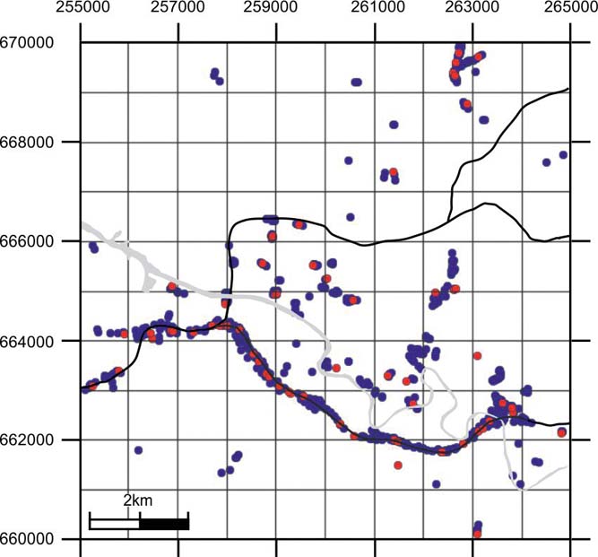
Figure 4 Distribution of boreholes for which hydraulic conductivity data are available. The red points are those boreholes where data has been excluded from the simulations to enable split-sample validation of the technique.
Table 5 Summary statistics determined from hydraulic conductivity data transposed to Log to base 10.

Residuals for the data were calculated by subtracting the measured values from the mean values shown in Tables 4 and 5, depending on the lithology class from which the measurements were derived, with residuals generated for both the original and for log conductivity. The distribution of residuals for the log conductivity data has a symmetrical, normal-looking distribution (Fig. 5), and on this basis is most suited to Gaussian simulation techniques. Therefore, the geostatistical analysis is based on log conductivity. The summary statistics for the log scale residuals (Table 6) do not suggest that there are any particular outliers in the data. The two skewness measures are in broad agreement, showing evidence of a mild positive skew, and the MAD (mean absolute deviation) scale statistic, which provides a robust measure of the standard deviation, is very close to the standard deviation.

Figure 5 Histogram showing the distribution of residual log hydraulic conductivity data.
Table 6 Summary statistics for the residual log hydraulic conductivity values in units of log10mday−1.

3.2. Spatial analysis
The program gamv3m from the GSLIB library (Deutsch & Journel Reference Deutsch and Journel1992) was used to obtain estimates of the empirical variogram from the data on conductivity. Estimates of the empirical variogram for four principal directions in the horizontal plane, with dip of zero and zero tolerance in Z (so that all comparisons are horizontal), were computed. Estimates were obtained with the conventional estimator of the variogram (Matheron Reference Matheron1962) and the GSLIB rodogram estimator. The latter was then rescaled to the Cressie–Hawkins (CH) robust estimator of the variogram (Cressie & Hawkins Reference Cressie and Hawkins1980). Exploratory variograms are shown in Figure 6. The CH variogram was included because it is more resistant to outlying observations than the conventional estimator. There is little evidence for anisotropy at shorter lags (up to about 2,000m), with the possible exception of direction 0, and there is also little difference between the two estimators. Therefore, isotropy (lack of dependence of the variogram on direction) is assumed in the horizontal plane.

Figure 6 Exploratory variogram estimates of the residual log hydraulic conductivity for four principal directions, 0 being N–S. Matheron estimates are solid symbols while Cressie–Hawkins are open.
In order to consider vertical variation, estimates of the variogram were then computed for a dip of 90°. The estimates showed mild spatial dependence down the borehole; therefore, models were considered with geometric anisotropy (isotropic in the horizontal plane, and an isotropy ratio, which is the ratio of the range of spatial dependence down the boreholes to the range in the horizontal plane). More information on the specification of directional dependence in variogram estimation is given by Deutsch & Journel (Reference Deutsch and Journel1992). Parameters for the variogram model were obtained by least squares fitting to the empirical variograms estimated with Matheron's estimator and the robust CH estimator. The fitted models are shown in Figure 7.

Figure 7 Fitted variogram models for (a) horizontal and (b) vertical directions. Matheron estimates are solid symbols while Cressie–Hawkins are open.
In order to obtain a final set of variogram parameters it was necessary to select between the model fitted to results from Matheron's estimator and the model fitted to results from the CH estimator. Cross-validation of the variograms was performed using GSLIB's xvkt3dm program. In cross-validation, each observation in turn is withheld from the data set and predicted by ordinary kriging. The predicted value of each observation and the ordinary kriging variance of the prediction are obtained. If the variogram model is sound, then the ordinary kriging variance is the expected mean squared error (MSE) of the kriging prediction (Lark Reference Lark2002). For each observation in the cross-validation we computed the standardised square kriging error (SSKE), which is the ratio of the squared error of the ordinary kriging predictor to the kriging variance. We then computed the mean and median of these values over all the data. Assuming normal kriging errors, the mean and median SSKE should be close to 1 and 0.455 respectively if the variogram gives a good description of the spatial dependence of the data and reliable kriging variances (Lark Reference Lark2002). The median is the more useful diagnostic, being less affected by outliers. In this case the mean and median SSKE for the Matheron estimator were 1.46 and 0.44 respectively. Those for the variogram obtained with the CH estimator were somewhat larger than expected (2.3 and 0.64 respectively), which may indicate a bias due to some non-normality of the underlying distribution. Therefore, on the criterion of selecting the model such that the median SSKE is closest to 0.455, we prefer the Matheron variogram, and use this in the simulation of the residual log hydraulic conductivity. The variogram parameters used are given in Table 7.
Table 7 Variogram parameters used in the simulation of the residual bulk density. The anisotropy ratio is 0.07324.

3.3. Stochastic simulation
The residual log hydraulic conductivity data were used to condition simulations of the property onto the grid using the ‘Reservoir Properties' workflow in GOCAD® 2009.4. Sequential Gaussian simulation, or SGS (Deutsch & Journel Reference Deutsch and Journel1992), was used to simulate 500 individual realisations of the property by variation of the random seed number, resulting in 500 unique realisations, one for each of the lithology simulations derived by sequential indicator simulation by Kearsey et al. (Reference Kearsey, Williams, Finlayson, Williamson, Dobbs, Marchant, Kingdon and Campbell2015). Data from 10 % of the boreholes were excluded from the simulations in order to provide a means of testing the workflow by comparison of the excluded data against the simulated values at those locations where validation data were present (Reference Bianchi, Kearsey and KingdonFig. 4). For each realisation of the hydraulic conductivity residual, we assigned a single realisation of lithology by adding the corresponding lithology class means (as given in Table 5) to the residual property. This provided 500 realisations of the hydraulic conductivity. Each individual realisation provides an equally probable representation of the spatial distribution of hydraulic conductivity through the model domain conditioned to the simulated lithology. Subsequently these were back-transformed to the original hydraulic conductivity units of mday–1.
The simulations all show a similar pattern of hydraulic conductivity distribution across the model area. Figures 8 and 9 show an example of one of the resulting simulations, alongside the corresponding simulation of lithology with which it is conditioned. It is clear that the highest hydraulic conductivities correspond to the River Clyde valley where the coarsest-grained lithologies predominate (Bianchi et al. Reference Bianchi, Kearsey and Kingdon2015; Kearsey et al. Reference Kearsey, Williams, Finlayson, Williamson, Dobbs, Marchant, Kingdon and Campbell2015). The slope areas, where glacial tills are most common, exhibit lower hydraulic conductivities, which is intuitive given the clay-rich nature of the stiff clay diamicton that constitutes the major component of the Wilderness Till Formation (Kearsey et al. Reference Kearsey, Williams, Finlayson, Williamson, Dobbs, Marchant, Kingdon and Campbell2015). More locally, the structure is dependent on the distribution of individual litho-bodies in the corresponding lithology simulations (Fig. 8).

Figure 8 (a) A single realisation of the distribution of hydraulic conductivity across the model domain. (b) The corresponding simulation of lithology. Note the distribution is dependent on both the gross distribution of lithofacies, while locally the structure is controlled by the distribution of simulated litho-bodies.

Figure 9 Cross-section showing distribution of (a) hydraulic conductivity from a single simulation and (b) the corresponding simulation of lithology. Location of section shown on Figure 1b. The black line represents the ground surface.
These individual simulations may be useful for specific purposes such as in the development of groundwater models. However, the particular value of the stochastic simulation approach is that multiple realisations may be interrogated in order to produce 3D probability distributions for identifying where the hydraulic conductivity values are likely to fall within, or to exceed given values. An example is shown in Figure 10 where the probability of values exceeding the 75th percentile of the simulated values (0.3mday–1) is shown. This value is within the range of division between poor and moderate productivity aquifers of ∼0.2–1mday–1 for Scottish aquifers of 10–50m thickness (Graham et al. Reference Graham, Ball, Ó Dochartaigh and MacDonald2009). The higher hydraulic conductivity values tend to be located along the present-day Clyde valley, although relatively higher probabilities of encountering moderately productive aquifers also exist in topographic depressions to the north and south of the study area. Some of these might be related to a late glacial marine flooding event and its subsequent retreat, where relative sea level rose to ∼40m above Ordnance Datum (Peacock Reference Peacock and Evans2003), leading to the deposition of coarse grained sediments in some topographic depressions at higher elevations.
A split-sample validation test was performed in order to assess the effectiveness of the stochastic modelling approach, with data from 10 % of the boreholes excluded from the simulations for use as validation points. For a non-spatial model where the hydraulic conductivity of the validation point locations is predicted as the mean log10 hydraulic conductivity of the dataset as a whole, the MSE between this estimate and the observed values is 1.36 (log10mday–1)2. If the mean log10 hydraulic conductivity is estimated based on the lithology of the validation points, the MSE is reduced by 60 %. Use of the spatial model presented here to estimate the hydraulic conductivity, reduces the remaining squared errors by a further 34 % at the validation point locations, suggesting that (1) lithology exerts an important control on the distribution of hydraulic conductivity in Glasgow, and (2) that the stochastic modelling technique presented here more accurately predicts the distribution of hydraulic conductivity than simple models based on bulk attribution of lithological models.

Figure 10 Probability of hydraulic conductivity exceeding 0.3mday–1, calculated from 500 individual simulations.
4. Discussions and conclusions
For the first time, an extensive hydraulic conductivity dataset for the superficial deposits across central Glasgow has been derived from geotechnical data acquired from site investigation boreholes. The method of MacDonald et al. (Reference MacDonald, Maurice, Dobbs, Reeves and Auton2012) has been used to generate the hydraulic conductivity data from PSD and SSD data. A range of alternative established formulae was also tested, but the data distribution of results from the MacDonald formula was found to match more closely the observed distribution of data from the limited number of in situ measurements, and was found to be the most appropriate to use in terms of the grain size application ranges of the different formulae. These data have been used to populate a 3D cellular model of the superficial deposits across central Glasgow with simulated hydraulic conductivity values. Five hundred unique realisations were produced, conditioned by previously simulated lithological distributions after Kearsey et al. (Reference Kearsey, Williams, Finlayson, Williamson, Dobbs, Marchant, Kingdon and Campbell2015).
The simulations indicate that the distribution of hydraulic conductivity values is strongly controlled by lithology, with higher values prevailing along the axis of the Clyde valley and within topographic lows where coarser grained deposits are more prevalent. The individual simulations are likely to prove difficult to implement explicitly within numerical groundwater models due to the large number of grid nodes and the requirement for upscaling (Nœtinger et al. Reference Nœtinger, Artus and Zargar2005). However, they are useful in obtaining a conceptual understanding of the distribution of flow properties across the region. Validation of the modelling technique was achieved by a split-sample validation test against a proportion of the hydraulic conductivity data excluded from the modelling workflow. This showed that as a predictive tool, the stochastic modelling results performed better by comparison with non-spatial models or models based-on bulk attribution.
This relationship between lithology and hydraulic conductivity is particularly important for understanding the variability of groundwater flow regimes in urban areas where the geology is largely hidden by development. Glasgow has a history of anthropogenic pollution and, in particular, buried wastes from historic heavy industry, and tracking such pollution is problematic. Improved understanding of the 3D geometry of potentially conductive aquifer units within the city will allow improved risk assessments for managing the legacy of pollutants. Previous conventional 2D geological modelling, or even more recent deterministic 3D modelling, does not provide sufficiently descriptive information to adequately discriminate the threats posed by the remobilisation of specific wastes. The techniques presented here provide a possible alternative, which may allow more locally focused models to be developed.
We demonstrate that geotechnical data can be used to produce a large and robust hydraulic conductivity dataset suitable for modelling and analysis of the distribution of hydraulic conductivity within the shallow subsurface across an area of 100km2 in central Glasgow [55.813°N–55.903°N; 4.157°W–4.319°W]. Stochastic attribution is achieved using a pre-existing voxellated (or geocellular) model representation of the superficial geology of Glasgow. Kearsey et al. (Reference Kearsey, Williams, Finlayson, Williamson, Dobbs, Marchant, Kingdon and Campbell2015) applied stochastic modelling techniques to generate models of the lithological variation within the superficial deposits in Glasgow, and those models form the foundation for this modelling study. The city of Glasgow is particularly suitable as a pilot study area to assess the suitability and robustness of the methodology as the underlying superficial deposits are highly complex and heterogeneous, and there are relatively few in situ hydraulic conductivity data available. Validation of the stochastic 3D modelling technique was achieved by withholding 10 % of the hydraulic conductivity data from the stochastic attribution so that it could later be compared to the modelled predictions. To the knowledge of the authors, this is the first account of a stochastic modelling approach aimed at studying the hydraulic conductivity of the shallow subsurface on a city-wide scale.
By developing a 3D model of the hydraulic conductivity of complex superficial deposits underlying a large city, we have shown that it is possible to understand the likely flow paths of groundwater in a complex sequence dominated by glacigenic, marine and estuarine deposits. This model will potentially facilitate an improved understanding of groundwater flow in 3D, reducing the spatial uncertainty of hydraulic parameters in groundwater process models.
The methodology applied here can be applied in any region where there is a good quantity and distribution of geotechnical data, which adequately characterises the variation of material properties, specifically particle size and relative density descriptions. While here it is applied to the central Glasgow area, it would also be of particular use in other urban areas in the UK and worldwide where superficial deposits are present and where the characterisation of controls on groundwater processes are important. A prerequisite is that detailed geological models are available to adequately describe the structure of the urban subsurface, providing a framework for property modelling.
5. Acknowledgements
Tim Kearsey and Ben Marchant are thanked for providing useful discussions on various aspects of this study. This paper was funded by NERC National Capability funding, and is published with the permission of the Executive Director, British Geological Survey (NERC). BGS/NERC reference: PRP17/052.


