


1. Introduction
Wake flows are not only of fundamental interest in scientific research but also of technical relevance since their fluid mechanical properties vastly influence aerodynamic properties of flight vehicles. Particularly at transonic to supersonic speed, base drag accounts for the major part of the total drag of an axisymmetric vehicle (Lamb & Oberkampf Reference Lamb and Oberkampf1995). Therefore, most previous work of primarily technical relevance has focused on strategies in order to increase supersonic base pressure, hence decreasing drag. This was almost exclusively realized by geometry modifications altering the wake flow structure, which is shown schematically in figure 1 for a wake flow separating from a circular cylinder aligned with the stream.

Figure 1. Schematic of the time-average supersonic wake flow behind an axisymmetric afterbody with truncated base.
As first described in detail by Chapman (Reference Chapman1950), the boundary layer separates at the corner, forming the free shear layer which undergoes an expansion and is also directed toward the symmetry axis. Approaching the central axis, the flow realigns with the free stream, resulting in the formation of a recompression shock in the outer wake. A part of the flow is not able to overcome the resulting adverse pressure gradient and is redirected toward the base, forming a recirculation region. The zero-axial-velocity line  $(U_x=0)$ which forms between the base and the rear stagnation point (RSP) separates the upstream-directed flow in the near wake from the far wake with its downstream-directed flow.
Extensive experimental studies on axisymmetric supersonic wakes at Mach 2.46 have been conducted by Herrin & Dutton (Reference Herrin and Dutton1994a), who measured radial base pressure distributions and mapped the flow field using laser Doppler velocimetry. Later, Kirchner et al. (Reference Kirchner, Favale, Elliot and Dutton2019) extended and refined the work by applying three-dimensional particle image velocimetry (PIV), allowing detailed statistics on turbulence and structural fluctuations. Although similar studies also demonstrating the effects of varying Mach and Reynolds numbers (Cope Reference Cope1953; Sieling & Page Reference Sieling and Page1970) can be found in the literature, the work of Herrin & Dutton (Reference Herrin and Dutton1994a) was most frequently used as a case for comparison against numerical simulations.
Early it was found that Reynolds-averaged Navier–Stokes (RANS) simulations are unable to predict the comparatively homogeneous radial base pressure distribution seen in the measurements (Dutton et al. Reference Dutton, Herrin, Molezzi, Mathur and Smith1995; Forsythe et al. Reference Forsythe, Hoffmann, Cummings and Squires2002). Numerous computational studies used the hybrid detached-eddy-simulation (DES) method, which models turbulence in the attached boundary layer while resolving large eddies far off walls temporally and spatially (Forsythe et al. Reference Forsythe, Hoffmann, Cummings and Squires2002; Kawai & Fujii Reference Kawai and Fujii2005; Barone & Roy Reference Barone and Roy2006). While this method led to vastly improved base pressure predictions, comparisons of the position of the RSP were generally in less agreement, with the trend of overly long recirculation regions observed in these simulations. The discrepancy can most likely be attributed to the non-physical transition of the turbulent boundary layer profile to a shear layer with physically resolved turbulence (Forsythe et al. Reference Forsythe, Hoffmann, Cummings and Squires2002; Simon et al. Reference Simon, Deck, Guillen and Sagaut2006, Reference Simon, Deck, Guillen, Sagaut and Merlen2007). Irrespective of numerical resolution, this non-physical transition can never be avoided using DES. Most recently, Sandberg (Reference Sandberg2012) approached the problem with a direct numerical simulation also resolving the turbulent structures in the attached boundary layer. Due to computational costs, however, the original Reynolds number of the flow analysed in the experiments of Herrin & Dutton (Reference Herrin and Dutton1994a) had to be reduced by a factor of 33. Despite the different flow condition, these computationally expensive simulations showed better agreement with the experiment, particularly with respect to the recirculation region length. As long as such simulations are not possible at matching flow conditions, high Reynolds number wake flow studies still warrant the need for experimental validation.
Thus, the most conclusive studies on wake flows resort to both numerical and experimental methods. As already mentioned, increasing the base pressure is of paramount technical interest. An effective and frequently implemented method therefore, boat-tailing the body divides the expansion into two parts (Sahu, Nietubicz & Steger Reference Sahu, Nietubicz and Steger1985; Herrin & Dutton Reference Herrin and Dutton1994b). Rough surfaces upstream of separation increase boundary layer momentum thickness, which in turn increases base pressure (Durgesh, Naughton & Whitmore Reference Durgesh, Naughton and Whitmore2013). While axisymmetric surface protrusions can have a similar effect (Bourdon & Dutton Reference Bourdon and Dutton2002), protrusions on distinct azimuthal positions alter the shear layer mixing properties, leading to lower base pressure (Bourdon & Dutton Reference Bourdon and Dutton2001; Janssen & Dutton Reference Janssen and Dutton2005). Another possibility to increase base pressure is based on adding base-mounted splitter plates protruding into the recirculation region (Reedy et al. Reference Reedy, Elliot, Dutton and Lee2012).
Weidner et al. (Reference Weidner, Hruschka and Albers2019a,Reference Weidner, Hruschka and Leopoldb) analysed the effect of axisymmetric swirl introduced by spinning vanes upstream of the separation of the boundary layer at the base corner, measuring decreased base pressure as a result of the rotation. This finding is of technical relevance, as many axisymmetric supersonic vehicles, such as projectiles, require axial spin for stabilization. The reason for the pressure changes observed still needs to be elucidated.
The current study extends the work of Weidner et al. (Reference Weidner, Hruschka and Leopold2019b) to higher spin rates, exploring the limits of the base pressure decrease. Also, as some previous numerical studies by Hruschka & Leopold (Reference Hruschka and Leopold2015) indicated spin-induced fundamental changes in the wake flow structure, the current work is aimed to corroborate and extend these results, with particular focus on fluid mechanical aspects. While the numerical DES simulations presented in this work provide a complete picture of the wake flow at different spin rates, their aforementioned shortcomings still warrant the need for additional measurements. Results from surface measurements such as pressure transducers, oil flow visualizations and pressure-sensitive paint (PSP) as well as planar PIV measurements for flow field analysis are presented to back up the simulations. The eventual aim is to provide convincing evidence for two fundamental changes of the wake flow structure occurring as a consequence of subsequently increasing axial spin rates.
2. Experimental set-up and methods
The experimental set-up of the present study, shown schematically in figure 2, is similar to the set-ups used in previous studies (Sieling & Page Reference Sieling and Page1970; Leopold Reference Leopold1993; Herrin & Dutton Reference Herrin and Dutton1994a; Augenstein et al. Reference Augenstein, Leopold, Christnacher and Bacher1999; Hruschka & Leopold Reference Hruschka and Leopold2015; Kirchner et al. Reference Kirchner, Favale, Elliot and Dutton2019; Weidner et al. Reference Weidner, Hruschka and Leopold2019b). The nozzle supply chamber is connected to a pressure reservoir supplying dry air at a stagnation pressure of  $4.8\times 10^5$ Pa and a stagnation temperature
  $T_0$ of 295 K. Upstream of the test section with a rectangular cross-section of
  $0.2 \textrm {m}\times 0.2 \textrm {m}$, shown in figure 3, the de Laval nozzle expanded the flow to an average free stream static pressure
  $p_\infty$ of
  $0.61\times 10^{5}$ Pa measured at the tunnel sidewall. The influence of the rectangular nozzle shape on the homogeneity of the central free stream flow was quantified by static pressure measurements 38.5 mm upstream of the base of a sting-mounted cylindrical reference geometry. The time-averaged static pressure at the four measured azimuthal positions – top, bottom, left and right – normalized by the total pressure in the nozzle supply chamber was measured to 0.1261, 0.1258, 0.1261 and 0.1264, respectively, with an uncertainty of
  $\pm$0.0025. In addition, the numerical simulations as described in § 4 show that the approach velocity 40 mm upstream of the base is uniform within 1 % in the free stream and within 5 % in the boundary layer. This indicates symmetric flow despite the axisymmetric model in the nozzle with rectangular cross-section. Still, some flow anisotropies within planes normal to the axis cannot be fully excluded. Based on the pressure ratios listed above, the free stream Mach number was calculated to be
  $2.01\pm 0.01$. This results in a Reynolds number
  $Re_{D}$ of
  $2.4\times 10^6$ based on the model diameter and the free stream conditions. The free stream turbulent intensity is estimated at less than 2 %, based on twice the standard deviation of the free stream velocities, obtained by the PIV method described in § 2.1.

Figure 2. Schematic of the afterbody model mounted in the nozzle supply chamber of the supersonic wind tunnel (Weidner et al. Reference Weidner, Hruschka, Rey, Leopold, Frohnapfel and Seiler2017).

Figure 3. Photography of the nozzle and the test section of the wind tunnel with the centred afterbody model and mounting sting.
The afterbodies were mounted on the axisymmetric sting centred in the wind tunnel. The sting and the nozzle geometry were designed using an axisymmetric and a two-dimensional method of characteristics, respectively. The solid body of the sting ideally replaces streamlines in the centre of the stingless nozzle, where the flow is nearly axisymmetric. In addition, the local boundary layer thickness, which was also calculated, was then deduced from the local sting radius and added to the local nozzle width, respectively. To reduce disturbances caused by the mounting structures, the sting was mounted in the nozzle supply chamber (Sieling & Page Reference Sieling and Page1970), as shown in figure 2.
The boundary layer thickness  $\delta$ resulting from the flow over the sting and the cylindrical model surface was measured 45.5 mm upstream of the base corner. A miniaturized Pitot probe was traversed through the boundary layer. Measurements between 1 and 11 mm surface distance clearly indicated a turbulent boundary layer with a thickness of 5 mm (Weidner et al. Reference Weidner, Hruschka and Leopold2019b; Weidner Reference Weidner2020), being in good agreement with values measured by Leopold (Reference Leopold1993) and Augenstein et al. (Reference Augenstein, Leopold, Christnacher and Bacher1999) for the same set-up.
Up to a length  $L_D$ of 135 mm upstream of the base corner, the diameter
  $D$ of the model was 40 mm. The Reynolds number
  $Re_L=\rho _\infty U_\infty L_\delta / \mu _\infty >8\times 10^6$ based on the streamwise dimension of the boundary layer
  $L_\delta >L_D$, the free stream velocity
  $U_\infty$ of 520 m s
 $^{-1}$, the free stream density
  $\rho _\infty =1.28~\textrm{kg m}^{-3}$ and the free stream dynamic viscosity
  $\mu _\infty =11.3\times 10^{-6}$ Pa s places the present wake flows in the turbulent regime (Chapman Reference Chapman1950; Kurzweg Reference Kurzweg1951).
The afterbody configurations of the present study, shown in figure 4, were equipped with 12 fins in order to obtain a relatively homogeneous flow without choking the flow between the fins. The 1 mm-thick fins extended from the base corner 20 mm upstream, having a height  $h_{f}$ of 12.5 mm extending through the boundary layer into the free stream. Table 1 lists the afterbody models of the present study with different fin-cant angles
  $\lambda$ as well as a cylindrical reference model without fins. Afterbodies having cant angles of 8
 $^\circ$ and 24
 $^\circ$ have been studied experimentally by Weidner (Reference Weidner2020).

Figure 4. Schematic of the used afterbody models having 12 canted fins (Weidner et al. Reference Weidner, Hruschka, Rey, Leopold, Frohnapfel and Seiler2017).
Table 1. Fin geometries of the afterbody configurations of the present study.

2.1. PIV
The axial and radial velocities in the vertical centreplane behind the afterbodies were measured with a two-dimensional, two component PIV method. Scarano & van Oudheusden (Reference Scarano and van Oudheusden2003) have shown that PIV methods – due to their nearly non-intrusive character (Tropea, Yarin & Foss Reference Tropea, Yarin and Foss2007) – are suitable for determining the velocities in a supersonic wake without significant alteration of the wake properties.
To seed the flow, a mixture of water and propylene glycol was evaporated and injected into the free stream upstream of the nozzle supply chamber. In order to increase the number of seeding particles in the flow region directly behind the afterbodies, additional seeding was needed. Therefore, a 2 mm-diameter central orifice in the model base was connected with a tube to the outside of the wind tunnel. The pressure difference between ambient conditions and the model base led to a mass flux into the recirculation region. This central mass flux was seeded with tobacco smoke primarily consisting of vaporized water, glycerol and glycol as well as solid particles (Rodgman & Perfetti Reference Rodgman and Perfetti2013). The effect of the seeding at the base centre on the measurement results is described in Appendix A.1.
The seeding particles in the flow were illuminated by a double-pulse frequency-doubled Nd:YAG laser system. The laser system was working with a repetition rate of 7 Hz and the time delay between the two successive pulses was 1  $\mathrm {\mu }$s. Each of the pulses had a duration of 10 ns, thus allowing the recording of instantaneous particle positions. The laser sheet in the vertical centreplane behind the afterbodies had an approximate thickness of 500
  $\mathrm {\mu }$m. The scattering of the light by the particles in the flow was recorded by a camera positioned perpendicular to the laser sheet, recording an individual image of
  $2048 \, \textrm {pixel}\times 2048 \, \textrm {pixel}$ resolution for each of the laser pulses.
During each wind-tunnel blow-down, 100 image pairs were recorded. The axial and radial velocities were calculated for each image pair with LaVision DaVis 10.1 (2020) using an equidistant evaluation grid with a node distance of 16 pixels and a spatial resolution of 38 evaluation nodes per base diameter  $D$. After two initial passes using correlation windows with an edge length of 48 pixels, four iterative passes using correlation windows with an edge length of 32 pixels and a Gaussian weighting function were performed.
Figure 5 shows the time-average axial and  $y$-Cartesian velocities,
  $\overline {U_x}$ and
  $\overline {U_y}$, normalized with the free stream velocity
  $U_\infty$ to
 \begin{equation} U_{x,PIV}^\star{=}\overline{U_x}/U_\infty\quad\text{and}\quad U_{y,PIV}^\star{=}\overline{U_y}/U_\infty \end{equation}
for the cylindrical afterbody without fins. The 95 % confidence uncertainty of the measured average flow velocities was calculated as described in Appendix A.1 to 1 % and 2 % of the free stream velocity in the outer and the inner wake, respectively.

Figure 5. Time-averaged relative velocities in the wake of the non-finned reference model resulting from PIV measurements – also plotted are the time-averaged streamlines, the expansion at the base corner (black dashed line), the recompression region (black dash–dotted line), the shock originating at the nozzle/test-section junction (black dotted line) and the zero-axial-velocity line  $\overline {U_x}=0$ (white solid line). (a) Axial velocities and (b)
  $y$-Cartesian velocities.
The PIV measurements for the non-finned cylinder are compared in table 2 with the experimental results of Leopold (Reference Leopold1993), Herrin & Dutton (Reference Herrin and Dutton1994a) and Kirchner et al. (Reference Kirchner, Favale, Elliot and Dutton2019). The axial position  $x_{RSP}$ of the RSP at
  $x/R\approx 2.86\pm 0.04$ was determined by the change of sign of the axial velocities along the central axis. The present experimental results for the normalized length of the recirculation region
  $x_{RSP}/R$, defined by the position of the RSP and the base radius
  $R$, agree with the results of Leopold (Reference Leopold1993) within their uncertainties. In contrast to that, the results of Herrin & Dutton (Reference Herrin and Dutton1994a) and Kirchner et al. (Reference Kirchner, Favale, Elliot and Dutton2019) show a shorter length of the recirculation region since they had been carried out at a higher free stream Mach number of 2.46 and 2.49, respectively (Murthy & Osborn Reference Murthy and Osborn1976). The normalized positions of the maximum upstream velocity,
  $x|_{\min{U_x^\star}}/x_{RSP}$, however, are in good agreement with the PIV measurements of the present study. Additionally, the maximum reverse flow velocity,
  $\min {U_x^\star }$, of
  $-0.257\pm 0.007$ measured for the non-finned afterbody agrees well with the experimental data of Leopold (Reference Leopold1993), Herrin & Dutton (Reference Herrin and Dutton1994a) and Kirchner et al. (Reference Kirchner, Favale, Elliot and Dutton2019).
Table 2. Comparison of the RSP position, the maximum, relative upstream velocity and its relative position determined by experimental means in axisymmetric wake flows at free stream Mach numbers of 2.0 and 2.5.

The wake pattern in figure 5 is of comparable symmetry as the results of Kirchner et al. (Reference Kirchner, Favale, Elliot and Dutton2019). This was achieved by a careful alignment of the model with the free stream using surface oil flow visualizations. For the finned models, the symmetry of the flow was of similar quality. Therefore, the resulting velocities for each image pair of the finned models were transformed from Cartesian coordinates  $(x,y)$ to cylindrical coordinates
  $(x,r=|y|)$. Thus, an average of up to 800 instantaneous measurements was calculated from 400 image pairs recorded during four blow-downs for each of the finned models. For these finned models, the uncertainties of the average velocities – also based on a confidence level of 95 % – were determined according to Appendix A.1 to typically less than 1 % and 4 % of the free stream velocity in the outer and the inner wake, respectively.
2.2. Pressure measurements
2.2.1. PSP
The static pressure at the model surface was measured by applying PSP. This method is capable of determining the pressure distribution with a high spatial resolution, thus rendering it suitable to visualize the shock footprints caused by the fins.
For the present PSP measurements, platinum porphyrin molecules (PtTFPP) within an oxygen-permeable matrix were applied to the model surface. The electrons of the porphyrin complexes were excited to a higher energy level by a continuous light source of  $(400\pm 15)$ nm wavelength. After the excitation, the electrons returned to their original energy level by either emitting a photon of a wavelength between 620 and 750 nm, or by transferring the excess energy to an oxygen molecule of the surrounding air flow. Hence, the intensity of the emitted light is dependent on the local oxygen concentration, which itself is proportional to the local pressure. Higher pressures result in a higher oxygen concentration, thus leading to a lower intensity of the emitted fluorescence. Therefore, the emitted light was imaged with a camera using a bandpass filter of
  $(650\pm 10)$ nm blocking the scattered light resulting from the excitation of the porphyrin molecules. The local pressure on the model surface was then evaluated using the Stern–Volmer relation
 \begin{equation} \frac{I_{ref}}{I}=A+B\frac{p}{p_{ref}}, \end{equation}
with the coefficients  $A$ and
  $B$ being dependent on the present temperature and the used PtTFPP molecules (Stern & Volmer Reference Stern and Volmer1919). As a reference, the intensity
  $I_{ref}$ of the emitted light was recorded directly after each blow-down since the model temperature was then similar to the conditions during the blow-down. The reference pressure
  $p_{ref}$ at the model surface was then equal to the ambient pressure. The pressures
  $p$ during each wind-tunnel blow-down were evaluated from the measured fluorescence intensities
  $I$ during the individual wind-tunnel runs and the corresponding reference measurements (Martinez Reference Martinez2007). The temperature gradients due to the shock waves caused by the fins, and the changing excitability of the molecules caused by the ambient-air humidity (Tropea et al. Reference Tropea, Yarin and Foss2007) to which the PtTFPP molecules were exposed between the individual blow-downs, however, limited the usage of the obtained results to qualitative comparisons.
Figure 6 shows the time-average pressure distribution at the surface of the non-finned afterbody with a mean value of  $0.66\times 10^5$ Pa. This value is 8 % higher compared with the previously mentioned static pressure measurements using pressure transducers at
  $x/R=-1.925$ and different azimuthal positions (Weidner et al. Reference Weidner, Hruschka and Leopold2019b) which are in good agreement with the expected pressures resulting from isentropic flow theory.

Figure 6. Pressure-sensitive paint measurement at the model surface upstream of the base corner of the non-finned reference model.
2.2.2. Base pressure
The pressure on the model base was measured with miniature pressure transducers (Kulite 2014) integrated in the model base. The transducers were mounted at different radial positions behind 3 mm-deep orifices having a diameter of 1 mm. The orifices were distributed on the base as indicated in figure 7. One transducer was mounted on the central orifice with a larger diameter of 2 mm, also used for the particle seeding during the PIV measurements.

Figure 7. Positions of the pressure measurement orifices at the model base (dimensions given in mm).
The pressure at the base  $p_{b}$ was normalized with the free stream static pressure
  $p_\infty$, resulting in the relative base pressure
  $p_{b}^\star$. This way, the effect on the base pressure caused by the increase of the free stream pressure of up to 2 % during the typical blow-down duration of 40 s was corrected for.
Figure 8 shows the average of the measured normalized base pressures at various radial positions for the non-finned afterbody. The error bars indicate the uncertainty interval with a confidence level of 95 % as calculated in Appendix A.2. The measurement results show an average deviation of 3.5 % from the measurements of Leopold (Reference Leopold1993) using the same wind-tunnel set-up and a similar afterbody with a smaller diameter of 38.66 mm. The deviations between the present measurements and the results of Leopold (Reference Leopold1993), however, are of the order of magnitude of the average experimental uncertainty of 3.4 %. Since the deviations primarily originate from the temperature dependency of the transducers mounted in the model, the central base pressure was additionally measured with a transducer (GE Sensing 2007) mounted outside of the wind tunnel and connected to the orifice at the base centre using the tubing of the PIV seeding. The measurements of the external transducer and the model-integrated central transducer deviated by 1.6 %, thus corroborating the estimated error margin for the results obtained with the built-in transducers.

Figure 8. Measured, time-averaged, radial base pressure profile of the non-finned reference model in comparison with the experimental results of Leopold (Reference Leopold1993).
3. Experimental results
3.1. Wall-shear stress visualizations
Figure 9 shows the wall-shear stress visualizations (Maltby Reference Maltby1962) of the finned afterbodies also used for the alignment of the models with the free stream flow. The flow pattern at the base of the afterbody with a fin-cant angle  $\lambda$ of 0
 $^\circ$, shown in figure 9(a) and shown in the supplementary movie 1 available at https://doi.org/10.1017/jfm.2021.465, is nearly axisymmetric, thus showing that the asymmetries in the free stream due to the rectangular nozzle shape had no relevance for the present study. The radial flow direction from the base centre to the base corner is typical for the classical supersonic turbulent wake flow (Herrin & Dutton Reference Herrin and Dutton1994a).

Figure 9. Oil flow visualizations of the velocity field in the vicinity of the surface of afterbody models with different fin-cant angles  $\lambda$ (Weidner et al. Reference Weidner, Hruschka, Rey, Leopold, Frohnapfel and Seiler2017): (a)
  $\lambda =0^\circ$; (b)
  $\lambda =16^\circ$; (c)
  $\lambda =32^\circ$.
The zones around the fins into which the oil could not intrude coincide with the footprints of the horseshoe vortices (Dolling & Bogdonoff Reference Dolling and Bogdonoff1980) illustrated in figure 10. Moreover, it is shown in figure 10 how the shock waves caused by neighbouring fin leading edges intersect between the fins. Afterward, the shock waves are interacting with the boundary layer at the fin surface, resulting in a local separation of the flow visible in figure 9(a) and movie 1.

Figure 10. Illustration of the horseshoe vortices generated at the fin leading edges.
Figure 9(b) and movie 2 show a helical pattern on the base of the afterbody having fins with a cant angle,  $\lambda$, of 16
 $^\circ$. The azimuthal deflection of the oil toward the axis is a result of the swirling flow motion introduced by the canted fins and transported into the flow region directly downstream of the afterbody. In addition to the azimuthal deflection, the radial direction of the flow adjacent to the base has changed as it is indicated by the oil accumulation at the base centre. Hence, figure 9(b) and movie 2 show a first experimental evidence of the changed wake flow structure due to swirl as it has been predicted by the numerical simulations of Hruschka & Leopold (Reference Hruschka and Leopold2015).
For the afterbody having a fin-cant angle,  $\lambda$, of 32
 $^\circ$, the wall-shear stress visualization in figure 9(c) and movie 3 show an annular oil accumulation with
  $r/R\approx 0.8$ at the base. At the position of the oil accumulation, the flow adjacent to the model base separates from the base, resulting in a wake flow structure not yet described in the literature. Despite the fin-cant angle of 32
 $^\circ$, the oil pattern at the base does not show any circumferential deflection of the oil flow, thus suggesting low circumferential flow velocities in the wake compared with the afterbody with
  $\lambda =16^\circ$. This becomes even more evident when observing the displacement of the oil over time in the video recordings in movies 2 and 3.
3.2. Axial and radial flow velocities in the wake
Figures 11 and 12 show the measured time-average axial and radial flow velocities normalized by the free stream velocity in the wake of the finned afterbodies. The axial velocity downstream of the fins is of the order of magnitude of the free stream velocity, thus indicating that the fins do not choke the flow. The axial velocity downstream of the fins of the afterbody with  $\lambda =32^\circ$ shown in figure 11(c), however, is decreased by approximately 10 % compared with the afterbody with non-canted fins.

Figure 11. Time-averaged, relative, axial velocities in the wake of the finned afterbody models resulting from PIV measurements – also plotted are the time-averaged streamlines, the fin leading-edge shocks (black solid line), the expansion at the base corner (black dashed line), the recompression region (black dash–dotted line), the shock originating at the nozzle/test-section junction (black dotted line), the zero-axial-velocity line  $\overline {U_x}=0$ (white solid line), the counter-rotating vortices ((1), (2)) and the downstream-directed vortex tube (3) (Weidner et al. Reference Weidner, Hruschka, Rey, Leopold, Frohnapfel and Seiler2017). Here (a)
  $\lambda =0^\circ$; (b)
  $\lambda =16^\circ$; (c)
  $\lambda =32^\circ$.

Figure 12. Time-averaged, relative, radial velocities in the wake of the finned afterbody models resulting from PIV measurements – also plotted are the time-averaged streamlines, the fin leading-edge shocks (black solid line), the expansion at the base corner (black dashed line), the recompression region (black dash–dotted line), the shock originating at the nozzle/test-section junction (black dotted line), the zero-axial-velocity line  $\overline {U_x}=0$ (white solid line), the counter-rotating vortices ((1), (2)) and the downstream-directed vortex tube (3) (Weidner et al. Reference Weidner, Hruschka, Rey, Leopold, Frohnapfel and Seiler2017). Here (a)
  $\lambda =0^\circ$; (b)
  $\lambda =16^\circ$; (c)
  $\lambda =32^\circ$.
The velocity fields of figures 11(a) and 12(a) downstream of the afterbody with non-canted fins show a recirculation region that is typical for turbulent supersonic wakes. In comparison with the non-finned afterbody, oblique shock waves are present in the outer wake, resulting from the shock waves caused by the fin leading edges. The RSP for the afterbody with non-canted fins is located at  $x/R=2.88\pm 0.02$. Hence, the non-canted fins result in a slightly larger recirculation region compared with the non-finned cylinder. This is due to the reduced Mach number at the base shoulder caused by the compression of the flow due to the presence of the fins, thus resulting in a higher relative base pressure (Lamb & Oberkampf Reference Lamb and Oberkampf1995). Hence, the expansion at the base corner is weaker and the deflection of the flow toward the central axis is less pronounced.
The maximum upstream velocity for the afterbody with non-canted fins is located on the central axis at  $x/R=1.46\pm 0.05$, and thus 13 % closer to the base than for the non-finned afterbody. In addition, the magnitude of the normalized maximum upstream velocity of
  $0.262\pm 0.007$ measured for the afterbody with non-canted fins is 2 % higher than for the non-finned afterbody. The resulting increase of the upstream mass flux is due to the horseshoe vortices enhancing the entrainment of the fluid in the recirculation region by the shear layer (Bourdon & Dutton Reference Bourdon and Dutton2001; Janssen & Dutton Reference Janssen and Dutton2005).
Despite the change of up to 13 % in the position of the maximum upstream velocity, the flow fields of the non-finned afterbody and the afterbody with the non-canted fins are generally similar. Hence, the presence of the non-canted fins does not result in a substantial change of the wake structure.
For the afterbody with 16 $^\circ$-canted fins, figure 11(b) shows that the flow detaching from the base corner does not reach the central axis. The outer flow becomes realigned with the axis of the flow field at
  $x/R\approx 1.5$ and
  $r/R\approx 0.6$. Downstream of the recompression the shear layer is, however, closer to the central axis than it has been when separating at the base corner. Hence, the conservation of angular momentum results in high azimuthal velocities of the fluid, decreasing the number of seeding particles close to the axis. Thus, it has not been possible to obtain reliable PIV results close to the axis for
  $x/R>3$, as is shown by the regions without measurement data in figures 11(b) and 12(b).
The adverse pressure gradient caused by the recompression shock redirects parts of the shear layer toward the base of the afterbody, as shown in figure 11(b). Thus, an upstream flow establishes in the wake of the afterbody with  $16^\circ$-canted fins having a maximum normalized velocity of
  $-0.157\pm 0.007$ at
  $x/R=0.34\pm 0.05$. In contrast to the non-finned afterbody and the afterbody with non-canted fins, the maximum upstream velocity is not located at the axis but at a radial position of
  $r/R=0.66\pm 0.05$. Neglecting the azimuthal velocity component that could not be measured with the used PIV method, the upstream flow together with the downstream directed shear layer forms an outer toric vortex
  surrounding a counter-rotating inner toric vortex
  shown in the time-averaged flow fields of the figures 11(b) and 12(b). As it has also been shown in figure 9(b), the inner toric vortex
 ![]() results in a reversal of the radial flow direction at the base compared with the classical wake flow. As a result, the flow separates at the base centre leading to a central downstream-directed flow
results in a reversal of the radial flow direction at the base compared with the classical wake flow. As a result, the flow separates at the base centre leading to a central downstream-directed flow  . The downstream-directed flow at the axis thus forms the vortex tube simulated by Hruschka & Leopold (Reference Hruschka and Leopold2015) and in § 5 of the present paper.
In contrast to the afterbody with  $16^\circ$-canted fins, a fin-cant angle of
  $32^\circ$ as shown in figure 11(c) results in an upstream directed flow at the central axis. The normalized maximum upstream velocity of
  $-0.32\pm 0.01$ at
  $x/R=1.25\pm 0.10$ is again located on the axis. As shown later, this flow is at low density, thus limiting its importance. Only in the vicinity of the base a local region with a downstream-directed flow is present close to the axis caused by the local effects of the PIV seeding at the base centre. The shear layer downstream of the afterbody with
  $32^\circ$-canted fins is only weakly deflected toward the central axis and the recompression realigns the flow to the axis already at
  $x/R\approx 1$ and
  $r/R\approx 0.8$. Due to the small deflection angle toward the axis, the Mach number perpendicular to the recompression shock is lower than for the afterbody with
  $16^\circ$-canted fins, resulting in a lower adverse pressure gradient in the shear layer. Hence, most of the fluid in the shear layer is capable of overcoming the pressure gradient and hardly any fluid is directed back to the base. Thus, the shear layer convects downstream forming a vortex tube enclosing a low-momentum inner flow region. Similar to the classical wake, the upstream flow at the central axis is a result of the mass entrainment by the shear layer and the conservation of the mass in the inner-wake region. The highly swirling outer flow in conjunction with the low-momentum inner-wake region having a near-zero azimuthal velocity component bears similarity to the interaction of vortex tubes with shock waves in supersonic flow fields (Délery et al. Reference Délery, Horowitz, Leuchter and Solignac1984; Settles & Cattafesta Reference Settles and Cattafesta1993), as is further discussed in Appendix B.
In addition, figure 12 shows that the compression shocks caused by the flow deflection at the fins result in a stronger radial deflection of the outer flow with increasing fin-cant angle. For a fin-cant angle of  $32^\circ$, the compression shocks themselves are not visible in figures 11(c) and 12(c) since the location of the detached shock is farther upstream for higher cant angles, as has been shown in figure 9.
3.3. Pressure measurements
3.3.1. Static pressure at the model surface
Figure 13(a–c) show the static pressure  $p$ on the model surface normalized with the free stream pressure
  $p_\infty$ for the different fin-cant angles
  $\lambda$ measured with the PSP technique. With increasing fin-cant angle
  $\lambda$, the detached shocks upstream of the fin leading edges result in a higher pressure on the model surface and an upstream shift of the shock position, which is also visible in figures 9 and 12.

Figure 13. Time-averaged pressure distribution, normalized with the free stream pressure  $p_\infty$, at the cylindrical model surface and the fin surfaces of the afterbody models with different fin-cant angles obtained with the PSP method –
  $\unicode{x24B6}$ interaction of the fin leading-edge shock with the fin boundary layer,
  $\unicode{x24B7}$ detachment shock,
  $\unicode{x24B8}$ right-leg shock of the shock wave–boundary layer interaction caused by the fin leading-edge shock,
  $\unicode{x24B9}$ expansion due to the fin wake,
  $\unicode{x24BA}$ recompression due to the fin wake,
  $\unicode{x24BB}$ compression due to the fin leading edge,
  $\unicode{x24BC}$ expansion due to the fin leading edge. Here (a)
  $\lambda =0^\circ$; (b)
  $\lambda =16^\circ$; (c)
  $\lambda =32^\circ$; (d)
  $\lambda =0^\circ$ with cylindrical model extension; (e)
  $\lambda =16^\circ$ with cylindrical model extension; (f)
  $\lambda =32^\circ$ with cylindrical model extension.
The high pressure immediately upstream of the fin leading edge in figure 13(a) is due to the right-leg shock of the shock wave–boundary layer interaction (Dolling & Bogdonoff Reference Dolling and Bogdonoff1980). On the fin surface, the footprint of another shock wave–boundary layer interaction is visible resulting from the interaction of the fin leading-edge shock with the fin boundary layer. Downstream of this interaction, the boundary layer re-establishes, thus matching the pressure directly upstream of the base corner to the free stream pressure level.
In contrast to the model with  $\lambda =0^\circ$ with its symmetrical flow around the fins, the cant angle of the fins results in an increased pressure on the windward side and a decreased pressure on the leeward side of the fins as shown in figure 13(b,c).
For the model with  $\lambda =16^\circ$, the expansion and compression forming at the leading edge of two neighbouring fins interact with each other upstream of the fin trailing edges. Hence, the flow on the suction side of the fins is compressed and the flow on the pressure side is expanded. Thus, the pressure differences level off upstream of the base corner.
Since the fin-cant angle  $\lambda =32^\circ$ is larger than the Prandtl–Meyer angle of
  $26^\circ$ for a flow Mach number of
  $2$, the flow separates on the suction side of the fins directly at the leading edge. Hence, the flow cross-section between the fins is reduced compared with the model with
  $\lambda =16^\circ$ and the detached shocks upstream of the fin leading edges increase in strength. This, in turn, results in the upstream shift of the separation shock footprint on the model surface shown in figure 13(c).
To investigate the effect of the flow between the fins on the pressure immediately upstream of the flow separation at the base corner, a 30 mm long cylindrical extension was attached to the different models. The extension had the same diameter as the models. As it is shown in figure 13(d–f), the model extension does not alter the flow between the fins.
In figure 13(d), the measured surface pressure distribution for the model with  $\lambda =0^\circ$ with extension is shown. The local expansion downstream of the fin trailing edges is caused by the finite thickness of the fins. The average pressure downstream of the fin trailing edges (
 $0< x/R<0.5$) is 10 % lower than upstream of the fins.
For a fin-cant angle of  $16^\circ$, the average pressure downstream of the fin trailing edges is 30 % lower than upstream of the fins, as shown in figure 13(e). This is due to the stronger detached shock upstream of the fins as well as due to azimuthal flow velocities resulting in a radial flow deflection, hence reducing the surface pressure. The shocks and expansions originating from the fin leading edges, which are reflected from the fins, result in the characteristic pressure pattern on the cylindrical model extension.
For the model with  $\lambda =32^\circ$, figure 13(f) shows a decrease of the average pressure downstream of the fins of 50 % compared with the free stream pressure. The larger pressure decrease compared with the model with
  $\lambda =16^\circ$ results from the flow separation at the fin leading edges amplifying the detached shock upstream of the fins. In addition, the increase of the azimuthal velocities results in an enhanced radial flow deflection compared with the model with
  $\lambda =16^\circ$ which further decreases the pressure downstream of the fins.
Overall, the surface pressure measurements show that the canted fins decrease the static pressure in the plane of the fin trailing edges.
3.3.2. Base pressure
In figure 14, the measured radial base pressure profiles for the finned models are shown and compared with the non-finned model. The absolute measurement uncertainties – calculated as described in Appendix A.2 – have the same order of magnitude as for the non-finned model.

Figure 14. Measured, time-averaged, radial base pressure profile of the finned afterbody models in comparison with the non-finned reference model (Weidner et al. Reference Weidner, Hruschka, Rey, Leopold, Frohnapfel and Seiler2017).
For the model with non-canted fins, the pressure decrease of 10 % in the fin trailing edge plane, shown in figure 13(d), is counteracted by the reduced Mach number at the base corner due to the presence of the fins. The lower Mach number at the base corner results in a higher base pressure compared with the pressure at the base corner (Lamb & Oberkampf Reference Lamb and Oberkampf1995). The effects of the decreased pressure at the base corner and the horseshoe vortices (Bourdon & Dutton Reference Bourdon and Dutton2001) are, however, larger, thus resulting in an overall base pressure decrease of 6 % compared with the non-finned model. Hence, the alteration of the base pressure is within the range of 5 % to 10 % given by Moore, Hymer & Wilcox (Reference Moore, Hymer and Wilcox1992) for the fins of the present study with a length-to-thickness ratio of 20 and the present free stream Mach number of 2.
The radial pressure profile of the model with  $\lambda =16^\circ$ shows for
  $r/R>0.5$ a pressure decrease of 50 % compared with the model with non-canted fins, resulting from the decreased pressure upstream of the base corner. In addition, the base pressure profile for the model with
  $\lambda =16^\circ$ shows a radial pressure gradient at
  $r/R<0.5$ caused by the azimuthal velocities
  $U_\varphi$ in the wake, visualized in figure 9(b), and hence resulting in a pressure minimum at the base centre. This pressure distribution is similar to those found in gas centrifuges (Kemp Reference Kemp2009), which can be described by
 \begin{equation} \frac{\partial p}{\partial r}=\rho \frac{U_\varphi^2}{r}. \end{equation}
 Compared with the model with  $\lambda =16^\circ$, the average base pressure for the model with a fin-cant angle of 32
 $^\circ$ has the same order of magnitude. The base pressure is decreased by 50 % compared with the model with non-canted fins – in comparison with the model with
  $\lambda =16^\circ$, however, there is no distinct radial pressure gradient. This is in agreement with the observations in figure 9(c) indicating low azimuthal velocities in the wake compared with the pronounced helical pattern for the model with
  $\lambda =16^\circ$.
3.4. Summary of experimental results
In the present experiments, the three distinctively different wake flow structures, as sketched in figure 15, were observed. The schematics are constructed by a synthesis of the individual experimental results and will be backed up by the results of the numerical simulations in §§ 5 and 6. The movies 4 to 6 show animations of the simulated, time-averaged flow fields for the different model configurations.

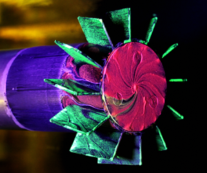
Figure 15. Illustrations of the time-averaged wake structures for the different fin cant angles  $\lambda$, as observed in the experiments and backed up by the time-averaged results of the numerical simulations shown in § 4 and animated in the movies 4 to 6; the colour of the ribbons indicates the flow velocity. Here (a)
  $\lambda =0^\circ$; (b)
  $\lambda =16^\circ$; (c)
  $\lambda =32^\circ$.
For a fin-cant angle  $\lambda$ of
  $0^\circ$, the time-average flow field illustrated in figure 15(a) corresponds to the classical supersonic wake flow of a non-finned axisymmetric afterbody. In comparison with the experimental data for the non-finned afterbody, the base pressure is decreased by 6 % due to the presence of the fins.
Figure 15(b) shows a sketch of the wake structure observed for the model with  $\lambda =16^\circ$. The swirling flow detaches at the base corner and is deflected toward the central axis due to the lower pressure at the base compared with the free stream. The centrifugal forces, present in a non-inertial reference frame rotating with the fluid around the central axis, increase when the flow approaches the central axis. Thus, the streamwise pressure gradient resulting from the radially converging flow also increases due to the centrifugal forces. As a result of this streamwise pressure gradient, a part of the shear layer is redirected toward the base before reaching the central axis. This, in turn, results in the outer toric vortex shown in figure 11(b). The counter-rotating, inner toric vortex results in the observed change of the radial flow direction at the base compared with the classical wake flow due to the vanishing centrifugal forces in the vicinity of the base surface. The additional circumferential flow velocity leads to the helical pattern on the base visualized in figure 9(b) and illustrated in figure 15(b). The flow detaches at the base centre, thus resulting in a downstream-directed central vortex tube with low axial momentum.
The sketched flow field for  $\lambda =32^\circ$ in figure 15(c) shows a flow detaching at the base corner which is only marginally deflected toward the central axis as observed in the PIV measurements. In contrast to lower fin-cant angles, the streamwise pressure gradients are hence negligible and most of the fluid is capable of flowing downstream without redirection to the base. The forming shear layer entrains parts of the inner wake resulting in a downstream directed swirling flow. The conservation of mass in the inner wake thus induces a central upstream flow. At the base centre, the upstream flow is redirected toward the base corner. The low interaction between inner and outer wake leads to small circumferential flow velocities at the base. This, in turn, explains the barely observable radial pressure gradient in comparison with the model with
  $16^\circ$-canted fins. The radially deflected central upstream flow separates from the base before reaching the base corner resulting in the characteristic annular oil accumulation shown in figure 9(c).
The conducted measurements provide experimental proof for the change of the wake structure dependent on the swirl rate introduced to the flow by the fins with the different cant angles  $\lambda$. The change of the wake structure, measured for the model with
  $\lambda =16^\circ$, has been observed before only in numerical simulations (Hruschka & Leopold Reference Hruschka and Leopold2015). In contrast to that, the change of the wake structure which was experimentally observed for the model with
  $\lambda =32^\circ$ has not yet been described in the literature. Laminar, incompressible stability theory calculations (Jiménez-González et al. Reference Jiménez-González, Sevilla, Sanmiguel-Rojas and Martínez-Bazán2014) propose a similar change of the wake flow structure, however, referring to the formation of two stagnation points along the central axis. The differences compared with the currently described structure are attributed to the vast importance of compressibility and possibly Reynolds number effects.
4. Numerical simulations
To further scrutinize the experimentally observed wake flow structures of the present study, numerical simulations were conducted. The obtained experimental data is used in § 5 to validate the numerical results, which hence allowed a detailed insight into the flow field and the origins of the observed structural changes in the wake.
The numerical simulations using a finite volume method were conducted using a pressure-based, coupled, implicit solver (ANSYS 2013). The compressible fluid was described as a thermally and calorically perfect gas.
Since it is not feasible to resolve the turbulence entirely for the Reynolds numbers of the experimental study (Sandberg & Fasel Reference Sandberg and Fasel2006; Sandberg Reference Sandberg2012), the effects of the anisotropic large-scale vortices in the wake were described without resolving the small-scale turbulence and the turbulence in the boundary layer using a DES method (Spalart Reference Spalart2001). The turbulence in the boundary layer and the subgrid-scale vortices were modelled using the  $k$-
$k$- $\omega$ shear stress transport (known as SST) model (Menter Reference Menter1994).
The computational domain comprised the complete wind-tunnel set-up of figure 2 – except for the mounting of the sting in the nozzle supply chamber. A cylindrical interface, shown in figure 16, divided the computational domain into an inner and an outer part. The outer domain contained the wind-tunnel walls and the mounting sting, whereas the inner domain contained the afterbody models with the different fin configurations. At the inlet of the simulation domain, the average stagnation pressure of  $4.8\times 10^5$ Pa and the average stagnation temperature of 295 K analogous to the experiments were applied. The outlet was defined as a pressure outlet, and the domain was chosen large enough that the flow left the simulation domain at a supersonic Mach number, preventing an upstream influence of the outflow condition. All walls were modelled as adiabatic.

Figure 16. Mesh in the central plane including the cylindrical mesh interface connecting the inner and outer computational domain.
Both domains featured structured grids with hexahedral computational cells. The outer flow domain comprised  $2\times 10^6$ numerical cells. For the inner flow domain, grids with
  $14\times 10^6$ cells were used. To resolve the present large-scale turbulent vortices, mesh resolution was locally increased in the wake, as is shown in figure 17 for the coarser mesh resolution of
  $7\times 10^6$ cells used in Appendix A.3 to evaluate the sensitivity of the numerical results on the mesh resolution. The numerical time step used for the computations on the grid with
  $14\times 10^6$ cells was determined to
  $2\times 10^{-7}$ s to guarantee a convective transport in the wake of less than one cell per time step, hence resulting in a Courant number of less than unity.

Figure 17. Sectional view of the inner, computational domains of the non-finned reference model (a) and the non-canted finned afterbody model (b) for a mesh with  $7\times 10^6$ cells.
The non-dimensional wall distance  $y^+$ of the first cell centre adjacent to the model surface was of the order of one, hence resolving the boundary layer down to the viscous sublayer (Schlichting & Gersten Reference Schlichting and Gersten2017). At the fin surface, the non-dimensional wall distance
  $y^+$ of the wall-adjacent cell centre was chosen to be approximately 30, thus allowing the modelling of the boundary layer with a wall function (White & Christoph Reference White and Christoph1971; Huang, Bradshaw & Coakley Reference Huang, Bradshaw and Coakley1993) and reducing the computational time.
The convective fluxes of the conservation quantities were described as a local Riemann problem. The cell-centred momentum of the flow was projected to the computational cell surfaces using a second-order accurate bounded central-differencing scheme (Leonard Reference Leonard1991). The bounded central-differencing scheme has a lower numerical diffusivity than classical upwind schemes often used to calculate supersonic flows, hence being more suitable in combination with a DES method (ANSYS 2013). To prevent numerical oscillations of the momentum fluxes, a minimum-modulus limiter (Barth & Jespersen Reference Barth and Jespersen1989) was applied. For the other conservation quantities, a third-order monotonic upstream-centred scheme for conservation laws (MUSCL) (van Leer Reference van Leer1979) was used. A second-order central-differencing scheme was used to discretize the diffusive fluxes as well as to project the cell-centred pressure to the cell faces. The gradients in the flow field were computed with a least-squares method using cell-based quantities. For the temporal discretization, a second-order implicit scheme was applied.
5. Validation of numerical results
5.1. Pressure at the model surface
First, the numerical results for the finned configurations were compared against measured surface-pressure distributions around the fins. The normalized pressure distributions for the different fin-cant angles  $\lambda$ in figure 18(a–c) show a good agreement of the simulated positions of the separation shocks in front of the fin leading edges and the measured positions in figures 13 and 18(d–f), respectively. The numerical simulations are also capable of reproducing the interactions of the fin leading-edge shocks with the fin boundary layer as observed experimentally in figure 9. However, quantitative comparisons in the vicinity of the shocks are not feasible due to the uncertainties of the PSP technique discussed in § 2.2.1.

Figure 18. Numerical results for the time-averaged pressure distribution, normalized with the free-stream pressure  $p_\infty$, at the cylindrical model surface and the fin surfaces compared with the PSP results already shown in figure 13 –
  $\unicode{x24B6}$ interaction of the fin leading-edge shock with the fin boundary layer,
  $\unicode{x24B7}$ detachment shock,
  $\unicode{x24B8}$ right-leg shock of the shock wave–boundary layer interaction caused by the fin leading-edge shock,
  $\unicode{x24B9}$ expansion due to the fin wake,
  $\unicode{x24BA}$ recompression due to the fin wake,
  $\unicode{x24BB}$ compression due to the fin leading edge,
  $\unicode{x24BC}$ expansion due to the fin leading edge. Here (a)
  $\lambda =0^\circ$ (DES); (b)
  $\lambda =16^\circ$ (DES); (c)
  $\lambda =32^\circ$ (DES); (d)
  $\lambda =0^\circ$ (PSP); (e)
  $\lambda =16^\circ$ (PSP); (f)
  $\lambda =32^\circ$ (PSP).
The simulated sting surface pressure of  $0.59\times 10^5$ Pa is 3 % lower than the pressure measured at
  $x/R=-1.925$ at the model surface. Hence, the deviation is within the range of the numerical and experimental uncertainties.
5.2. Axial and radial velocity field
The figures 19 and 20 compare the measured and simulated axial and radial velocity distributions, respectively, in the central plane behind the finned afterbody configurations.

Figure 19. Comparison of the time-averaged, relative, axial velocities in the wake of the finned afterbody models obtained by numerical simulations with the results of the PIV measurements – also plotted are the time-averaged streamlines, the fin leading-edge shocks (black solid line) as well as their reflections from the wind-tunnel wall (black spaced line), the expansion at the base corner (black dashed line), the recompression region (black dash–dotted line), the shock originating at the nozzle/test-section junction (black dotted line), the zero-axial-velocity line  $\overline {U_x}=0$ (white solid line), the counter-rotating vortices ((1),(2)) and the downstream-directed vortex tube (3). Here (a)
  $\lambda =0^\circ$; (b)
  $\lambda =16^\circ$; (c)
  $\lambda =32^\circ$.

Figure 20. Comparison of the time-averaged, normalized, radial velocities in the wake of the finned afterbody models obtained by numerical simulations with the results of the PIV measurements – also plotted are the time-averaged streamlines, the fin leading-edge shocks (black solid line) as well as their reflections from the wind-tunnel wall (black spaced line), the expansion at the base corner (black dashed line), the recompression region (black dash–dotted line), the shock originating at the nozzle/test-section junction (black dotted line) and the zero-axial-velocity line  $\overline {U_x}=0$ (white solid line). Here (a)
  $\lambda =0^\circ$; (b)
  $\lambda =16^\circ$; (c)
  $\lambda =32^\circ$.
For  $\lambda =0^\circ$, the numerical and experimental results are in good agreement as shown in figures 19(a) and 20(a). The discrepancy of 3 % in the length of the recirculation region between the numerical and experimental results is within the experimental and numerical uncertainties and the wake structure is unchanged compared with the non-finned afterbody. The numerical results of Forsythe et al. (Reference Forsythe, Hoffmann, Cummings and Squires2002), Kawai & Fujii (Reference Kawai and Fujii2005) as well as Barone & Roy (Reference Barone and Roy2006) for the experimental set-up of Herrin & Dutton (Reference Herrin and Dutton1994a) show the same tendency of overpredicting the length of the recirculation region, which is attributed to the transition between modelled and resolved turbulent structures at the base corner typical for hybrid RANS/LES (where LES is an abbreviation of large eddy simulation) schemes (Forsythe et al. Reference Forsythe, Hoffmann, Cummings and Squires2002; Simon et al. Reference Simon, Deck, Guillen and Sagaut2006, Reference Simon, Deck, Guillen, Sagaut and Merlen2007). Overall, as can be seen in the radial profiles of the flow velocities shown in figure 21(a–e) for different axial positions, the numerical and experimental results for the model with
  $\lambda =0^\circ$ do not only agree qualitatively but also show a fair quantitative agreement except for minor differences in the shear layer.

Figure 21. Radial profiles of the axial and radial velocities at the relative axial positions  $x/R$ of 0.5, 1.5, 2.5, 3.5 and 4.5 for the different finned afterbody model configurations.
In figures 19(b) and 20(b), it is shown for the afterbody with a fin-cant angle of  $16^\circ$ that the experimentally observed changes of the wake flow structure are well reproduced by the numerical simulations. The numerical results also clearly show the counter-rotating toric vortex pair in the near wake. The difference of the measured axial velocities close to the axis and the simulated value visible in figure 21(f) could be attributed to a local effect of the PIV-seeding mass flux injected from the base centre. Farther downstream, the differences are smaller, as shown in figure 21(g), and of the order of the numerical and experimental uncertainties as in figure 21(h).
For  $\lambda =32^\circ$, figure 21(k) shows distinct differences between the measured and simulated axial velocities close to the base. As simulations including base seeding have shown (Weidner Reference Weidner2020), these are much larger than expected from bias due to the central seeding at the base. More likely, the still RANS-like behaviour in the simulated shear layer close to the base could have resulted in less mixing between the inner and the outer wake, thus leading to a less homogeneous distribution of the flow quantities. As observed for the lower fin-cant angle, these differences are less pronounced at axial positions farther downstream, where the effects caused by the unphysical transition of the turbulence modelling become less important. Figure 20(c) also shows that the region of radial velocities toward the axis between the expansion and recompression of the free stream is smaller compared with
  $\lambda =16^\circ$. As will be shown later, this is due to the higher azimuthal velocities directly downstream of the fins, preventing the flow from converging toward the axis immediately after the separation from the base corner. In figure 22, the weak shocks originating from the junction between the nozzle and the test section as well as the stronger shocks generated by the fin leading edges are illustrated. The fin leading-edge shocks are reflected from the wind-tunnel walls, and hence are redirected toward the central stream. The reflected shocks are located outside of the PIV measurement region, and thus can only be observed in the numerical results. The numerical results indicate an upstream shift of the reflected shocks for higher fin-cant angles, since a higher cant angle results in stronger shocks with larger shock-wave angles in the vicinity of the fins. Furthermore, figure 20(c) shows that the reflected shocks interact with the trailing wake for
  $x/R>8$ resulting in a radial flow deflection toward the central axis. A part of the low-momentum downstream flow close to the axis is not able to overcome the resulting pressure gradient, and thus is reversed back toward the base.

Figure 22. Schematic of the compression shocks originating at the fin leading edges that are reflected from the wind-tunnel walls as well as of the shocks originating at the junction between the nozzle and the test section.
5.3. Wall-shear stresses
The simulated wall-shear stresses  $\tau _{w}$ at the base are shown in figure 23. The surface vectors of the wall-shear stresses agree well with the qualitative oil flow visualizations in figure 9. The time- and azimuthal-average of the radial position of the simulated minimum wall-shear stress at the base of the model with
  $\lambda =32^\circ$ at
  $r/R\approx 0.87$ is also in fair agreement with the position of the annular oil accumulation in the experiments.

Figure 23. Numerical results for the time-averaged wall-shear stresses at the base of the finned afterbody models. Here (a)  $\lambda =0^\circ$; (b)
  $\lambda =16^\circ$; (c)
  $\lambda =32^\circ$.
Quantitatively, the numerical results show an increase of the wall-shear stresses by an order of a magnitude for the configuration with  $\lambda =16^\circ$ compared with both the model with non-canted fins and
  $32^\circ$-canted fins. This is due to the additionally present circumferential flow velocities in the vicinity of the base, hence imposing additional wall-shear stresses compared with the other configurations.
5.4. Base pressure
In figure 24, the simulated base pressure profiles for the different fin configurations are compared with the experimental data. In comparison with the non-finned configurations, the numerical results for the model with non-canted fins show a pressure decrease of 6 %, in agreement with the experimental findings. For the configurations with fin-cant angles  $\lambda$ of
  $16^\circ$ and
  $32^\circ$, the base pressure is decreased overall by more than 50 %, also showing good agreement with the experimental data.

Figure 24. Comparison of the measured, time-averaged, radial base pressure profiles with the simulated, azimuthal and temporal average of the radial pressure profiles.
In addition to the overall base pressure decrease, the numerical results for the model with  $\lambda =16^\circ$ indicate qualitatively the same radial base pressure gradient as observed in the experiments. The uncertainties of the numerical simulations
  $\pm \sqrt {\text {GCI}_{p_{b}}^2+(2\sigma _{\varphi ,p_{b}})^2}$, indicated in figure 24 as shaded areas, are a combination of the estimated discretization error expressed as grid convergence index
  $\text {GCI}_{p_{b}}$ (Roache Reference Roache1994), discussed in Appendix A.3, and the standard deviation
  $\sigma _{\varphi ,p_{b}}$ of the simulated azimuthal base pressure distribution. The azimuthal inhomogenities of the flow field at larger radii, visible in figures 9(b) and 23(b), result in an increased standard deviation
  $\sigma _{\varphi , p_{b}}$, thus locally increasing the uncertainties of the simulated mean base pressure of the
  $\lambda =16^\circ$ model. At smaller radii, as well as for the other fin configurations, the uncertainty of the numerical results is dominated by the discretization error expressed by the grid convergence index
  $\text {GCI}_{p_{b}}$ which is described in detail in Appendix A.3.
For  $\lambda =32^\circ$, the radial pressure gradient observed for a fin-cant angle of
  $16^\circ$ vanishes together with the circumferential flow velocities in the vicinity of the base, as has been shown in figure 23(c). The discrepancies between measured and simulated values are attributed to the shortcomings in shear layer modelling described in § 1 and also observed in figure 21.
6. Discussion
Since the numerical results show a good qualitative and a fair quantitative agreement with the experimental data, they will be used in the following – together with the experimental data – for a more detailed discussion of the flow fields and the origins of the observed structural changes.
6.1. Azimuthal velocities in the wake
One flow quantity that could not be measured with the present set-up – which, however, is essential for understanding the governing effects in the present swirling wake flows – is the azimuthal flow velocity. The time and circumferential average of the relative azimuthal velocity
 \begin{equation} {U_{\varphi}^\star}=\frac{\displaystyle\sum_{i=1}^{N_\varphi}{\rho_i\overline{U_{\varphi,i}}}}{U_\infty\displaystyle\sum_{i=1}^{N_\varphi}{\rho_i}} \end{equation}
in the wake of the configurations with the fin-cant angles  $\lambda$ of
  $16^\circ$ and
  $32^\circ$ are shown in figure 25.

Figure 25. Azimuthal and temporal average of the simulated, relative, azimuthal velocities in the wake of the afterbody models with canted fins – also plotted are the time-averaged streamlines, the fin leading-edge shocks (black solid line) as well as their reflections from the wind-tunnel wall (black spaced line), the expansion at the base corner (black dashed line), the recompression region (black dash–dotted line), the shock originating at the nozzle/test-section junction (black dotted line) and the zero-axial-velocity line  $\overline {U_x}=0$ (white solid line). Here (a)
  $\lambda =16^\circ$ and (b)
  $\lambda =32^\circ$.
For the model with  $\lambda =16^\circ$, the maximum azimuthal velocity directly downstream of the flow separation at the base corner is approximately
  $0.39U_\infty$. Afterwards, the flow converges toward the axis, and thus the relative azimuthal velocity increases up to a value of 0.70 due to the conservation of the angular momentum. Since a part of the flow is redirected toward the base, this azimuthal momentum is also partially transported into the near wake region.
In contrast to that, there are nearly no azimuthal velocities ( $U^\star _{\varphi }< 0.3$) in the flow region adjacent to the base of the afterbody with a fin-cant angle of
  $32^\circ$, shown in figure 25(b), since most of the fluid is capable of overcoming the comparably weak recompression shock, and thus is not redirected back to the base. Due to the higher fin-cant angle, the initial maximum relative azimuthal velocity of 0.69 directly downstream of the base corner is higher than for the fin cant angle of
  $16^\circ$. The flow, however, shows nearly no radial deflection toward the axis, and hence the increase of the azimuthal velocity is smaller resulting only in a slightly higher
  $U^\star _{\varphi ,\max}$ of 0.76 compared with the lower fin-cant angle.
6.2. Radial pressure gradient and centrifugal volume forces
Figure 26 compares the radial pressure gradient  $\partial p/ \partial r$ with the centrifugal volume forces
  $(\rho U_\varphi ^2 / r)$ in the non-inertial Lagrangian reference frame rotating with the fluid around the central axis. The flow field in the wake of the afterbody with
  $\lambda =0^\circ$ in figure 26(a) shows only radial pressure gradients caused by the compression shocks and expansions originating from the fins and the base corner as well as the recompression. There are no distinct centrifugal volume forces since the non-canted fins do not introduce any large-scale swirling motion.

Figure 26. Comparison of the azimuthal and temporal average of the radial pressure gradient with the centrifugal volume forces in the wake of the finned afterbody models obtained by numerical simulations – also plotted are the time-averaged streamlines, the fin leading-edge shocks (black solid line) as well as their reflections from the wind-tunnel wall (black spaced line), the expansion at the base corner (black dashed line), the recompression region (black dash–dotted line), the shock originating at the nozzle/test-section junction (black dotted line) and the zero-axial-velocity line  $\overline {U_x}=0$ (white solid line). Here (a)
  $\lambda =0^\circ$; (b)
  $\lambda =16^\circ$; (c)
  $\lambda =32^\circ$.
In contrast to that, the flow fields behind the afterbodies with fin-cant angles of  $16^\circ$ and
  $32^\circ$ are subjected to distinct centrifugal volume forces caused by the introduced swirling motion. For the model with
  $\lambda =32^\circ$, figure 26(c) shows a zone of large centrifugal volume forces, which are counteracted by a radial pressure gradient of similar magnitude. This balances the radial forces and hence results in nearly no radial deflection of the flow. The radial pressure gradient at
  $1< r/R<1.6$ results in a decreased pressure at the central axis compared with the non-swirling case.
The centrifugal volume forces directly downstream of the fins at  $x/R\approx 0$ and
  $1< r/R<1.625$ are by an order of magnitude smaller for the model with a fin-cant angle of
  $16^\circ$ shown in figure 26(b) than for the fin-cant angle of
  $32^\circ$. Hence, the radial pressure gradient directly behind the base corner dominates over the centrifugal volume forces resulting in a deflection of the flow toward the central axis. The conservation of the angular momentum leads to increasing azimuthal velocities when the flow is approaching the axis, thus increasing centrifugal volume forces. Therefore, the flow is realigned to the central axis at
  $x/R\approx 2$ where the centrifugal forces are again balanced by the radial pressure gradient. In contrast to the afterbody with
  $\lambda =32^\circ$, the recompression resulting from the axial alignment of the flow is large enough to redirect parts of the fluid to the base. Hence, the swirling motion is transported into the near wake and results there in the centrifugal volume forces visible in figure 26(b).
7. Summary and conclusions
In the present study, the effect of swirl – introduced by fins with three different cant angles – on the supersonic wake flow of axisymmetric afterbodies has been investigated. For non-canted fins, both the experimental and numerical results show only minor changes in the wake compared with a non-finned reference model. The fins alter the turbulent mixing in the shear layer, resulting in a base pressure decrease of 6 %. The overall structure of the wake, however, remains unchanged.
In contrast to the non-canted fins, the afterbody models with canted fins introducing swirl into the flow field result in two distinctive changes in the wake structure. The PIV and simulation results for a fin-cant angle of  $16^\circ$ show that the flow detaching at the base corner of the model becomes realigned with the free stream before it reaches the central axis. The numerical results show that this is caused by the centrifugal volume forces induced by the swirl causing an additional radial force compared with a non-swirling flow. A part of the flow is not capable of overcoming the resulting adverse pressure gradient caused by the discontinuous realignment with the free stream and thus is redirected upstream to the base. Hence the swirling flow motion is convectively transported into the inner near-wake region. In contrast to a non-swirling wake, the upstream flow is radially deflected toward the base corner forming an outer toric vortex that encloses a counter-rotating inner toric vortex. Due to the inner toric vortex adjacent to the base, the radial flow direction at the base is reversed compared with non-swirling wakes. The radial flow together with the angular momentum transported into the near wake region results in a characteristic helical flow pattern that has been observed at the base both experimentally and numerically. Eventually, the flow detaching from the base at the central axis forms a downstream-directed vortex tube with low axial momentum.
A second change of the wake flow structure has been observed for a higher fin-cant angle of  $32^\circ$. Due to the higher fin-cant angle, the centrifugal volume forces increase and the flow detaching from the base corner shows nearly no deflection toward the central axis. Hence, the recompression which realigns the flow to the free stream is weaker than for the afterbody model with the lower fin-cant angle, and thus most of the flow easily overcomes the adverse pressure gradient. This, in turn, results in a negligible transport of angular momentum into the inner near-wake region compared with the afterbody with the lower fin-cant angle. Actually, the downstream-directed outer flow entrains parts of the inner wake, and hence removes fluid from the inner near-wake region. The conservation of mass in the inner near-wake region thus necessitates an upstream flow at the central axis compensating for the mass entrained by the outer flow. The presented numerical simulations show that the central upstream-directed flow-region is bounded downstream by the fin leading-edge shocks which are reflected by the wind-tunnel walls and thereafter interact with the central flow. These reflected shocks would obviously not be present for the case of a body in free flight. In the presented wind-tunnel case, however, the reflected shocks result in an adverse pressure gradient redirecting parts of the outer flow upstream toward the model base. For an equivalent free-flight case, this axial flow reversal would probably occur farther downstream, initiated by the decay of swirl in the outer stream. The resulting contraction of the outer flow toward the axis would also cause an adverse pressure gradient and hence redirect the inner wake flow toward the base. The far wake, where the central flow direction reverses, was, however, outside the experimentally accessible field of view of the present study. Thus, only numerical data was available to analyse this flow region. Although the simulated flow-structure downstream of the afterbody with a fin-cant angle of
  $32^\circ$ indicates some similarity to the flow fields for which vortex breakdown was observed in literature, the position of the recirculation bubble directly downstream of the afterbody model prevents a detailed comparison. Hence, the present study cannot conclusively clarify if the observed flow field for
  $\lambda =32^\circ$ is actually linked to vortex breakdown or not.
As a consequence for technical applications, the effectiveness of methods for base drag reduction for supersonic axisymmetric vehicles, such as base bleed or flow alterations by base protrusions, is expected to change in the presence of swirl. This is something to be looked into in more detail in future work. Already addressed to some extent by analysing models with different fin-cant angles (Weidner Reference Weidner2020), the limits where the transitions between the different flow structures occur should be further explored. Preferably, these should also include different Mach numbers. Yet computationally too expensive, numerical methods which are able to resolve turbulent structures also in the attached boundary could be employed in future work, as their application already indicated some advantages for axisymmetric wake simulations (Sandberg Reference Sandberg2012).
Supplementary movies
Supplementary movies are available at https://doi.org/10.1017/jfm.2021.465.
Acknowledgements
We thankfully acknowledge the support of our colleagues at the French–German Research Institute of Saint-Louis – J. Juncker for designing the data acquisition system for the base pressure and for the assistance during the measurement campaigns as well as C. Rey and T. Gauthier for assisting with the PIV and PSP measurements, respectively. We also thank B. Frohnapfel and F. Seiler from the Institute of Fluid Mechanics at the Karlsruhe Institute of Technology as well as E. Krämer from the Institute of Aerodynamics and Gas Dynamics at the University of Stuttgart for the helpful discussions contributing to this work.
Declaration of interests
The authors report no conflict of interest.
Appendix A. Uncertainty estimations
A.1. PIV measurements
The mass flux of the wake seeding was experimentally determined to be less than  $5.0\times 10^{-5}$ kg s
 $^{-1}$, thus having an effect on the base pressure of less than 0.1 % (Danberg Reference Danberg1990). While having a negligible effect on the base pressure, the seeding mass flux affected the measured flow velocities in the immediate vicinity of the central base orifice as can be seen in figure 21(a,f,k).
Furthermore, PIV measurements in supersonic wake flows can be compromised by particle lag (Scarano & van Oudheusden Reference Scarano and van Oudheusden2003). In the following, this bias is quantified. The diameter of the tobacco smoke particles in the region directly behind the afterbody was 0.1–0.7  $\mathrm {\mu }$m (Li & Hopke Reference Li and Hopke1993), having a geometric mean of 0.3
  $\mathrm {\mu }$m (Li & Hopke Reference Li and Hopke1993) and an average density of
  $10^3$ kg m
 $^{-3}$ (Rodgman & Perfetti Reference Rodgman and Perfetti2013). The dynamic viscosity of the free stream
  $\mu _\infty$, assumed changes in the local flow velocity of the order of
  $U_\infty$ over a characteristic length of 1 mm as proposed by Scarano & van Oudheusden (Reference Scarano and van Oudheusden2003) and a particle diameter of less than 0.7
  $\mathrm {\mu }$m result in a Stokes number of less than 0.12 for the flow around an exemplary seeding particle in the wake region. Hence, the capability of the cigarette particles to follow the velocity gradients in the wake was sufficient to obtain PIV results not biased by particle lag (Scarano & van Oudheusden Reference Scarano and van Oudheusden2003). The systematic deviation between particle and flow velocity for regions of high gradients – e.g. in the shear layer directly downstream of the base corner as the most critical point (Herrin & Dutton Reference Herrin and Dutton1995) – were evaluated to a root mean square deviation of 1 % of the free stream velocity
  $U_\infty$ (Samimy & Lele Reference Samimy and Lele1991) for the instantaneous flow field. In contrast to randomly distributed instantaneous velocity gradients which cancel out in the mean flow field, velocity gradients caused by flow features that are steady on average result in systematic deviations of the measured average flow field. Although quantitative deviations are thus expected for swirling wakes, it was shown by Samimy & Lele (Reference Samimy and Lele1990) that at least the number of quasi-steady vortices and their centre positions can be measured accurately by means of PIV. Apart from the shock waves, the gradients in the flow field of the outer wake are small compared with the inner wake including the shear layer. Thus, the particles seeded in the free stream, although having larger diameters of 1
  $\mathrm {\mu }$m (Haertig et al. Reference Haertig, Johé, Demeautis and Duffner1996) and the same average density of
  $10^3$ kg m
 $^{-3}$ as the particles of the burned tobacco, were also capable of following the flow without excessive particle lag.
The processing error of the PIV measurements was estimated based on correlation statistics as proposed by Wieneke (Reference Wieneke2015). The average flow field, in turn, was then calculated by considering only nodes for which the estimated processing error was less than 1 pixel and for which at least 100 individual measurements were obtained. Afterward, the standard deviation of the mean  $\overline {\sigma _{U^\star _{PIV}}}$ and the average processing error
  $\epsilon _{U^\star _{PIV}}$ were combined to an overall measurement uncertainty
 \begin{equation} \mathcal{U}_{95\,\%}(U_{PIV}^\star)=2\frac{\sqrt{{\overline{\sigma_{U^\star_{PIV}}}}^2+{\epsilon_{U^\star_{PIV}}}^2}}{U_\infty}, \end{equation}
with a confidence level of 95 % shown in figure 27. In the inner wake, the overall PIV measurement uncertainty was less than 4 % and 2 % of the free stream velocity for the swirling and the non-swirling wakes, respectively, while the standard deviation of the mean due to the fluctuating flow made up for most of the overall uncertainty. In contrast to that, the overall measurement uncertainty in the outer wake was typically less than 1 % of the free stream velocity with the processing error being of at least similar magnitude as the standard deviation of the mean.

Figure 27. Relative uncertainty of the measured velocities in the wake of different afterbody models for a confidence interval of 95 % – also plotted are the time-averaged streamlines, the fin leading-edge shocks (black solid line) as well as their reflections from the wind-tunnel wall (black spaced line), the expansion at the base corner (black dashed line), the recompression region (black dash–dotted line), the shock originating at the nozzle/test-section junction (black dotted line), the zero-axial-velocity line  $\overline {U_x}=0$ (white solid line), the counter-rotating vortices ((1), (2)) and the downstream-directed vortex tube (3). Here (a) cylinder; (b)
  $\lambda =0^\circ$; (c)
  $\lambda =16^\circ$; (d)
  $\lambda =32^\circ$.
A.2. Base pressure measurements
The measured relative base pressure
 \begin{equation} p_{b}^\star{=}(p_{b}^\star)_{true}+\sum_i{\beta_{p_{b}^\star,i}}+\epsilon_{p_{b}^\star} \end{equation}
is the sum of the true value  $(p_{b}^\star )_{true}$, the systematic deviations
  $\beta _{p_{b}^\star ,i}$ and the random deviations
  $\epsilon _{p_{b}^\star }$.
The systematic deviations  $\beta _{p_{b}^\star ,i}$ caused by the accuracy of the transducers can be approximated with the statistical standard deviations
  $b_{p_{b}}$ and
  $b_{p_\infty }$ (Coleman & Steele Reference Coleman and Steele2009) provided by the manufacturers of the transducers (GE Sensing 2007; Kulite 2014). Due to the decreasing temperature of the model, and hence also of the pressure transducers, of
  $(25\pm 5)$ K during a typical blow-down, the manufacturer of the base pressure transducers (Kulite 2014) specifies a statistical zero-shift
  $b_{p_{b},{\rm T0}}$ and sensitivity-shift
  $b_{p_{b},{\rm T1}}$ affecting the measurement accuracy. In addition, a statistical standard deviation for the base pressure transducers
  $b_{p_{b},NLTV}$, based on nonlinearities, hysteresis and time-dependencies, is given by the manufacturer (Kulite 2014). As shown in table 3, the zero-shift (
 ${\rm T0}$) caused by the temperature changes during the blow-downs resulted in the highest relative statistical standard deviations based on a representative base pressure
  $p_{b}$ of
  $0.36\times 10^5$ Pa.
Table 3. Estimation of the bias errors of the pressure sensors for  $p_\infty =0.61\times 10^5$ Pa and
  $p_{b}=0.36\times 10^5$ Pa.

The transducers for the static pressure measurements at the end of the de Laval nozzle were mounted outside of the wind tunnel, and therefore were not exposed to temperature changes during the blow-downs. Hence, the measured static pressure deviated from the true value only with the statistical standard deviation  $b_{p_\infty ,NLTV}$ based on nonlinearities, hysteresis and time-dependencies, also given in table 3 for the average free stream pressure
  $p_\infty$ of
  $0.61\times 10^5$ Pa.
Error propagation analysis results in the relative statistical systematic standard deviation of the measured normalized base pressure,
 \begin{equation} \frac{b_{p_{b}^\star}}{p_{b}^\star}=\sqrt{\frac{b_{p_{b},{\rm {\rm T0}}}^2+b_{p_{b},{\rm T1}}^2+b_{p_{b},NLTV}^2}{p_{b}^2} +\frac{b_{p_\infty,NLTV}^2}{p_\infty^2}}. \end{equation}
The combined standard uncertainty
 \begin{equation} u_{p_{b}^\star}=\sqrt{(b_{p_{b}^\star})^2+(s_{\overline{p_{b}^\star}})^2} \end{equation}
is based on the statistical systematic and random standard deviations  $b_{p_{b}^\star }$ and
  $s_{\overline {p_{b}^\star }}$ as estimates for the systematic and random deviations
  $\sum _i{\beta _{p_{b}^\star ,i}}$ and
  $\epsilon _{p_{b}^\star }$ in (A2), respectively. This combined uncertainty was used to define the expanded measurement uncertainty
 \begin{equation} \mathcal{U}_{95\,\%}(p_{b}^\star) = t_{95\,\%}(\nu_{p_{b}^\star}) u_{p_{b}^\star}, \end{equation}
with the coverage factor  $t_{95\,\%}(\nu _{p_{b}^\star })$ based on a Student's
  $t$-distribution (JCGM 100:2008 2010). The degrees of freedom
  $\nu _{p_{b}^\star }$, on which the coefficient
  $t_{95\,\%}$ is dependent, were approximated with the number of independent measurements
  $N_{Exp}$ and the Welch–Satterthwaite relation (JCGM 100:2008 2010)
 \begin{equation} \nu_{p_{b}^\star}=\frac{(u_{p_{b}^\star})^4}{(s_{\overline{p_{b}^\star}})^4/(N_{Exp}-1) +\displaystyle\sum_i{(b_{p_{b}^\star,i})^4/\nu_{b,i}}}. \end{equation}
The approximation
 \begin{equation} \nu_{b,i}\approx\frac{1}{2}\left(\frac{\Delta b_{p_{b}^\star,i}}{b_{p_{b}^\star,i}}\right)^{{-}2}, \end{equation}
in turn, yields the degrees of freedom  $\nu _{b,i}$ attributed to the uncertainty
  ${\Delta b_{p_{b}^\star ,i}}$ caused by the assumed
  $\pm$5 K temperature uncertainty during the determination of the systematic errors (JCGM 100:2008 2010). Thus, the uncertainty interval
  $[\overline {p_{b}^\star } \pm \mathcal {U}_{95\,\%}(p_{b}^\star ) ]$ was evaluated, which contains the true value
  $(p_{b}^\star )_{true}$ with a confidence level of 95 % (Coleman & Steele Reference Coleman and Steele2009) for each model configuration and radial position as given in tables 4–7. While the relative uncertainties for the configurations with canted fins are large due to the normalization with the low base pressure levels, the absolute uncertainties
  $\mathcal {U}_{95\,\%}(p_{b}^\star )$ are between 0.02 and 0.03 for all measurement positions and model configurations.
Table 4. Deviations and uncertainties of the base pressure measurements of the non-finned reference model.

Table 5. Deviations and uncertainties of the base pressure measurements of the finned model with  $\lambda =0^\circ$.

Table 6. Deviations and uncertainties of the base pressure measurements of the finned model with  $\lambda =16^\circ$.

Table 7. Deviations and uncertainties of the base pressure measurements of the finned model with  $\lambda =32^{\circ}$.

A.3. Sensitivity of the numerical results on the mesh resolution
The evaluation of the sensitivity of the computational results on the mesh resolution was based on three grids  $m=\{1,2,3\}$ with
  $14\times 10^6$,
  $7\times 10^6$ and
  $3.5\times 10^6$ cells, respectively. The numerical time step for the different mesh resolutions was chosen based on a Courant number of less than unity in the wake to
  $2.0\times 10^{-7}$ s,
  $2.5\times 10^{-7}$ s and
  $3.0\times 10^{-7}$ s, respectively. To determine the sensitivity of the numerical results on the mesh resolution, the base pressure coefficient for each grid
  $m$,
$m$,
 \begin{equation} \overline{C_{p_{b},m}}=\frac{2}{\gamma M_\infty^2 A_{b}\Delta t}\int_{\Delta t}{\left(\int_{A_{b}}{\frac{p_{b}}{p_\infty}}\,\textrm{d}A-1\right)}\textrm{d}t \end{equation}
as an average of the time interval  $\Delta t$ and the base surface
  $A_{b}$ was calculated. To achieve statistical convergence, the averaging time interval
  $\Delta t$ was chosen to be
  $7.5\times 10^{-3}$ s for all grids
  $m$, corresponding to a non-dimensional flow time
  $(U_\infty /D)\Delta t$ of 97.5 with regard to the base diameter
  $D$. The results for the used model configurations are given in table 8.
Table 8. Spatial and temporal mean base pressure coefficient for the finned afterbody models at the different the mesh resolutions  $m=\{1,2,3\}$ compared with the simulations of the non-finned reference configuration, for which also the average rear stagnation point positions and the grid convergence indices based on both the base pressure coefficient and the position of the RSP are given.

The uncertainties of the numerical results were calculated by using the grid-convergence index defined for each grid  $m$
$m$
 \begin{equation} \text{GCI}_{p_{b},m}=\left\{\begin{array}{@{}ll} F_{S}\dfrac{|\overline{C_{p_{b},m+1}}-\overline{C_{p_{b},m}}|}{\overline{C_{p_{b},m}}(\eta^q-1)} & \text{for} m=1, \\ F_{S}\dfrac{|\overline{C_{p_{b},m}}-\overline{C_{p_{b},m-1}}|\eta^q}{\overline{C_{p_{b},m-1}}(\eta^q-1)} & \text{for} m=2,3, \end{array} \right. \end{equation}
with a safety factor  $F_{S}$ (Roache Reference Roache1994) and the constant grid refinement factor
  $\eta$ of 1.26. Since the convergence order
  $q$ of the simulated base pressure coefficients
  $\overline {C_{p_{b},m}}$ could be determined to be 1.88 for the non-finned configuration, the factor
  $F_{S}$ was chosen to be 1.25 (Roache Reference Roache1997) for this model configuration. The resulting grid convergence indices
  $\text {GCI}_{p_{b},m}$ for the non-finned reference model are given in table 8. In contrast to the non-finned geometry, the convergence order of the finned geometries could not be determined from the numerical results due to their non-asymptotic convergence behaviour (Vreman, Geurts & Kuerten Reference Vreman, Geurts and Kuerten1996; Celik, Cehreli & Yavuz Reference Celik, Cehreli and Yavuz2005). Therefore, a larger factor
  $F_{S}$ of 3.0 was chosen to account for the higher uncertainties in
  $\overline {C_{p_{b},m=0}}$ (Roache Reference Roache2003) resulting in higher grid convergence indices
  $\text {GCI}_{p_{b},m}$ compared with the non-finned geometry.
Figure 28 shows the base pressure coefficients  $\overline {C_{p_{b},m}}$ calculated for the different fin configurations, including the non-finned reference model, dependent on the grid resolution. The error bars reflect the calculated grid convergence indices
  $\text {GCI}_{p_{b},m}$ also given in table 8. Since the
  $\text {GCI}_{p_{b},m}$ for the finned models is based only on the grids
  $m=1$ and
  $m=2$, there is no error bar given for
  $m=3$. Figure 28 shows that the differences between the individual fin configurations are in most cases larger than the alterations caused by the mesh sensitivity of the numerical results.

Figure 28. Dependency of the averaged base pressure coefficient on the mesh resolution – given is also the theoretical minimum base pressure coefficient for  $p_{b}=0$.
In addition, figure 29 exemplarily compares the numerical results obtained on the different grids  $m=\{1,2,3\}$ for the axial velocities in the wake of the non-finned configuration. The numerical results were averaged in time and space over the interval
  $\Delta t$ and
  $N_\varphi$ equidistant circumferential positions, respectively, resulting in the shown simulated axial velocities
 \begin{equation} U_{x,Sim}^\star{=}\frac{\displaystyle\sum_{i=1}^{N_\varphi}{\rho_i\overline{U_{x,i}}}}{U_\infty\displaystyle\sum_{i=1}^{N_\varphi}{\rho_i}}. \end{equation}
The comparison of the simulated axial velocity fields shows that the predicted wake structures are similar on the different grids. One measure to determine the quantitative differences between the single results is the comparison of the position of the rear stagnation point (Simon et al. Reference Simon, Deck, Guillen and Sagaut2006, Reference Simon, Deck, Guillen, Sagaut and Merlen2007) given in table 8 and marked for each grid in figure 29. With increasing mesh resolution the position of the RSP moves farther downstream. Similar to the  $\text {GCI}_{p_{b},m}$, the grid convergence indices
  $\text {GCI}_{x_{RSP},m}$ based on the positions of the RSP were calculated. The resulting
  $\text {GCI}_{x_{RSP},m}$ of 3 %, 4 % and 5 % for the grids
  $m=\{1,2,3\}$, respectively, also given in table 8, yield similar uncertainties of the numerical results as the uncertainties based on the numerically determined base pressure coefficients.

Figure 29. Comparison of the time-averaged, relative, axial velocities in the wake of the non-finned reference model obtained by numerical simulations on the different grids  $m=\{1,2,3\}$ with the results of the PIV measurements – also plotted are the time-averaged streamlines, the expansion at the base corner (black dashed line), the recompression region (black dash–dotted line), the shock originating at the nozzle/test-section junction (black dotted line), the zero-axial-velocity line
  $\overline {U_x}=0$ (white solid line), and the simulated position of the RSP,
  $x_{RSP}$ (Weidner et al. Reference Weidner, Hruschka, Rey, Leopold, Frohnapfel and Seiler2017). Here (a)
  $m = 3$; (b)
  $m = 2$; (c)
  $m = 1$ and PIV results.
Additionally, figure 29(c) compares exemplarily the numerical results on the finest grid  $m=1$ to the results of the PIV measurements for the non-finned geometry. The good agreement between the experimental and numerical results shows that the grid
  $m=1$ is sufficiently fine to reproduce the relevant features of the flow field. The RSP, however, is located
  $(3.9\pm 1.8)\,\%$ farther downstream in the numerical simulation
  $(m=1)$ compared with the experimentally determined position of
  $x_{RSP,PIV}/R=2.86\pm 0.04$. The resulting larger recirculation region has been observed also for similar hybrid RANS/LES simulations (Forsythe et al. Reference Forsythe, Hoffmann, Cummings and Squires2002; Kawai & Fujii Reference Kawai and Fujii2005; Barone & Roy Reference Barone and Roy2006) compared with the corresponding experimental data of Herrin & Dutton (Reference Herrin and Dutton1994a) and is attributed to the transition in turbulence modelling downstream of the base corner typical for these numerical schemes (Forsythe et al. Reference Forsythe, Hoffmann, Cummings and Squires2002; Simon et al. Reference Simon, Deck, Guillen and Sagaut2006, Reference Simon, Deck, Guillen, Sagaut and Merlen2007). Since this behaviour of hybrid RANS/LES schemes does not alter the overall wake structure (Forsythe et al. Reference Forsythe, Hoffmann, Cummings and Squires2002), the results obtained on the finest grid indicate the suitability of the DES method for the investigations on the origins of the experimentally observed changes in the wake flow structure.
A more quantitative comparison of the mesh sensitivity is given in figure 30 for all afterbody model configurations. The largest discrepancies between the different grid resolutions can generally be found in the shear layer due to the unphysical transition between the modelled and resolved turbulence occurring in hybrid RANS/LES methods. Except for the shear layer region, the results for the medium and the fine grid deviate in general by less than 5 %.

Figure 30. Differences between the simulated axial velocities obtained with the fine and medium grid as well as with the coarse and fine grid at different axial and radial positions for all afterbody model configurations.
Appendix B. Similarities to vortex breakdown
The velocity field for the model with  $\lambda =32^\circ$ in the figures 19(c), 20(c) and 25(b) shows a swirling flow encapsulating a low-momentum region at the central axis. Downstream, the low-momentum flow region is bounded by the reflected fin leading-edge shocks. Settles & Cattafesta (Reference Settles and Cattafesta1993) describe a similar flow field, schematically shown in figure 31, as supersonic vortex breakdown (Délery et al. Reference Délery, Horowitz, Leuchter and Solignac1984) caused by the interaction of a confined vortex tube with a Mach disk of a conical shock resulting from an overexpanded nozzle flow. A consistent description of vortex breakdown, however, is still an open subject even for incompressible flows, as stated by Rusak et al. (Reference Rusak, Choi, Bourquard and Wang2015) although a first possible explanation of the phenomenon has already been given by Benjamin (Reference Benjamin1962). For the supersonic vortex breakdown observed by Settles & Cattafesta (Reference Settles and Cattafesta1993), the recirculation bubble forms primarily upstream of the intersection of the vortex tube with the Mach disk, thus bearing similarity to the flow field downstream of the afterbody with a fin-cant angle of
  $32^\circ$.

Figure 31. Sketch of the vortex breakdown of a vortex tube in supersonic flow caused by the Mach disk resulting from a conical shock, re-drawn from Settles & Cattafesta (Reference Settles and Cattafesta1993).
In the wake of the model with  $\lambda =32^\circ$, however, the recirculation region stretches all the way up to the model base. In contrast to the flow field investigated by Settles & Cattafesta (Reference Settles and Cattafesta1993), the transition between the undisturbed and the disturbed vortex tube is hence not observable in the results of the present study. A detailed comparison with the supersonic vortex breakdown limits reported by Délery et al. (Reference Délery, Horowitz, Leuchter and Solignac1984) and Settles & Cattafesta (Reference Settles and Cattafesta1993), in particular, is therefore not feasible.
Figure 32 gives an order of a magnitude comparison of the breakdown limits found by Hall (Reference Hall1972), Délery et al. (Reference Délery, Horowitz, Leuchter and Solignac1984) and Settles & Cattafesta (Reference Settles and Cattafesta1993) with the available numerical data of the present study. The vortex tube is characterized by the vortex strength
 \begin{equation} S=\frac{U_{\varphi,\max}}{U_{x,ext}} \end{equation}
based on the maximum azimuthal velocity  $U_{\varphi ,\max}$ within the vortex tube and the axial velocity
  $U_{x,ext}$ of the outer flow as proposed by Délery et al. (Reference Délery, Horowitz, Leuchter and Solignac1984). The vortex strength
  $S$ is compared with the reference Mach number
  $M$ characterizing the compressibility of the flow. For incompressible vortex breakdown, the limiting vortex strength
  $S$ is given according to Hall (Reference Hall1972). Although there are contradicting results for compressible flows (Luginsland & Kleiser Reference Luginsland and Kleiser2015), the majority of studies (Kuruvila & Salas Reference Kuruvila and Salas1990; Visbal & Gordnier Reference Visbal and Gordnier1995; Melville Reference Melville1996; Herrada, Pérez-Saborid & Barrero Reference Herrada, Pérez-Saborid and Barrero2003; Rusak et al. Reference Rusak, Choi, Bourquard and Wang2015) state that the minimum swirl rate required for subsonic vortex breakdown increases for increasing external flow Mach numbers.

Figure 32. Comparison of shock and vortex strengths for which vortex breakdown was investigated in the literature (Hall Reference Hall1972; Délery et al. Reference Délery, Horowitz, Leuchter and Solignac1984; Settles & Cattafesta Reference Settles and Cattafesta1993) with the flow conditions in the wake of the finned afterbody models and the theoretically derived criteria for vortex breakdown onset of Mahesh (Reference Mahesh1996).
For the present flow fields, the nominal vortex strength has been determined in dependence of the fin-cant angle  $\lambda$ to
  $S=\tan {\lambda }$. The maximum vortex strength in the wake
  $S_{\max}=U_{\varphi ,\max}^\star$ shown in figure 25 is, however, larger, and hence is indicated by an error bar in figure 32 as a range of possible values in addition to the nominal vortex strength
  $S$. The inner wakes of the cases with canted fins are locally subsonic flow fields. The observed vortex strengths, however, are smaller than the required minimum for incompressible and hence also for subsonic vortex breakdown. Yet, this does not mean that the observed change of the wake flow structure at
  $\lambda =32^\circ$ cannot be attributed to vortex breakdown, since the maximum vortex strength for this configuration could only be observed at a position where the vortex had most likely already broken down. Hence, the vortex strength of the equivalent undisturbed vortex would be considerably higher, rendering subsonic vortex breakdown again a conceivable explanation for the observed change of the flow structure.
To compare the present flow fields with supersonic vortex breakdown criteria, the reference Mach number  $M$ of the present study was defined as the free stream Mach number
  $M_\infty$, as proposed by Délery et al. (Reference Délery, Horowitz, Leuchter and Solignac1984), since the undisturbed vortex core Mach number
  $M_{c}$, as used by Settles & Cattafesta (Reference Settles and Cattafesta1993), could not be determined for
  $\lambda =32^\circ$.
The ratio of the simulated pressures up- and downstream of the reflected fin leading-edge shocks correspond to Mach numbers perpendicular to those shocks of 1.03 and 1.06 for the  $\lambda =16^\circ$ and
  $\lambda =32^\circ$ models, respectively. Hence, the shocks and the resulting adverse pressure gradients were much weaker in the present study than those in the studies of Délery et al. (Reference Délery, Horowitz, Leuchter and Solignac1984) and Settles & Cattafesta (Reference Settles and Cattafesta1993) at similar free stream Mach numbers. Mahesh (Reference Mahesh1996) proposed a criterion based on the Rankine vortex not only for the onset of shock-induced but also for shock-free vortex breakdown. Figure 32 compares these criteria given by Mahesh (Reference Mahesh1996) for normal-shock-induced and shock-free breakdown, as well as for a weak shock with a Mach number
  $M_n$ of 1.06 perpendicular to the shock with the experimental data of Délery et al. (Reference Délery, Horowitz, Leuchter and Solignac1984) and Settles & Cattafesta (Reference Settles and Cattafesta1993) as well as the numerical data of the present study.
The nominal and the maximum vortex strength of the model with  $\lambda =32^\circ$ are both higher than the limiting vortex strength defined by Mahesh (Reference Mahesh1996) even for shock-free vortex breakdown. In contrast to that, the wake flow behind the model with
  $\lambda =16^\circ$ cannot be assigned unambiguously to the subcritical or supercritical vortex breakdown region due to the large uncertainties in the vortex strength. While the nominal vortex strength requires an interaction with a normal shock to result in vortex breakdown, the vortex strength based on the maximum azimuthal velocity in the wake is theoretically high enough even for a shock-free vortex breakdown. This, however, was neither observed in the experimental nor in the numerical results.


