


1. INTRODUCTION
Autonomous landing on an extra-terrestrial body has become one of the key technologies for future space missions. By employing an autonomous pin-point landing technology, a planetary exploration mission will obtain more scientific exploration rewards in a safe manner. To achieve a safe landing, the relative pose of a lander with respect to the pre-determined landing spot must be updated in real-time. Inertial navigation solutions are technically ready for implementation on board landers but cannot meet the requirement for relative state updates. To this end, many studies have proposed to introduce Terrain Relative Navigation (TRN) technology to compensate the inertial navigation. In 2005, the Hayabusa probe utilised several Ground Control Points (GCP) to carry out relative pose estimation, and successfully carried out two touchdowns on a small extra-terrestrial body, named Itokawa (Terui et al., Reference Terui, Ogawa, Oda and Uo2010). For the Mars Exploration Rover (MER) mission, a TRN method named Descent Image Motion Estimation System (DIMES) was developed (Cheng et al., Reference Cheng, Johnson and Matthies2005). This enabled real-time estimation of the horizontal velocity of the Mars lander. The Origins SPECtral Interpretation Resource Identification Security Regolith Explorer (OSIRIS-REx) carried an autonomous navigation system, in which a Three-Dimensional (3D) asteroid terrain model was introduced as a navigation map to carry out TRN (Berry et al., Reference Berry, Sutter, May, Williams, Barbee, Beckman and Williams2013; Lorenz et al., Reference Lorenz, Olds, May, Mario, Perry, Palmer and Daly2017). This is similar to the approach used in the Rosetta mission for comet rendezvous and lander delivery operations (Pardo de Santayana and Lauer, Reference Pardo de Santayana and Lauer2015).
A typical TRN method relies on sensing several pre-mapped terrain landmarks to estimate the relative pose. One reliable navigation TRN landmark for such a mission is a crater (Johnson and Montgomery et al., Reference Johnson and Montgomery2008). A crater usually possesses a fixed parabolic or truncated cone shape and appears as a circular or elliptical outline in a descent image. Compared to other terrain landmarks, craters have more salient and stable features, thus many studies have proposed to use craters to carry out TRN in missions to the Moon and for small body orbiting and landing. Briefly, craters are first detected from descent images, and then matched to a crater database to estimate the relative position. In representative studies proposed by Cheng et al. (Reference Cheng, Johnson, Matthies and Olson2003) and Leroy et al. (Reference Leroy, Medioni, Johnson and Matthies2001), the Canny Edge Detector (Canny, Reference Canny1986) is employed to detect salient edges from a descent image. After that, edges that belong to the same crater are grouped into a closed ellipse by referring to grey-scale gradients or curvatures. Another type of crater detection method is based on image region segmentation (Spigai et al., Reference Spigai, Clerc and Simard Bilodeau2010; Singh and Lim, Reference Singh and Lim2008; Yu et al., Reference Yu, Cui and Tian2014). The main idea is to extract the bright and shadow areas inside a crater and formulate affine-invariant features. Other methods include using an image template (Bandeira et al., Reference Bandeira, Saraiva and Pina2007) or Hough Transform (Johnson, Reference Johnson2000) to detect craters. A milestone study of crater matching is the algorithm proposed by Cheng et al. (Reference Cheng, Johnson, Matthies and Olson2003), in which affine invariants are extracted from representative fitting ellipses, and then casted as vectors to realise crater matching. After crater detection and matching, centres of matched craters are used as navigational landmarks. These can also be fused with inertial measurements as claimed by Singh and Lim (Reference Singh and Lim2008), Cheng and Ansar (Reference Cheng and Ansar2005), Simard Bilodeau et al. (Reference Simard Bilodeau, Neveu, Bruneau-Dbuc, Alger, LaFontaine, Clerc and Drai2012) and Rohrschneider (Reference Rohrschneider2011) to improve the performance of relative state estimation.
To cope with the landing scenario where the number of craters is insufficient for navigation, many studies have also proposed using general image features (Ansar, Reference Ansar2004; Johnson and SanMartin, Reference Johnson and SanMartin2000; Johnson et al., Reference Johnson, Willson, Cheng, Goguen, Leger, SanMartin and Matthies2007). A general feature matching method might suffer from scale and rotation differences between descent images and navigation maps. To improve feature matching performance, some studies have proposed to first project the descent image onto the navigation map by referring to the current pose estimation, and then carry out feature matching (Cheng et al., Reference Cheng, Johnson and Matthies2005; Johnson et al., Reference Johnson, Cheng, Montgomery, Trawny, Tweddle and Zheng2015; Mourikis et al., Reference Mourikis, Trawny, Roumeliotis, Johnson, Ansar and Matthies2009). A similar approach is to render a reference terrain map based on current pose estimation and a three-dimensional model of the target landing spot (Lorenz et al., Reference Lorenz, Olds, May, Mario, Perry, Palmer and Daly2017; Pardo de Santayana and Lauer, Reference Pardo de Santayana and Lauer2015; Gaskell, Reference Gaskell2001; Montgomery et al., Reference Montgomery, Johnson, Roumeliotis and Matthies2006), in which feature matching is carried out between descent images and the rendered map. Under this manner, the reference map and the descent image are similar in the affine-scale, leading to more accurate feature matching, but at the expense of higher computational costs.
Most of the existing crater-based navigation research has employed the centre of a crater as the landmark. However, when the optical axis of the on board camera is not parallel to the planar normal of the crater's outer rim, the line-of-sight from a crater's centre in a descent image will deviate from the ground truth, which inevitably results in errors in relative position estimation. Moreover, solely utilising line-of-sight of the crater's centre as a navigational observation does not make full use of the optical information from a crater. For this reason, this paper develops a novel crater edge-based navigation solution, and formulates a complete crater-based navigation solution, in which crater edges are employed under a distributed Extended Kalman Filter (EKF). In addition, solar illumination direction is introduced to aid crater edge-based navigation when only one crater is available for navigation. Simulation results have verified that the new approach performs better than current state-of-the-art crater centre-driven navigation solutions.
The rest of this paper is organised as follows: Section 2 formulates the problem; Section 3 introduces the crater edge-based navigation method; Section 4 presents Monte Carlo simulations and discussion and conclusions are drawn in Section 5.
2. PROBLEM FORMULATION
The camera's observation model utilises a traditional pin-hole transformation model, such that:
 $$\eqalign{u_{0}=fx_{c}/z_{c}\cr \quad v_{0}=fy_{c}/z_{c}}$$
where  $(x_{c},y_{c},z_{c})$ are the 3D coordinates of a feature on the planetary terrain, (u 0, v 0) are the coordinates of the corresponding pixels in the image plane and f is the focal length of the on board camera. If a crater is detected in a descent image, its edges will satisfy the general equation of an elliptical curve:
 $$Au^{2}+Buv+Cv^{2}+Du+Ev+F=0$$
The elliptical curve equation can also be organised into a quadratic form:
 $$[u\ v\ 1]\left[\matrix{A & B/2 & D/2 \cr B/2 & C & E/2 \cr D/2 & E/2 & F} \right]\left[\matrix{u \cr v \cr 1}\right]=[u v 1]\bi{Q}\left[\matrix{u \cr v \cr 1}\right]=0$$
where u=u 0/f and v=v 0/f. According to the characteristics of the elliptical curve equation, the centre of the crater edge in the image frame is:
 $${\bi{X}}_{0}=f\left[{2CD-BE \over B^{2}-4AC}\quad {2AE-BD \over B^{2}-4AC}\quad 1\right]^{T}$$
 Denote by  ${\bi{X}}_{c}=[x_{c},y_{c},z_{c}]^{T}$ a point that is located on a conic surface intersecting with the crater edge in the image frame. Equation (3) can thus be expressed by:
 $${\bi{X}}_{c}^{T}{\bi{QX}}_{c}=0$$
 Denote by  ${\bi{n}}_{c}=[n_{x}\ n_{y}\ n_{z}]^{T}$ a normal vector of the plane the crater edge lies in, thus:
 $${\bi{n}}_{c}^{T}{\bi{X}}_{c}=d$$
where d is the distance between the crater edge plane and the optical centre of the camera. An actual 3D crater edge should satisfy Equations (5) and (6) at the same time. According to Equation (6), z c can be obtained such that  $z_{c}=(d-n_{x}x_{c}-n_{y}c_{y})/n_{z}$. Substituting z c into Equation (5), the coordinates of the X-axis and Y-axis of the crater edge points can be expressed by:
 $$[\matrix{x_{c} & y_{c} & 1}]\left[\matrix{A' & B'/2 & D'/2 \cr B'/2 & C' & E'/2 \cr D'/2 & E'/2 & F'}\right]\left[\matrix{x_{c} \cr y_{c}\cr 1}\right]=[\matrix{x_{c} & y_{c} & 1}]\bi{Q}'\left[\matrix {x_{c} \cr y_{c} \cr 1}\right]=0$$
where  $A'=n^{2}_{z}A-n_{x}n_{z}D+n^{2}_{x}F$,
  $B'= n^{2}_{z}B-n_{y}n_{z}D-n_{x}n_{z}E+2n_{x}n_{y}F$,
  $C'=n^{2}_{z}C-n_{y}n_{z}E+n^{2}_{y}F$,
  $D'=dn_{z}D-2dn_{x}F$,
  $E'=dn_{z}E-2dn_{y}F$ and F′=d 2F.
Following Equation (6) and utilising the elliptical curve property, the line of sight direction of the crater centre can be obtained:
 $${\bi{r}}_{c}=\left[{n_{z}k_{1}+n_{x}k_{4}+n_{y}k_{5}\over n_{z}k_{3}+n_{x}k_{1}+n_{y}k_{2}} \quad {n_{z}k_{2}+n_{x}k_{5}+n_{y}k_{6}\over n_{z}k_{3}+n_{x}k_{1}+n_{y}k_{2}}\ 1\right]^{T}$$
Or equally:
 $${\bi{r}}_{c}=[\matrix{n_{x}k_{4}+n_{y}k_{5}+n_{z}k_{1} & n_{x}k_{5}+n_{y}k_{6}+n_{z}k_{2} & n_{x}k_{1}+n_{y}k_{2}+n_{z}k_{3}}]^{T}$$
where k=2CD−BE, k 2=2AE−BD, k 3=B 2−4AC, k 4=E 2−4CF, k 5=2BF−DE and k 6=D 2−4AF.
According to Equations (8) and (4), when n x=0 and n y=0, the normal of the plane where the crater edge lies is perpendicular to the 2D imaging plane of the camera. In this situation, the actual crater centre has the same line of sight direction as that of the crater centre. However, this situation is not the general case in practice. Figure 1 illustrates a more general landing scenario, where the line of sight of a crater centre in a descent image deviates from that of its counterpart in the crater map by  $\delta\theta$.

Figure 1. Illustration of deviation between line-of-sight of crater centre in a descent image and that of its counterpart in the crater map.
Denote by r the radius of the actual crater's rim, and r c the radius of the detected crater in a descent image. A numerical simulation is utilised to analyse the effect of the difference between the Lines-of-Sight (LoS) on lander pose estimation. In this simulation, a planetary lander is assumed to start crater-based navigation at altitude 50r and stop at altitude 5r. Three globally referenced craters are utilised for examining the LoS bias and pose estimate error. The crater rims are assumed to lie in the same plane. In this simulation, the angle of incidence between the camera optical axis and the crater plane is varied from 5° to 30° and the relationship between average LoS deviations and camera altitude is presented in Figure 2, wherein the camera altitude grows from 5r to 50r.

Figure 2. Relationship between the LoS deviation and the camera altitude, given different angles of incidence.
It can be seen from Figure 2 that the LoS deviation increases as the incident angle grows, and the LoS deviation also increases as camera altitude decreases.
Given three observed craters, the lander position is estimated via minimising the following cost function:
 $$\cal{J}({\bi{P}})={\sum}\left[{({\bi{P}}-{\bi{L}_i})^{T} ({\bi{P}}-{\bi{L}_j})\over \|({\bi{P}}-{\bi{L}_i})\| \|({\bi{P}}-{{\bi{L}_j})\|}} -{\bi{v}^T_i} {\bi{v}_{j}} \right]^{2},\quad {i,j}=[{1,2,3}],\quad i\neq\ j$$
where  ${\bi{P}}$ is the lander's position,
  ${\bi{L}}_{i}$ and
  ${\bi{L}}_{j}$ are the location of the i-th and j-th crater, respectively;
  ${\bi{v}}_{i}$ and
  ${\bi{v}}_{j}$ are the LoS of the centre for the i-th and j-th crater, respectively.
Equation (10) aims at finding the best estimate of the lander's position by comparing three crater LoS with their counterparts in the database. Figure 3 presents the relationship between camera altitude and final positioning error. This shows that the position estimate error tends to increase as the camera altitude decreases. Figure 4 shows the relationship between the LoS deviation and position estimation error at different altitudes varying from 5r to 30r.

Figure 3. Relationship between the camera altitude and position estimate error using three crater's LoS, given different angles of incidence.

Figure 4. Relationship between the LoS deviation and position estimate error at different altitudes.
Figure 4 shows that the positioning error grows as the LoS deviation increases, which is to be expected, since a deviation of LoS also corresponds to the bias between the crater centre in the descent image and its counterpart in the navigation map. As a result, this bias will be propagated to the position estimation. For this reason, we propose to use the crater's edge instead of the crater centre to carry out the pose estimation, details of which are presented in the following sections.
3. AUTONOMOUS NAVIGATION USING CRATER EDGE
It is shown in Section 2 that solely using a crater centre as a navigation landmark introduces consistent position estimate errors. A crater edge, on the contrary, is relatively more robust against the variation of the observation's LoS. For this reason, a crater edge-based navigation solution is proposed in this Section.
It is assumed that the edges of craters are correctly detected by edge detection algorithms (for example, the Canny edge algorithm (Canny, Reference Canny1986)), and a crater landmark database has been established, from which the 3D location, semi-major and semi-minor axes of craters can be readily obtained. To simplify the problem, it is assumed that the matrix that defines the rotation from the lander body frame to the camera's body frame is a pre-determined constant matrix. In what follows, three methods of using the crater edges for autonomous navigation are presented: the first method uses three or more craters, the second uses two craters and the third uses only one crater.
3.1. Autonomous navigation based on three or more craters
In this case, it is assumed that three or more craters are detected from a descent image and matched to craters in a globally referenced database.  ${\bi{P}}$ is the pose of the lander, i=0, 1, …, n is the corresponding crater's number;
  ${\bi{L}}_{i}$ is the location of the i-th crater edge curve in the celestial body fixed coordinate frame and
  ${\bi{n}}_{i}$ is the normal direction of its fitted plane. According to Equation (10), we have:
 $${{\bi{R}}_{G}^{c}({\bi{P}}-{\bi{L}}_{i})\over \|{\bi{P}}-{\bi{L}}_{i}\|} ={{\bi{K}}_{i}{\bi{R}}_{G}^{c}{\bi{n}}_{i}\over \|{\bi{K}}_{i}{\bi{R}}_{G}^{c}{\bi{n}}_{i}\|}$$
where  ${\bi{R}}_{G}^{c}$ is a matrix that defines the rotation from the camera body frame to the global frame (that is, the celestial body fixed coordinate frame) and the coefficient matrix
  ${\bi{K}}_{i}$ in Equation (11) is:
 $${\bi{K}}_{i}=\left[\matrix{k_{4} & k_{5} & k_{1} \cr k_{5} & k_{6} & k_{2} \cr k_{1} & k_{2} & k_{3} }\right]$$
where k j, j=1, 2, …, 6 corresponds to the same variable setup in Equations (8) and (9). It can be determined by fitting a representative ellipse to crater edges. According to Equation (11), a crater edge can yield two independent equations. When three or more craters are observed, the camera's six-Degree of Freedom (DoF) pose can be fully determined. Taking into account the observation noise and bias in crater edge fitting, the camera's position and attitude in the global frame can be solved via the following optimisation problem:
 $$({\bi{P}},{\bi{R}}_G^c)=\mathop{{\rm arg min}}\limits_{{\bi{P}},{\bi{R}}^c_G}\sum_{i=1,2,\ldots,n}\left\|{{\bi{R}}_{G}^{c}({\bi{P}}-{\bi{L}}_i)\over \|{\bi{P}}-{\bi{L}}_i\|} - {{{\bi{K}}_i{\bi{R}}_{G}^{c}{\bi{n}}_i} \over {\|{\bi{K}}_i{\bi{R}}_{G}^{c}{\bi{n}}_i\|}}\right\|^{2}$$
3.2. Autonomous navigation based on two craters
The second scenario assumes that two craters are observed. Accordingly, four independent equations can be established by following Equation (11), however, they are not sufficient to solve a six-DoF camera pose. Thus, additional observation equations must be introduced. In doing so, the semi-major and semi-minor axes of the crater are employed as supplementary observations.
As shown in Figure 5, a local crater frame is constructed, wherein the semi-major and semi-minor axes of the crater are the x-axis and y-axis of this local frame, respectively; the z-axis is perpendicular to the crater's outer rim plane.

Figure 5. Illustration of the local crater frame {L} and the global body fixe frame {G}.
Consider that all the crater edge curves are located in the XY plane of the {L} coordinate, the relationship between a 3D point on crater edge in the camera's body frame  ${\bi{X}}_{C}=[x_{c},y_{c},z_{c}]^{T}$ and its coordinate in the crater local frame
  ${\bi{X}}_{L}=[x_{L},y_{L},x_{L}]^{T}$ can be denoted as:
 $$\left[\matrix{x_{c} \cr y_{c} \cr z_{c} }\right]={\bi{R}}_{L}^{c}\left[\matrix{ 1 & 0 & -t_{x} \cr 0 & 1 & -t_{y} \cr 0 & 0 & -t_{z} }\right]\left[\matrix{ x_{L} \cr y_{L} \cr z_{L} }\right]={\bi{R}}_{L}^{c}{\bi{H}}\left[\matrix{ x_{L} \cr y_{L} \cr z_{L} }\right]$$
where  ${\bi{T}}=[t_{x},t_{y},t_{z}]^{T}$ is the position of the camera in the crater local frame,
  ${\bi{R}}_{L}^{c}$ is an attitude transition matrix that defines the rotation from the crater local frame {L} to the camera body frame {C};
  ${\bi{R}}^{G}_{c}={\bi{R}}^{G}_{L}{\bi{R}}^{L}_{c}$, where
  ${\bi{R}}^{G}_{L}$ is a matrix that defines the rotation from the crater local frame to the global frame, which can be found in previous investigations.
A representative ellipse in the crater local frame can be expressed as:
 $$\left[\matrix{ x_{L} \cr y_{L} \cr 1 }\right]^T \underbrace{\left[\matrix{ 1/a^2 & 0 & 0 \cr 0 & 1/b^2 & 0 \cr 0 & 0 & -1 }\right]}_{{\bi{C}}} \left[\matrix{ x_{L} \cr y_{L} \cr 1 }\right]=0$$
where a and b are the length of the semi-major and semi-minor axes of a representative ellipse, respectively. Note that since t z>0, the transformation matrix  ${\bi{H}}$ is invertible. Substituting Equation (14) into Equation (15) yields:
 $${\bi{X}}_{c}^{T}{\bi{R}}_{L}^{c}{\bi{H}}^{-T} {\bi{CH}}^{-1}({\bi{R}}_{L}^{c})^{T}{\bi{X}}_{c}= {1 \over z_{c}^{2}}[u\ v\ 1]{\bi{R}}_{L}^{c}{\bi{H}}^{-T}{\bi{CH}}^{-1} ({\bi{R}}_{L}^{c})^{T}\left[\matrix{ u \cr v \cr 1 }\right]=0$$
Comparing Equation (16) with Equation (3), it can be seen that  ${\bi{H}}^{-T}{\bi{CH}}^{-1}$ can be related to
  $({\bi{R}}^{c}_{L})^{T}{\bi{QR}}^{c}_{L}$:
 $$\alpha {\bi{H}}^{-T}{\bi{CH}}^{-1}=({\bi{R}}_{L}^{c})^{T} {\bi{QR}}_{L}^{c}$$
where α is a scale factor, expanding Equation (17) yields:
 $$\eqalign{{\bi{r}}_{1}^{T}{\bi{Qr}}_{1}&=\alpha/a^{2} \cr {\bi{r}}_{2}^{T}{\bi{Qr}}_{2}&=\alpha/b^{2} \cr {\bi{r}}_{1}^{T}{\bi{Qr}}_{2}&=0 \cr {\bi{r}}_{1}^{T}{\bi{Qr}}_{3}&=-\alpha t_{x}/(a^{2}t_{z}) \cr {\bi{r}}_{2}^{T}{\bi{Qr}}_{3}&=- a t_y/(b^{2}t_{z}) \cr {\bi{r}}_{3}^{T}{\bi{Qr}}_{3}&={\alpha\over t_{z}^{2}}(t_{x}^{2}/a^{2}+t^{2}_y/b^{2}-1)}$$
where  ${\bi{r}}_{1}$,
  ${\bi{r}}_{2}$, and
  ${\bi{r}}_{3}$ are three columns of
  ${\bi{R}}^{c}_{L}$, such that
  ${\bi{R}}^{c}_{L}=[{\bi{r}}_{1}\ {\bi{r}}_{2}\ {\bi{r}}_{3}]$. Eliminating the scaling factor α in Equation (18) yields:
 $${\bi{h}}({\bi{R}}_{L}^{c},{\bi{T}})=\left[\matrix{ a^{2}{\bi{r}}_{1}^{T}{\bi{Qr}}_{1}-b^{2}{\bi{r}}_{2}^{T}{\bi{Qr}}_{2} \cr {\bi{r}}_{1}^{T}{\bi{Qr}}_{2} \cr t_{z}{\bi{r}}_{1}^{T}{\bi{Qr}}_{3}+t_{x}{\bi{r}}_{1}^{T}{\bi{Qr}}_{1} \cr t_{z}{\bi{r}}_{2}^{T}{\bi{Qr}}_{3}+t_{y}{\bi{r}}_{2}^{T}{\bi{Qr}}_{2} \cr (a^{2}-t_{x}^{2}){\bi{r}}_{1}^{T}{\bi{Qr}}_{1}-t_{y}^{2}{\bi{r}}_{2}^{T}{\bi{Qr}}_{2} +t_{z}^{2}{\bi{r}}_{3}^{T}{\bi{Qr}}_{3} }\right]=\bf{0}_{5\times 1}$$
 According to the definition of  ${\bi{K}}$ and
  ${\bi{Q}}$,
  ${\bi{K}}$ can be related to
  ${\bi{Q}}$ by noting that:
 $${\bi{K}}^{-1}={\bi{Q}}/(B^{2}-4AC)F+CD^{2}-BDE+AE^{2}$$
 Considering  ${\bi{R}}^{L}_{G}({\bi{P}}-{\bi{L}})={\bi{T}}$ and
  ${\bi{R}}^{L}_{G}{\bi{n}}=[0\ 0\ 1]^{T}$, and multiplying Equation (11) by
  $({\bi{R}}^{c}_{L})^{T}{\bi{Q}}$:
 $${({\bi{R}}_{L}^{c})^{T}{\bi{QR}}_{L}^{c}{\bi{T}}\over \|({\bi{R}}_{L}^{c})^{T}{\bi{QR}}_{L}^{c}{\bi{T}}\|}=[0\ 0\ 1]^{T}$$
which can also be expressed by two independent equations:
 $$\eqalign{t_{x}{\bi{r}}_{1}^{T}{\bi{Qr}}_{1}+t_{y}{\bi{r}}_{1}^{T}{\bi{Qr}}_{2}+t_{z}{\bi{r}}_{1}^{T}{\bi{Qr}}_{3}=0 \cr t_{x}{\bi{r}}_{1}^{T}{\bi{Qr}}_{2}+t_{y}{\bi{r}}_{2}^{T}{\bi{Qr}}_{2}+t_{z}{\bi{r}}_{2}^{T}{\bi{Qr}}_{3}=0}$$
Equation (22) can also be derived from the second, third and fourth equations of Equation (19). When two craters are observed, the first and second equations in Equation (19) and Equation (11) can be employed to estimate the camera pose:
 $$\eqalign{({\bi{P}},{\bi{R}}_{G}^{c})= \mathop{{\rm arg min}}_{{\bi{P}},{\bi{R}}^c_G} \left(\sum_{i=1,2}\left\{\left\|{{\bi{R}}_{G}^{c}({\bi{P}}-{\bi{L}}_{i})\over \|{\bi{P}}-{\bi{L}}_{i}\|}-{{\bi{K}}_{i}{\bi{R}}_{G}^{c}{\bi{n}}_{i}\over \|{\bi{K}}_{i}{\bi{R}}_{G}^{c}{\bi{n}}_{i}\|}\right\|^{2}\right.\right.\cr +\lpar a_{i}^{2}{\bi{r}}_{1}^{i^T}{\bi{Q}}_{i}{\bi{r}}_{1}^{i} -b_{i}^{2}{\bi{r}}_{2}^{i^T}{\bi{Q}}_{i}{\bi{r}}_{2}^{i}\rpar^{2} +({\bi{r}}_{1}^{i^T}{\bi{Q}}_{i}{\bi{r}}_{2}^{i})^{2}\rcub \rpar }$$
where the first term corresponds to the deviation of normals of the rim plane; the second term corresponds to the deviation of crater edges.
3.3. Autonomous navigation based on a single crater
When only one crater is observed, Equation (19) is no longer valid, thus more observations must be introduced. In doing so, it is proposed to use the solar illumination direction as a complementary observation, an illustrative example is shown in Figure 6.

Figure 6. Schematic of using the solar Illumination Direction as a complementary observation.
The solar illumination direction can be estimated by the grayscale or first-order derivative of the greyscale of pixels from a descent image (Pentland, Reference Pentland1984). As is shown in Figure 6, denote by  ${\bi{v}}_{s}=[v_{s}^{x}\ v_{s}^{y}\ v_{s}^{z}]^{T}$ the solar illumination angle, θ the tilt angle of the illumination direction in a descent image and θ is related to
  ${\bi{v}}_{s}$ by:
 $$h_{s}({\bi{R}}_{G}^{c})=\theta-\tan^{-1}\left({r_{21}v_{s}^{x}+r_{22}v_{s}^{y} +r_{23}v_{s}^{z}\over r_{11}v_{s}^{x}+r_{12}v_{s}^{y}+r_{13}v_{s}^{z}}\right)=0$$
where r ij is the element in the i-th row and j-th column of the attitude matrix  ${\bi{R}}^{c}_{G}$ and
  ${\bi{v}}_{s}$ is assumed as an a-priori known value throughout the landing process. Therefore, Equation (24) can be employed to estimate the tilt angle of solar illumination direction, which is then used as a supplementary observation, such that:
 $${\bi{h}}_{total}({\bi{R}}_{G}^{c},{\bi{P}})=\left[\matrix{ {\bi{h}}({\bi{R}}_{G}^{c}{\bi{R}}_{L}^{G},{\bi{R}}_{G}^{L}({\bi{P}}-{\bi{L}})) \cr h_{s}({\bi{R}}_{G}^{c})}\right]=\left[\matrix{ {\bi{h}}({\bi{R}}_{L}^{c},{\bi{T}}) \cr\noalign{\vskip4pt} h_{s}({\bi{R}}_{G}^{c})}\right]=\bf{0}_{6\times 1}$$
 Using Equation (25) as the observation model, the Extended Kalman Filter (EKF) can be employed to carry out pose estimation. It should be noted that the observation model is a function of crater edge coefficients  ${\bi{q}}=[A,B,C,D,E,F]^{T}$ and tilt angle of solar illumination direction θ. As a result, the EKF must use the implicit observation models introduced by Soatto et al. (Reference Soatto, Frezza and Perona1996). The lander state evolution model can be formulated by:
 $$\ddot{{\bi{P}}}={\bi{R}}_{c}^{b}{\bi{a}}_{c} +{\bi{U}}-2{\omega}\times\dot{{\bi{P}}}-{\omega}\times({\omega}\times {\bi{P}})$$
 $$\dot{{\bi{q}}}={1\over 2}{\bi \Omega}({\omega}_{b}-{\omega}){\bi{q}}$$
where the lander state  $[{\bi{P}},{\bi{q}}]^{T}$ is characterised in the lander body-fixed frame;
  ${\bi{U}}$ is the gravitational acceleration of the target planet;
  ${\bi \omega}$ is the spin angular velocity of the target planet;
  ${\bi{a}}_{c}$ is the thrust control;
  ${\bi{R}}^{b}_{c}$ is a matrix that defines the rotation from the thruster installation frame to the body frame;
  ${\bi{q}}$ is the lander attitude expressed by quaternion,
  ${\bi \omega}_{b}$ is the angular velocity of the lander, and
  ${\bi \Omega}({\bi \omega})$ is defined to be:
 $${\bi \Omega}({\bi \omega})=\left[\matrix{ 0 & -\omega_{x} & -\omega_{y} & -\omega_{z} \cr \omega_{x} & 0 & \omega_{z} & -\omega_{y} \cr \omega_{y} & -\omega_{z} & 0 & \omega_{x} \cr \omega_{z} & \omega_{y} & -\omega_{x} & 0 }\right]$$
where ωx, ωy and ωz are three elements of  ${\bi \omega}$. An Inertial Measurement Unit (IMU) can be employed to provide high update frequency measurements of angular velocity and acceleration, that is,
  ${\bi \omega}_{b}$ and
  ${\bi{R}}^{b}_{c}{\bi{a}}_{c}$. Following the state evolving Equations (26) and (27), the single-crater based observation model can be readily introduced in the state update step of the EKF to complete a crater-aided inertial navigation filter.
The single crater-based method can be easily extended to the case of multiple craters. In doing so, a distributed lander state estimation method is constructed to include these three aforementioned methods, Figure 7 illustrates the basic outline of this distributed EKF filter. The main idea is to establish an EKF for each observed crater. Denote by  $\hat{{\bi{x}}}_{i}$ and
  ${\bi \Lambda}_{i}$ the lander state estimation and covariance for the i-th EKF, respectively. If more than one crater is observed, according to the principle of information fusion, the lander state and covariance can be given by:

Figure 7. Structure of distributed EKF filter based on crater edges.
 $$\eqalign{& \hat{{\bi{x}}}_{global}={\bi \Lambda}_{global}\sum_{i=1}^{n}{\bi \Lambda}^{-1}_i\hat{{\bi{x}}}_{i} \quad \cr & {\bi \Lambda}_{global}=\left(\sum_{i=1}^{n}{\bi \Lambda}^{-1}_i\right)^{-1}}$$
where  $\hat{{\bi{x}}}_{global}$ and
  ${\bi \Lambda}_{global}$ are the final state estimation and covariance. This distributed estimation method simplifies the design of the navigation filter. In the meantime, its observation model works in an augmented manner, such that any new observed craters can be readily incorporated into the navigation filter.
4. SIMULATION RESULTS AND DISCUSSION
4.1. Crater detection and ellipse fitting validation
Some craters are not naturally elliptically-shaped. To investigate the effect of shape deformation on the performance of crater detection, a simulation using real planetary images was carried out. A crater map of Dione from its 3D shape model was established (Gaskell, Reference Gaskell2013), in which 3D crater models are globally referenced. An overview of the Dione shape model along with some parts of the crater map is shown in Figure 8. Orbital images acquired from the Cassini mission were employed as a test bed, to which the crater detection algorithm proposed by Yu et al. (Reference Yu, Cui and Tian2014) was applied.
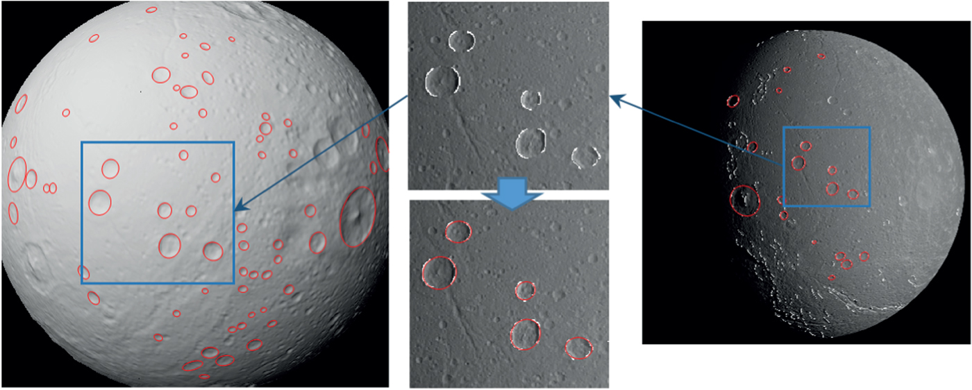
Figure 8. Crater map of Dione (Moon of Saturn) along with demonstrations of crater detection and ellipse fitting.
For each orbital image, crater models were projected onto the image using the true camera pose to yield true crater parameters, which were compared with the parameters of detected craters to determine the ellipse fitting error in crater detection.
The overall crater detection rate is 92%, which is consistent with state-of-the-art crater detection studies (Yu et al., Reference Yu, Cui and Tian2014; Cheng et al., Reference Cheng, Johnson and Matthies2005; Woicke et al., Reference Woicke, Moreno Gonzalez, El-Hajj, Mes, Henkel, Autar and Klavers2018). The detected craters were classified into two groups, namely the fine shape group and the irregular group. Table 1 shows the ellipse fitting error results (unit: pixel), where the crater centre position bias, semi-major and semi-minor axis length bias between detected craters and their counterparts in the crater map are calculated.
Table 1. Average fitting errors of crater rims (unit: pixel).

From Table 1 it can be seen that the ellipse fitting method for the fine-shape group yields an average bias of less than one pixel for three parameters, indicating a plausible ellipse fitting result. In comparison, the parameter biases in the irregular shape group are roughly three times bigger than those in the fine shape group. An important lesson was learned from this simulation, which is that the shape of the crater has an effect on navigation accuracy. To cope with this issue, one possible solution is to remove the craters with irregular shapes from the crater map, thereby guiding the crater matching to be carried out between craters with regular shapes.
4.2. Simulation of crater-based navigation method
A terrain landscape simulator was developed as a test bed for validating the proposed algorithm. An example of the simulated 3D terrain is presented in Figure 9; this simulator can generate craters with arbitrary size and shape. In this example case, four craters with different size and location were simulated. The Canny edge algorithm (Canny, Reference Canny1986) was adopted to detect the crater's edge, Figure 10 shows the rendered descent image of Figure 9 along with the crater edge detection results. The resolution of a rendered image was set to  $1024\times 1024$, and the field of view of the navigation camera was set to
  $44^{\circ}\times 44^{\circ}$.

Figure 9. Overview of a 3D terrain.

Figure 10. Generated image and edge detection results.
4.2.1. Case one: Three or more craters
The first simulation was carried under the condition where three or more craters were observed. Three non-overlapping crater edge curves were randomly generated in the field of view of the on board camera, the length of the semi-major and semi-minor axes were randomly selected in the range 0·5 km–2·5 km, and the maximum angle between the crater normal and the optical axis of the camera was set to 30°. The length of the crater edge was randomly selected to be in the range 10~100 pixels. Points on the crater edge had Gaussian-distributed noise added with a standard deviation of one pixel. The altitude of the lander varied between 10 km–100 km. At each altitude, a hundred Monte Carlo simulations were carried out using the proposed method. The means and standard deviation of position estimate error are presented in Figure 11.

Figure 11. Means and standard deviations of position estimate error under the condition of three or more craters observed.
As shown in Figure 11, the average positioning error and its standard deviation error tend to grow as the altitude of the lander increases, the minimum position estimate error is 0·258 km ± 0·227 km, which occurs at an altitude of 10 km; the maximum position estimate error is 0·945 km ± 0·593 km, which occurs at an altitude of 100 km. The trend of position estimate error using the Positioning method of the Crater Image Centre (PCCI) is the same as Positioning method based on the Edge of Crater (PEC), but the average position estimate error and the corresponding standard deviation are significantly higher than that with the PEC method. Simulation results indicate that when the optical axis of the navigation camera is not parallel to the normal of the crater, the deviation between the centre of the crater in the descent image and its true line of sight has a non-negligible effect on the pose estimation. Figure 12 shows the means and standard deviations of attitude estimate error results. Unlike the position estimation results, the overall trend of the attitude estimate error decreases as the altitude increases.

Figure 12. Means and standard deviations of attitude estimate error under the condition of three or more craters observed.
4.2.2. Case two: Two craters
The same simulation conditions were applied to the case where two craters were observed. The position and attitude error are shown in Figures 13 and 14, respectively.

Figure 13. Average positioning error and standard deviation of error with two craters.

Figure 14. Average attitude error and standard deviation of error with two craters.
As shown in Figures 13 and 14, the maximum average position estimate error is 0·107 km at altitude 100 km with a standard deviation of 0·203 km; the maximum average attitude estimate error is 0·173° at altitude 80 km with a standard deviation of 0·35°. The error of position estimate using two craters was even smaller than using three or more crater centres (PCCI method), which is mainly due to imposed constraints of the crater shape parameters.
4.2.3. Case three: Single/multiple craters and distributed EKF filter
Finally, the single crater-based navigation method along with other proposed methods was verified under the distributed EKF filter structure. Consider that the proposed method relies on the elliptical parameters of the detected edge (see Equation (3), parameters A~F), the standard deviations (std.) of the estimated error of the edge parameters is presented in Table 2. The std. errors were collected by extracting crater edges from several rendered descent images. Specifically, for each altitude, 128 rendered images were first used to detect the crater edges, and then the edge curve parameters’ errors were collected.
Table 2. Standard deviation of error in crater edge parameter estimation at different altitudes.

Results from Table 2 can serve as a reference to set the observation noise. Accordingly, the covariance of the measurement noise in the distributed EKF filter was set to:
 $$Q_{n}=\left[\matrix{ 2{\cdot}5\times 10^{-5} & 0 & 0 & 0 & 0 & 0 \cr 0 & 1{\cdot}5\times 10^{-4} & 0 & 0 &0 & 0 \cr 0 & 0 & 2{\cdot}5\times 10^{-5} & 0 & 0 & 0 \cr 0 & 0 & 0 & 1{\cdot}5\times 10^{-6} & 0 & 0 \cr 0 & 0 & 0 & 0 & 1{\cdot}5\times 10^{-6} & 0 \cr 0 & 0 & 0 & 0 & 0 & 1{\cdot}5\times 10^{-8} }\right]$$
A sub-EKF was constructed for each crater after obtaining its edge parameters A~F. The filter state includes the lander's three-axis position, velocity, angular velocity and lander attitude expressed by quaternions. If multiple craters were observed, the information was fused to couple all the sub-EKFs into a distributed EKF filter, which corresponds to Equations (25)~(29).
The same simulation parameter set-up in the first and second case was followed. To simplify the problem, the attitude of the lander was assumed to remain stable throughout the descent. Figures 15 and 16 show the time history of the lander pose estimation error along with the number of observed craters for one simulation trial. During the initial phase of the descent, the number of observed craters was three. The position and attitude errors of the lander quickly converged to 40 m and 0.05° at an altitude of 26 km. After the lander reached 26 km, the on board camera can only observe one crater, causing the attitude estimation error to slightly increase as the landing proceeds. This is because the solar illumination direction, as a complementary observation to estimate the lander's pose, is much less accurate than the crater edge estimation. Nevertheless, the crater edge-based navigation method is still effective in suppressing the accumulated errors.

Figure 15. Position estimate error of the crater edge-based distributed EKF filter.

Figure 16. Attitude estimate error of the crater edge-based distributed EKF filter.
A total number of thirty sets of simulated terrains were generated for the Monte Carlo (MC) simulation. In each MC trial, the initial lander position, velocity, attitude and angular velocity were assumed to be mixed with zero-mean Gaussian distributed noise, with standard deviations of 4 km, 5 m/s, 25 deg and 5°/s, respectively. The standard deviation of the tilt angle noise for the solar illumination direction is 10°. Figures 17 and 18 show the average position and attitude estimate error collected from the MC simulation. Along with the estimated error, the average number of craters which lie in the camera's field of view is shown in these two figures. It can be seen that the average position and attitude estimation tend to converge when at least two craters are observed. When the average number of observed craters is less than two, the pose estimated error grows slowly as the landing proceeds. When the lander reaches the final recorded altitude at 10 km, the average position estimate error is less than 200 m, and the average attitude estimate error is less than 1°, demonstrating the effectiveness of the proposed crater edge-based navigation approach.

Figure 17. Average lander position estimated error of the MC simulation.

Figure 18. Average lander attitude estimated error of the MC simulation.
5. CONCLUSION
This paper presents a novel method for autonomous navigation during an extra-terrestrial body landing mission. The proposed method establishes crater edge and solar illumination direction-based measurement models and incorporates the measurement models into a distributed EKF filter to achieve crater-aided inertial navigation. Monte Carlo Simulations show that the proposed approach performs better than the state-of-the-art crater centre-based algorithms and is able to give a plausible estimate result when only one crater is observed, demonstrating its superiority in terms of navigation flexibility.
Future work will include a more credible semi-physical test of the proposed algorithm, where the effect of lighting conditions, crater shape, and other factors on navigational performance will be investigated.
ACKNOWLEDGEMENTS
The work described in this paper was supported by the National Natural Science Foundation of China (Grant No. 61503102, 61673057 and 61701225), the Opening Grant from the Key Laboratory of Space Utilization, Chinese Academy of Sciences (Grant No. LSU-KJTS-2017-01). The authors fully appreciate their financial supports.


