


1 Introduction
Many real-life systems of engineering and physical interest are governed by nonlinear wave equations: nonlinear circuits, nonlinear optics, ocean surface waves, planetary waves in the atmosphere, etc. (Kraichnan Reference Kraichnan1967; Rewienski & White Reference Rewienski and White2003; Lynch Reference Lynch2009; Kibler et al. Reference Kibler, Fatome, Finot, Millot, Dias, Genty, Akhmediev and Dudley2010). One of the hallmarks of nonlinear dynamics is the transfer of energy across scales, so modelling and understanding energy transfer in nonlinear systems is key to predicting and harnessing extreme events in these physical systems. One such system, the Charney–Hasagawa–Mima (CHM) equation (which will be the focus of this paper) is a nonlinear dispersive partial differential equation (PDE) which can be used to describe Rossby waves in the atmosphere and drift waves in plasmas.
One approach to understanding how nonlinear systems behave is model reduction, where one simplifies the system to a point that is easier to study mathematically, while leaving enough complexity in the system so that the phenomena under scrutiny remain in the reduced model. A common method is spectral truncation, where one considers only a small set of interacting modes in Fourier space. Often these reduced models are studied from a dynamical systems point of view where interesting feedback mechanisms have been proposed (Waleffe Reference Waleffe1997): as more complex models are considered, these mechanisms have survived in the form of periodic orbits. Other dynamical systems approaches in fluid mechanics include studying shell models (Biferale Reference Biferale2003; Mailybaev Reference Mailybaev2013), and the search and classification of unstable periodic orbits in higher-dimensional systems (Kawahara & Kida Reference Kawahara and Kida2001; Lucas & Kerswell Reference Lucas and Kerswell2015, Reference Lucas and Kerswell2017).
A useful method for analysing models that are based on dynamical systems of any dimension is the method of normal forms. The normal form transformation of a dynamical system is often described as a nonlinear transformation of coordinates in which the dynamical system takes its ‘simplest’ form (Wiggins Reference Wiggins2003). There is a certain amount of freedom one can take with the form of the transformation; however, its usual manifestation involves eliminating as many non-resonant terms as possible from the evolution equations. This method dates back to Poincaré, and was developed for the  $N$-body problem in celestial mechanics. Analytic study of convergence of these normal form transformations is quite difficult and often concerns with whether the series will converge at all (Perez-Marco Reference Perez-Marco2003; Bruno, Hovingh & Coleman Reference Bruno, Hovingh and Coleman2011; Krikorian Reference Krikorian2019). The study of the region of convergence is comparatively rare; however, it is still of interest in nonlinear wave systems:
(i) For example, in the Fermi–Pasta–Ulam–Tsingou system the normal form transformation is important in establishing the applicability of the Kolmogorov–Arnold–Moser theorem. In the weakly nonlinear limit the normal form transformation of the Hamiltonian calculated and truncated to fourth order can be shown to be integrable, and the full nonlinear system can be considered to be a small perturbation to this integrable system at small amplitudes. However, as explained by Rink (Reference Rink2006), no study of convergence has been performed to date.
(ii) As a second example, in the case of surface gravity water waves propagating in one spatial dimension in a basin of infinite depth, it is well known that the formal truncation of the expansion of the Hamiltonian up to and including quartet interactions leads to an integrable system (Dyachenko & Zakharov Reference Dyachenko and Zakharov1994; Craig & Worfolk Reference Craig and Worfolk1995). However, it took 24 years to find a rigorous proof that the flow stemming from the original Hamiltonian could be well approximated by the flow stemming from this formal truncation (Berti, Feola & Pusateri Reference Berti, Feola and Pusateri2018). This rigorous proof not only provided a quantitative assessment of the boundedness of the error (quintet terms): more interestingly, it provided a remarkable long-time existence result (
 $T_{\unicode[STIX]{x1D716}}\sim \unicode[STIX]{x1D716}^{-3}$ as opposed to the natural $T_{\unicode[STIX]{x1D716}}\sim \unicode[STIX]{x1D716}^{-2}$ that would be expected from wave turbulence phenomenology), where $T_{\unicode[STIX]{x1D716}}$ is the nonlinear time scale and $\unicode[STIX]{x1D716}$ is proportional to the wave amplitudes for the solution stemming from the full Hamiltonian. Thus, the normal form transformation provides a quantifiably useful and accurate approximation in the case of weak nonlinearity, but we do not know the level of nonlinearity at which the transformation breaks down.


Despite the lack of rigorous convergence results, one of the most fruitful approaches to studying nonlinear wave equations has been the theory of wave turbulence (Nazarenko Reference Nazarenko2011), which uses normal form transformations to eliminate non-resonant interactions from the system. In the usual formulation of wave turbulence, the limits of both small amplitudes and large domain are considered. The small amplitudes allow for the non-resonant terms to be eliminated as the non-zero linear frequencies of oscillation in the system are much faster than the nonlinear frequencies, and the large box limit allows for a continuum of wavenumbers in the system. For some systems these limits are a good approximation. An example of this is gravity water waves, where the steepness of the waves is typically small and a large domain (compared to the relevant wavelengths) makes physical sense. Normal form transformations have been very effective in this case: these transformations were originally calculated by Krasitskii for a general dispersive and weakly nonlinear system, and were applied to water waves by Zakharov and Dyachenko (Krasitskii Reference Krasitskii1990; Dyachenko, Lvov & Zakharov Reference Dyachenko, Lvov and Zakharov1995).
However, all physical systems have finite amplitude and all numerical simulations must be performed on a finite domain, and moreover there are many nonlinear wave systems where the large box or weak amplitude approximations are not good assumptions, so studying the behaviour of systems when these two assumptions are relaxed is important. Once finite amplitudes are introduced it is necessary to understand how and where the normal form transformation converges: we cannot truncate higher-order terms immediately without properly assessing the truncation error, which involves quantifying the rate of convergence. Also, certain phenomena are observed at finite amplitudes only, such as precession resonance (Bustamante, Quinn & Lucas Reference Bustamante, Quinn and Lucas2014), which manifests itself in PDE systems as transient bursts of energy transfers between modes.
In this paper we consider a reduced model consisting of a Galerkin truncation of the CHM equation to four Fourier modes, and ask the question: Can precession resonance be described by the normal form variables of wave turbulence theory? The answer is no, and we provide abundant quantitative evidence. In § 2 we describe the CHM equation and how precession resonance can be observed at finite Fourier amplitudes. We then take a low-dimensional Galerkin truncation that demonstrates precession resonance and we investigate how the resonance manifests itself in state space. In § 3 we begin our investigation of the possible manifestation of precession resonance in normal form coordinates. First, in § 3.1 we define the normal form transformation and detail how it is developed out of the evolution equations of our Galerkin truncated system. The usual wave turbulence approach involves calculating the normal form transformation from a Hamiltonian; however, in the case of the CHM equation it is more natural to compute it directly from the evolution equations. From there we calculate the transformation eliminating up to non-resonant 4-wave interactions and probing the mechanism in a similar fashion as was done in § 2. We find that there is a large discrepancy between the evolution of the original equations and the transformed equations, suggesting that the normal form transformation may not be convergent. Thus, in § 3.2 we quantify the convergence of the normal form transformation at finite amplitudes. We obtain robust numerical evidence of convergence over a finite region of wave amplitudes, and we estimate numerically the boundary of this region, i.e. the amplitudes at which the transformation begins to diverge. We find that this boundary is very close to the set of initial conditions that lead to precession resonance, and we assess this closeness quantitatively. Finally, we provide concluding remarks in § 4.
2 Precession resonance in the CHM equation
2.1 The CHM equation and the weakly nonlinear limit
Consider the Charney–Hasagawa–Mima equation, a PDE model for Rossby waves in the atmosphere as well as drift waves in plasmas,
 $$\begin{eqnarray}(\unicode[STIX]{x1D6FB}^{2}-F)\frac{\unicode[STIX]{x2202}\unicode[STIX]{x1D713}}{\unicode[STIX]{x2202}t}+\unicode[STIX]{x1D6FD}\frac{\unicode[STIX]{x2202}\unicode[STIX]{x1D713}}{\unicode[STIX]{x2202}x}+\frac{\unicode[STIX]{x2202}\unicode[STIX]{x1D713}}{\unicode[STIX]{x2202}x}\frac{\unicode[STIX]{x2202}\unicode[STIX]{x1D6FB}^{2}\unicode[STIX]{x1D713}}{\unicode[STIX]{x2202}y}-\frac{\unicode[STIX]{x2202}\unicode[STIX]{x1D713}}{\unicode[STIX]{x2202}y}\frac{\unicode[STIX]{x2202}\unicode[STIX]{x1D6FB}^{2}\unicode[STIX]{x1D713}}{\unicode[STIX]{x2202}x}=0,\end{eqnarray}$$
 where  $\unicode[STIX]{x1D713}$ is the streamfunction of a geophysical flow and
  $F\geqslant 0$ is the Rossby deformation radius. Assuming periodic boundary conditions
  $\boldsymbol{x}\in [\!0,2\unicode[STIX]{x03C0}\!)^{2}$, we can decompose the equation into its Fourier components
  $A_{\boldsymbol{k}}$ defined by
  $\unicode[STIX]{x1D713}(\boldsymbol{x},t)=\sum _{\boldsymbol{k}\in \mathbb{Z}^{2}}A_{\boldsymbol{k}}(t)\text{e}^{\text{i}\boldsymbol{k}\boldsymbol{\cdot }\boldsymbol{x}}+\text{c.c.}$, which leads to
 $$\begin{eqnarray}{\dot{A}}_{\boldsymbol{k}}+\text{i}\unicode[STIX]{x1D714}_{\boldsymbol{k}}A_{\boldsymbol{k}}=\frac{1}{2}\mathop{\sum }_{\boldsymbol{k}_{1}\boldsymbol{k}_{2}\in \mathbb{Z}}Z_{\boldsymbol{k}_{1}\boldsymbol{k}_{2}}^{\boldsymbol{ k}}\unicode[STIX]{x1D6FF}_{\boldsymbol{k}_{1}+\boldsymbol{k}_{2}-\boldsymbol{k}}A_{\boldsymbol{k}_{1}}A_{\boldsymbol{k}_{2}},\quad \boldsymbol{k}\in \mathbb{Z}^{2},\end{eqnarray}$$
where
 $$\begin{eqnarray}Z_{\boldsymbol{k}_{1}\boldsymbol{k}_{2}}^{\boldsymbol{ k}}=\frac{(k_{1x}k_{2y}-k_{1y}k_{2x})(|\boldsymbol{k}_{1}|^{2}-|\boldsymbol{k}_{2}|^{2})}{|\boldsymbol{k}|^{2}+F},\quad \unicode[STIX]{x1D714}_{\boldsymbol{k}}=\frac{-\unicode[STIX]{x1D6FD}k_{x}}{|\boldsymbol{k}|^{2}+F}.\end{eqnarray}$$
 Due to the Kronecker delta on the right-hand side of (2.2), we can see that the only nonlinear contributions to mode  $A_{\boldsymbol{k}}$ come from modes
  $A_{\boldsymbol{k}_{1}}$ and
  $A_{\boldsymbol{k}_{2}}$ whenever
  $\boldsymbol{k}=\boldsymbol{k}_{1}+\boldsymbol{k}_{2}$. These are known as triad interactions (Kraichnan Reference Kraichnan1967).
In the limit of small amplitudes, the evolution of  $A_{\boldsymbol{k}}$ in (2.2) is dominated by the linear dispersion relation
  $\unicode[STIX]{x1D714}_{\boldsymbol{k}}$. These waves are known as Rossby waves. To see how the nonlinear term contributes to the dynamics we perform a change of variable
  $a_{\boldsymbol{k}}(t)=\text{e}^{\text{i}\unicode[STIX]{x1D714}_{\boldsymbol{k}}t}A_{\boldsymbol{ k}}(t)$ to obtain our equations in the so-called interaction representation,
 $$\begin{eqnarray}{\dot{a}}_{\boldsymbol{k}}=\frac{1}{2}\mathop{\sum }_{\boldsymbol{k}_{1},\boldsymbol{k}_{2}\in \mathbb{Z}^{2}}Z_{\boldsymbol{k}_{1}\boldsymbol{k}_{2}}^{\boldsymbol{ k}}\unicode[STIX]{x1D6FF}_{\boldsymbol{k}_{1}+\boldsymbol{k}_{2}-\boldsymbol{k}}a_{\boldsymbol{k}_{1}}a_{\boldsymbol{k}_{2}}\text{e}^{-\text{i}\unicode[STIX]{x1D714}_{\boldsymbol{k}_{1}\boldsymbol{k}_{2}}^{\boldsymbol{k}}t},\end{eqnarray}$$
 where  $\unicode[STIX]{x1D714}_{\boldsymbol{k}_{1}\boldsymbol{k}_{2}}^{\boldsymbol{k}}=\unicode[STIX]{x1D714}_{\boldsymbol{ k}_{1}}+\unicode[STIX]{x1D714}_{\boldsymbol{k}_{2}}-\unicode[STIX]{x1D714}_{\boldsymbol{k}}$.
Inspecting (2.4) we can see that when the amplitudes  $a_{\boldsymbol{k}}$ are sufficiently small (so-called weakly nonlinear limit) their evolution becomes significantly slower than the linear oscillations. This can be seen if we replace
  $a_{\boldsymbol{k}}\rightarrow \unicode[STIX]{x1D716}a_{\boldsymbol{k}}$. This gives us a factor of
  $\unicode[STIX]{x1D716}$ in front of the terms on the right-hand side of (2.4). If we make a change of variables
  $\unicode[STIX]{x1D70F}=\unicode[STIX]{x1D716}t$, then we have
 $$\begin{eqnarray}\frac{\text{d}a_{\boldsymbol{k}}}{\text{d}\unicode[STIX]{x1D70F}}=\frac{1}{2}\mathop{\sum }_{\boldsymbol{k}_{1},\boldsymbol{k}_{2}\in \mathbb{Z}^{2}}Z_{\boldsymbol{k}_{1}\boldsymbol{k}_{2}}^{\boldsymbol{ k}}\unicode[STIX]{x1D6FF}_{\boldsymbol{k}_{1}+\boldsymbol{k}_{2}-\boldsymbol{k}}a_{\boldsymbol{k}_{1}}a_{\boldsymbol{k}_{2}}\text{e}^{-\text{i}\unicode[STIX]{x1D714}_{\boldsymbol{k}_{1}\boldsymbol{k}_{2}}^{\boldsymbol{k}}\unicode[STIX]{x1D70F}/\unicode[STIX]{x1D716}}.\end{eqnarray}$$
 Equation (2.5) shows that as we decrease  $\unicode[STIX]{x1D716}$, the time scale separation between our linear and nonlinear oscillations grows. This implies that at these small amplitudes, the fast oscillations of
  $\text{e}^{-\text{i}\unicode[STIX]{x1D714}_{\boldsymbol{k}_{1}\boldsymbol{k}_{2}}^{\boldsymbol{k}}t}$ average out to zero for
  $\unicode[STIX]{x1D714}_{\boldsymbol{k}_{1}\boldsymbol{k}_{2}}^{\boldsymbol{k}}\neq 0$, meaning that the only meaningful triad interactions occur when
  $\unicode[STIX]{x1D714}_{\boldsymbol{k}}=\unicode[STIX]{x1D714}_{\boldsymbol{k}_{1}}+\unicode[STIX]{x1D714}_{\boldsymbol{k}_{2}}$, the so-called resonant condition. Thus in the weakly nonlinear limit the non-resonant triad interactions (defined by the inequality
  $\unicode[STIX]{x1D714}_{\boldsymbol{k}_{1}\boldsymbol{k}_{2}}^{\boldsymbol{k}}\neq 0$) do not contribute to the long-time dynamics of the system. In the classical theory of wave turbulence a nonlinear near-identity change of coordinates is performed to eliminate these non-resonant interactions from the equations, in what is often referred to as a normal form transformation (Nazarenko Reference Nazarenko2011).
2.2 Precession resonance
To understand precession resonance we must first consider the equations in phase-amplitude form, where
 $$\begin{eqnarray}A_{\boldsymbol{k}}=n_{\boldsymbol{k}}\text{e}^{\text{i}\unicode[STIX]{x1D719}_{\boldsymbol{k}}},\end{eqnarray}$$
 where  $n_{\boldsymbol{k}}\in [0,\infty )$ and
  $\unicode[STIX]{x1D719}_{\boldsymbol{k}}\in [0,2\unicode[STIX]{x03C0})$. To allow for phase precessions (Bustamante et al. Reference Bustamante, Quinn and Lucas2014) (also known as phase-slips (Gandhi, Knobloch & Beaume Reference Gandhi, Knobloch and Beaume2015)) we will consider
  $\unicode[STIX]{x1D719}_{\boldsymbol{k}}\in (-\infty ,\infty )$. Upon transforming our evolution equations to phase-amplitude form we will see that due to the triad interactions the Fourier phases do not appear isolated. Rather, they appear in triad combinations
  $\unicode[STIX]{x1D711}_{\boldsymbol{k}_{1}\boldsymbol{k}_{2}}^{\boldsymbol{k}}=\unicode[STIX]{x1D719}_{\boldsymbol{ k}_{1}}+\unicode[STIX]{x1D719}_{\boldsymbol{k}_{2}}-\unicode[STIX]{x1D719}_{\boldsymbol{k}}$ known as Fourier triad phases, where
  $\boldsymbol{k}_{1}+\boldsymbol{k}_{2}=\boldsymbol{k}$. Our equations take the form
 $$\begin{eqnarray}\displaystyle & \displaystyle {\dot{n}}_{\boldsymbol{k}}=\mathop{\sum }_{\boldsymbol{k}_{1}\boldsymbol{k}_{2}}Z_{\boldsymbol{k}_{1}\boldsymbol{k}_{2}}^{\boldsymbol{k}}\unicode[STIX]{x1D6FF}_{\boldsymbol{k}_{1}+\boldsymbol{k}_{2}-\boldsymbol{k}}n_{\boldsymbol{k}_{1}}n_{\boldsymbol{k}_{2}}\cos \unicode[STIX]{x1D711}_{\boldsymbol{k}_{1}\boldsymbol{k}_{2}}^{\boldsymbol{k}}, & \displaystyle\end{eqnarray}$$
 $$\begin{eqnarray}\displaystyle & \displaystyle \dot{\unicode[STIX]{x1D711}}_{\boldsymbol{k}_{1}\boldsymbol{k}_{2}}^{\boldsymbol{k}_{3}}=\sin \unicode[STIX]{x1D711}_{\boldsymbol{ k}_{1}\boldsymbol{k}_{2}}^{\boldsymbol{k}_{3}}n_{\boldsymbol{ k}_{3}}n_{\boldsymbol{k}_{1}}n_{\boldsymbol{k}_{2}}\left(\frac{Z_{\boldsymbol{k}_{2}\boldsymbol{k}_{3}}^{\boldsymbol{k}_{1}}}{n_{\boldsymbol{k}_{1}}^{2}}+\frac{Z_{\boldsymbol{k}_{3}\boldsymbol{k}_{1}}^{\boldsymbol{k}_{2}}}{n_{\boldsymbol{k}_{2}}^{2}}-\frac{Z_{\boldsymbol{k}_{1}\boldsymbol{k}_{2}}^{\boldsymbol{k}_{3}}}{n_{\boldsymbol{k}_{3}}^{2}}\right)-\unicode[STIX]{x1D714}_{\boldsymbol{k}_{1}\boldsymbol{k}_{2}}^{\boldsymbol{k}_{3}}+\text{NNTT}_{\boldsymbol{ k}_{1}\boldsymbol{k}_{2}}^{\boldsymbol{k}_{3}}. & \displaystyle\end{eqnarray}$$
 The terms  $\text{NNTT}_{\boldsymbol{k}_{1}\boldsymbol{k}_{2}}^{\boldsymbol{k}_{3}}$ are the nearest neighbouring triad terms connected to the triad
  $\boldsymbol{k}_{1}+\boldsymbol{k}_{2}=\boldsymbol{k}_{3}$. To illustrate the form this term takes, the neighbouring terms connected to
  $\boldsymbol{k}_{1}$ take the form
 $$\begin{eqnarray}\text{NNTT}_{\boldsymbol{k}_{1}\boldsymbol{k}_{2}}^{\boldsymbol{ k}_{3}}=\mathop{\sum }_{\boldsymbol{k}_{4},\boldsymbol{k}_{5}}\sin \unicode[STIX]{x1D711}_{\boldsymbol{k}_{4}\boldsymbol{k}_{5}}^{\boldsymbol{ k}_{1}}n_{\boldsymbol{k}_{1}}n_{\boldsymbol{k}_{4}}n_{\boldsymbol{k}_{5}}\frac{Z_{\boldsymbol{k}_{4}\boldsymbol{k}_{5}}^{\boldsymbol{k}_{1}}}{n_{\boldsymbol{k}_{1}}^{2}}\unicode[STIX]{x1D6FF}_{\boldsymbol{k}_{4}+\boldsymbol{k}_{5}-\boldsymbol{k}_{1}}+\cdots \,,\end{eqnarray}$$
 with similar terms for  $\boldsymbol{k}_{2}$ and
  $\boldsymbol{k}_{3}$ (see the full form in Bustamante et al. (Reference Bustamante, Quinn and Lucas2014)). We define the precession frequency as the local average
  $\unicode[STIX]{x1D6FA}_{\boldsymbol{k}_{1}\boldsymbol{k}_{2}}^{\boldsymbol{k}}(t)\equiv (1/T)\int _{t}^{t+T}\dot{\unicode[STIX]{x1D711}}_{\boldsymbol{ k}_{1}\boldsymbol{k}_{2}}^{\boldsymbol{k}}(t^{\prime })\,\text{d}t^{\prime }$, where
  $T$ is a suitably chosen time scale, larger than the typical nonlinear time scale. Geometrically, this corresponds to the frequency at which
  $\unicode[STIX]{x1D711}_{\boldsymbol{k}_{1}\boldsymbol{k}_{2}}^{\boldsymbol{k}}$ winds around the origin. In the weakly nonlinear case this precession frequency is dominated by the linear term, i.e.
  $\unicode[STIX]{x1D6FA}_{12}^{3}\rightarrow -\unicode[STIX]{x1D714}_{12}^{3}$ as our amplitudes become small. However, if we extend our system beyond the weakly nonlinear limit and start taking into account finite amplitudes, the nonlinear terms begin to contribute to the dynamics and in particular to the precession frequency.
Looking at the right-hand side of (2.7), we can see that if the characteristic nonlinear frequency of  $n_{\boldsymbol{k}_{1}}n_{\boldsymbol{k}_{2}}$ is commensurate with the precession frequency
  $\unicode[STIX]{x1D6FA}_{\boldsymbol{k}_{1}\boldsymbol{k}_{2}}^{\boldsymbol{k}}$ we then get a zero mode in the evolution equation of
  $n_{\boldsymbol{k}}$ which leads to sustained growth. The strongest manifestation of this is the zero harmonic resonance, where
  $\unicode[STIX]{x1D6FA}_{\boldsymbol{k}_{1}\boldsymbol{k}_{2}}^{\boldsymbol{k}}=0$. It follows from (2.7) that if this condition is satisfied then we obtain strong growth in mode
  $A_{\boldsymbol{k}}$. One of the remarkable things about precession resonance is that we can always trigger this resonance simply by rescaling the amplitudes of the initial conditions by a constant
  $\unicode[STIX]{x1D6FC}$. As we increase
  $\unicode[STIX]{x1D6FC}$, the nonlinear contributions to (2.8) can become of the order of the linear part
  $\unicode[STIX]{x1D714}_{\boldsymbol{k}_{1}\boldsymbol{k}_{2}}^{\boldsymbol{k}_{3}}$ and cancel, resulting in
  $\unicode[STIX]{x1D6FA}_{\boldsymbol{k}_{1}\boldsymbol{k}_{2}}^{\boldsymbol{k}}=0$.
As the precession frequency of a triad depends on many terms of the system, its value changes dynamically as the system evolves. In full PDE systems precession resonance manifests itself as transient bursts of energy transfers between modes interacting via non-resonant triads. These bursts occur when the precession frequency becomes commensurate with the nonlinear frequency of oscillations of the system over a finite time  $T$. In a Galerkin truncated system, precession frequency strongly depends on the number of truncated modes if the number of modes is small. If we take the limit of the number of modes to infinity, the precession frequency converges to the value corresponding to the full PDE.
2.3 Model reduction
The simplest manifestation of precession resonance for the CHM model occurs in a Galerkin truncation to four Fourier modes. Our system is composed of a resonant triad joined to a fourth mode by two modes via a non-resonant triad (see figure 1). Putting a small parameter  $\unicode[STIX]{x1D716}$ in front of the second triad interaction coefficients allows us to match our results with the reduced model in (Bustamante et al. Reference Bustamante, Quinn and Lucas2014). It also allows us to focus our attention on the effect of precession resonance on the energy transfers to one particular mode, which we choose to be
  $A_{4}$.

Figure 1. (a) Schematic representation of our reduced system. (b) Plots of the normalised function of time  $|A_{4}(t)|/\unicode[STIX]{x1D6FC}$, for initial conditions from (2.11) in terms of the scaling parameter
  $\unicode[STIX]{x1D6FC}$ taking different values as in the legend. The resonant scaling value at
  $\unicode[STIX]{x1D6FC}=\unicode[STIX]{x1D6FC}_{r}\approx 2.114137$ shows a strong energy transfer to
  $A_{4}$.
Our equations are
 $$\begin{eqnarray}\left.\begin{array}{@{}c@{}}{\dot{A}}_{1}=-\text{i}\unicode[STIX]{x1D714}_{1}A_{1}+z_{1}A_{2}^{\ast }A_{3}\\ {\dot{A}}_{2}=-\text{i}\unicode[STIX]{x1D714}_{2}A_{2}+z_{2}A_{1}^{\ast }A_{3}+\unicode[STIX]{x1D716}s_{2}A_{3}^{\ast }A_{4}\\ {\dot{A}}_{3}=-\text{i}\unicode[STIX]{x1D714}_{3}A_{3}+z_{3}A_{1}A_{2}+\unicode[STIX]{x1D716}s_{3}A_{2}^{\ast }A_{4}\\ {\dot{A}}_{4}=-\text{i}\unicode[STIX]{x1D714}_{4}A_{4}+\unicode[STIX]{x1D716}s_{4}A_{2}A_{3}\\ \unicode[STIX]{x1D714}_{3}=\unicode[STIX]{x1D714}_{1}+\unicode[STIX]{x1D714}_{2},\quad \unicode[STIX]{x1D714}_{4}\neq \unicode[STIX]{x1D714}_{2}+\unicode[STIX]{x1D714}_{3},\end{array}\right\}\end{eqnarray}$$
 our parameters being  $F=1$,
  $\unicode[STIX]{x1D6FD}=10$,
  $\unicode[STIX]{x1D716}=0.01$,
  $\boldsymbol{k}_{1}=(1,-4)$,
  $\boldsymbol{k}_{2}=(1,2)$,
  $\boldsymbol{k}_{3}=(2,-2)$ and
  $\boldsymbol{k}_{4}=(3,0)$. Using the formulae for the dispersion relation and interaction coefficients in (2.3) we calculate
  $\unicode[STIX]{x1D714}_{1}=-5/9$,
  $\unicode[STIX]{x1D714}_{2}=-5/3$,
  $\unicode[STIX]{x1D714}_{3}=-20/9$,
  $\unicode[STIX]{x1D714}_{4}=-3$,
  $z_{1}=-1$,
  $z_{2}=-9$,
  $z_{3}=8$,
  $s_{2}=1$,
  $s_{3}=-8/3$ and
  $s_{4}=-9/5$. This gives us
  $\unicode[STIX]{x1D714}_{12}^{3}=0$ and
  $\unicode[STIX]{x1D714}_{23}^{4}=-8/9$.
In order to search for precession resonance we will explore a set of initial conditions for our variables  $A_{j},j=1,\ldots ,4$, of the form
 $$\begin{eqnarray}\left.\begin{array}{@{}c@{}}\displaystyle A_{1}(0)=(0.0245+0.001\text{i})\unicode[STIX]{x1D6FC},\quad A_{2}(0)=(0.01+0.01\text{i})\unicode[STIX]{x1D6FC},\\ \displaystyle A_{3}(0)=0.02236\unicode[STIX]{x1D6FC},\quad A_{4}(0)=0,\end{array}\right\}\end{eqnarray}$$
 where, except for  $A_{4}(0)$, the numerical coefficients were randomly chosen, and
  $\unicode[STIX]{x1D6FC}$ is our real scaling parameter. The size of the numerical coefficients was chosen so that the linear terms in the equations dominate over the nonlinear terms when
  $|\unicode[STIX]{x1D6FC}|\ll 1$. In figure 1 on the right we observe that, as we get close to the exact scaling value (
 $\unicode[STIX]{x1D6FC}_{r}\approx 2.114137$) for the initial condition (2.11) which leads to precession resonance, our energy transfer to mode
  $A_{4}$ greatly increases. As we scale past that value, the energy transfer efficiency becomes weak again.
The choice of initial conditions with  $A_{4}(0)=0$ is for visualisation purposes as well as for maximising the effect of precession resonance to this mode. Precession resonance can occur for any arbitrary initial condition (see the study shown in figure 4a). However, a particularly interesting facet of precession resonance is the prospect of energy leaking to modes which start off with no energy and are not part of any resonant triads.
This phenomenon was described and studied in Bustamante et al. (Reference Bustamante, Quinn and Lucas2014). In this document we wish to better understand the geometric structure of the resonance in state space. We also wish to study the resonance in normal form coordinates used in wave turbulence theory to see if the resonance can manifest itself in the dynamics for the normal form coordinates.

Figure 2. For  $\unicode[STIX]{x1D6FC}\approx \unicode[STIX]{x1D6FC}_{r}\pm 10^{-6}$ saddle-node-like behaviour can be seen around the trajectory associated with precession resonance.
2.4 Invariant manifolds
For near resonant values of our scaling parameter  $\unicode[STIX]{x1D6FC}$, figure 2 shows saddle-node-like behaviour. This suggests a dynamical systems point of view whereby resonant trajectories in the reduced model could correspond to invariant manifolds such as critical points or periodic orbits in state space.
Figure 3 shows that, letting this system evolve for a long time, the resonance corresponds to a trajectory that gets close to a periodic orbit in state space and remains close for a while to then separate from it. Motion around the periodic orbit corresponds to the plateau seen in (a) from  $t=2000$ to
  $t=6000$. The bump around
  $t=7000$ is the orbit being ejected out the unstable manifold.

Figure 3. (a) Evolution of the slow dynamics of the system. The fast small oscillations corresponding to motion around the periodic orbit are not seen here. For  $\unicode[STIX]{x1D6FC}\approx \unicode[STIX]{x1D6FC}_{r}$,
  $A_{4}$ approaches a particular value. After a time it is ejected along an unstable manifold. (b) Zooming into a projection of the trajectory onto
  $|A_{4}|$,
  $\unicode[STIX]{x1D711}_{12}^{3}$ and
  $\unicode[STIX]{x1D711}_{23}^{4}$, we can see that the orbit approaches a periodic orbit.
To gain more insight into the geometric structure of this resonance, we consider how these manifolds manifest themselves in the state space. First, let us count the number of degrees of freedom. Equations (2.10) represent 4 complex equations for 4 complex variables. However, in terms of amplitude-phase representation, the phases appear only in two triad combinations so we can reduce the state space to 6 dynamical variables. Second, we have two conserved quantities, energy and enstrophy, defined as
 $$\begin{eqnarray}\left.\begin{array}{@{}c@{}}\displaystyle E=\mathop{\sum }_{i=1}^{4}(|\boldsymbol{k}_{i}|^{2}+F)|A_{i}|^{2},\\ \displaystyle {\mathcal{E}}=\mathop{\sum }_{i=1}^{4}|\boldsymbol{k}_{i}|^{2}(|\boldsymbol{k}_{i}|^{2}+F)|A_{i}|^{2},\end{array}\right\}\end{eqnarray}$$
which further reduces the dimension of the system by 2 units, leading to an effective four-dimensional system.
In § 2.3 we searched for resonances by re-scaling the initial conditions by a constant. While this shows how simple it is to find these resonances, it does not shed any light on the structure of the periodic orbits in state space. This prompts us to search for resonances contained in the invariant manifolds corresponding to fixed energy and enstrophy.
To perform this search of resonances constrained to fixed energy and enstrophy, we first proceed using the same re-scaling technique as before with  $\unicode[STIX]{x1D6FC}$ until we trigger a resonance. For the same initial conditions we used in § 2 we found that resonance occurred at
  $\unicode[STIX]{x1D6FC}_{r}\approx 2.114137$ giving resonant initial conditions to be
  $\boldsymbol{A}=(A_{1},A_{2},A_{3},A_{4})^{\text{T}}\approx (0.0518+0.0021\text{i},0.0211+0.0211\text{i},0.0472,0)^{\text{T}}$.
From these initial values we can now calculate the values for energy  $E=0.0738$ and enstrophy
  ${\mathcal{E}}=1.0097$ from (2.12). We will fix these values and perform a systematic search for resonances within the intersection of the manifolds
  $E=0.0738$ and
  ${\mathcal{E}}=1.0097$. To start, choose as initial condition
  $|A_{4\,new}|=|A_{4\,old}|+\unicode[STIX]{x1D6FF}$ where
  $\unicode[STIX]{x1D6FF}$ is a small positive number. We now vary the initial
  $|A_{1}|$, solving for
  $|A_{2}|$ and
  $|A_{3}|$ to make sure
  $E$ and
  ${\mathcal{E}}$ are unchanged, until a new resonance point is found. Throughout these searches we keep the initial complex phases unchanged. It was found that changing the complex phases still lead to a periodic orbit that could already be found using our current method, it would just shift the initial condition to another location along the orbit. As for the phase of the initial
  $A_{4}$, although our first initial value was
  $A_{4}=0$ and so
  $\arg (A_{4})$ was undefined, we have picked an arbitrary value for
  $\arg (A_{4})$ when
  $A_{4}\neq 0$ (in our case we chose
  $\arg (A_{4})=0$). The systematic search produces a continuous curve representing the points of resonance as can be seen in figure 4(a).

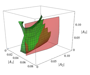
Figure 4. (a) A curve of initial values for  $|A_{1}|$ and
  $|A_{4}|$ on the same invariant energy and enstrophy manifolds that lead to precession resonance. The points correspond to the periodic orbits plotted in (b), in the sense that the initial condition implied by each point belongs to the stable manifold of the corresponding periodic orbit. (b) A set of periodic orbits associated with precession resonance on the same invariant manifolds. The orbits from right to left correspond to the points from right to left in (a).
Figure 4(b) shows the periodic orbits corresponding to some resonance points chosen along the curve in figure 4(a). So the resonant curve corresponds to a one-parameter family of periodic orbits. It is evident that two directions in state space have zero Lyapunov exponent: the direction along the periodic-orbit time evolution and the direction that connects the different periodic orbits. Since our system has 4 degrees of freedom and we already need to have a stable and an unstable manifold to reach the periodic orbits, we conclude that we can determine the structure and dimensions of all relevant manifolds in state space. We have a one-dimensional stable manifold, a one-dimensional unstable manifold and two neutral directions induced by the one-dimensional time evolution along the periodic orbits and the one-dimensional direction along which the periodic orbits are ordered. Moreover, from the fact that the original system is volume preserving, the Lyapunov exponents of the stable and unstable manifolds are  $-\unicode[STIX]{x1D6EC}$ and
  $\unicode[STIX]{x1D6EC}$, respectively, with
  $\unicode[STIX]{x1D6EC}>0$.
This gives us a clearer picture of precession resonance from a dynamical systems point of view for this 4-mode model. Precession resonance occurs when our initial condition is close to the stable manifold of a periodic orbit far from the origin.
3 Can precession resonance be described by the normal form variables of wave turbulence theory?
We have seen in our 4-mode system that precession resonance can be understood as a resonance between the linear and nonlinear oscillations of the system. In classical wave turbulence theory a scale separation is assumed between linear and nonlinear time scales so that non-resonant terms are eliminated from the equations through normal form transformations. This raises the question: Can precession resonance manifest itself in normal form coordinates? The answer is no. The reason for this is that the normal form transformation does not converge at the amplitudes required to trigger precession resonance. We demonstrate these statements in two steps.
In § 3.1 we calculate the normal form transformation about the zero state, eliminating non-resonant triads and quartets and keeping up to resonant quartets. We obtain analytically the equations of motion for the normal form coordinates stemming from the equations of motion for the original variables. We numerically solve the equations of motion for the normal form coordinates and map the solution back to the original coordinates. We then compare this to the solution of the original equations of motion. Although the two solutions compare well at small amplitudes, at the amplitudes required to trigger precession resonance we find that there is a large discrepancy between the two solutions. In fact, the phenomenon of precession resonance simply does not appear in the normal form coordinates.
In § 3.2, we demonstrate that the failure of the normal form dynamics to exhibit the phenomenon of precession resonance is due to a lack of convergence of the transformation itself at the amplitudes required to trigger precession resonance in the original variables. Moreover, the boundary of the region of convergence of the normal form transformation lies close to the set of initial conditions which lead to precession resonance. While from the physical point of view it is natural to expect a lack of convergence of the normal form transformation when the linear and nonlinear frequencies are comparable, the mathematical question of convergence is non-trivial from a rigorous and quantitative point of view.
Note that, from simple pushforward continuity arguments, at amplitudes where the normal form transformation fails to converge, the normal form equations of motion will also fail to converge. This is important because it implies that no matter how many higher orders we take in the transformed equations of motion (resonant quintets, sextets, etc.) we will not be able to reproduce the precession resonance phenomenon using the dynamics of the normal form variables. Thus, going to higher orders in the transformation is useless from a dynamical point of view, but useful from the point of view of numerically quantifying the rate of convergence of the transformation. The inclusion of terms up to and including 8-wave resonances in the transformation in § 3.2 has the sole motivation of obtaining highly accurate estimates of the rate of convergence of the transformation.
3.1 The normal form transformation and its failure to describe precession resonance
For Hamiltonian wave systems, a canonical transformation for eliminating non-resonant  $n$-wave interactions has been well described in Krasitskii (Reference Krasitskii1990) and Dyachenko et al. (Reference Dyachenko, Lvov and Zakharov1995). However, as the Hamiltonian structure of the CHM equation requires both a non-canonical Poisson bracket and a non-local transformation of coordinates (Weinstein Reference Weinstein1983), it is both easier and more illustrative to calculate the normal form out of the evolution equations directly. We will use the method described in Wiggins (Reference Wiggins2003). We start with a system of the form
 $$\begin{eqnarray}\dot{\boldsymbol{A}}=\unicode[STIX]{x1D645}\boldsymbol{A}+F(\boldsymbol{A}),\end{eqnarray}$$
 where  $\boldsymbol{A}$ is the vector of our variables,
  $\unicode[STIX]{x1D645}$ is a matrix with constant valued elements and
 $$\begin{eqnarray}F(\boldsymbol{A})=F^{(2)}(\boldsymbol{A})+F^{(3)}(\boldsymbol{A})+\cdots \,,\end{eqnarray}$$
 where  $F^{(n)}(\boldsymbol{A})$ is a vector valued homogeneous polynomial of degree
  $n$. To eliminate the second-order nonlinearities, we perform a nonlinear transformation of the form
 $$\begin{eqnarray}\boldsymbol{A}=\boldsymbol{B}+h^{(2)}(\boldsymbol{B}),\end{eqnarray}$$
 where  $h^{(2)}$ is an unknown function quadratic in components of
  $\boldsymbol{B}$. Substituting this into the original equation we get
 $$\begin{eqnarray}\dot{\boldsymbol{B}}=\unicode[STIX]{x1D645}\boldsymbol{B}+\unicode[STIX]{x1D645}h^{(2)}(\boldsymbol{B})-\unicode[STIX]{x1D6FB}h^{(2)}(\boldsymbol{B})\unicode[STIX]{x1D645}\boldsymbol{B}+F^{(2)}(\boldsymbol{B})+\tilde{F}^{(3)}(\boldsymbol{B})+\cdots \,,\end{eqnarray}$$
 where  $\tilde{F}^{(3)}(\boldsymbol{B})$ are terms cubic in components of
  $\boldsymbol{B}$, now including higher-order terms generated from the transformation. The third term proportional to
  $\unicode[STIX]{x1D6FB}h^{(2)}(\boldsymbol{B})$ comes from the derivative on the left-hand side.
In an ideal situation we would choose our  $h^{(2)}$ such that
 $$\begin{eqnarray}F^{(2)}(\boldsymbol{B})=\unicode[STIX]{x1D6FB}h^{(2)}(\boldsymbol{B})\unicode[STIX]{x1D645}\boldsymbol{B}-\unicode[STIX]{x1D645}h^{(2)}(\boldsymbol{B});\end{eqnarray}$$
 however, with the inclusion of resonant terms we cannot make such a choice. The reason for this is that if we tried to eliminate these terms using the same method as the non-resonant terms, then we would need to divide by terms that are equal to  $0$. Fortunately, the normal form transformation has a large amount of flexibility; we are free to choose the form of each term in the transformation. There is no issue in leaving some terms in the equations untransformed. We will highlight how this occurs in our application of the transformation below.
We can, however, choose  $h^{(2)}(\boldsymbol{B})$ such that
 $$\begin{eqnarray}\unicode[STIX]{x1D645}h^{(2)}(\boldsymbol{B})-\unicode[STIX]{x1D735}h^{(2)}(\boldsymbol{B})\unicode[STIX]{x1D645}\boldsymbol{B}+F^{(2)}(\boldsymbol{B})=R^{(2)}(\boldsymbol{B})\end{eqnarray}$$
leaving just the resonant terms and eliminating all other terms of that order, leaving higher-order corrections.
This leaves us with a new system of equations for  $\boldsymbol{B}$ of the form
 $$\begin{eqnarray}\dot{\boldsymbol{B}}=\unicode[STIX]{x1D645}\boldsymbol{B}+R^{(2)}(\boldsymbol{B})+\tilde{F}^{(3)}(\boldsymbol{B})+\cdots \,,\end{eqnarray}$$
 where  $R^{(n)}(\boldsymbol{B})$ are the resonant terms of order
  $n$ (i.e.
  $(n+1)$-wave resonant interactions). We can continue this transformation and eliminate higher-order interactions via
 $$\begin{eqnarray}\boldsymbol{B}=\boldsymbol{C}+h^{(3)}(\boldsymbol{C})+\cdots\end{eqnarray}$$
leading to
 $$\begin{eqnarray}\dot{\boldsymbol{C}}=\unicode[STIX]{x1D645}\boldsymbol{C}+R^{(2)}(\boldsymbol{C})+R^{(3)}(\boldsymbol{C})+\cdots\end{eqnarray}$$
Analogously to the small amplitude, continuum formulation of wave turbulence, we now transform equation (2.10) using our method in order to eliminate the non-resonant nonlinearities, leaving corrections at the next order.
As a preliminary step we can just eliminate the non-resonant triads. The required transformation is
 $$\begin{eqnarray}\left.\begin{array}{@{}c@{}}A_{1}=B_{1}\\ \displaystyle A_{2}=B_{2}-\frac{\text{i}s_{2}B_{3}^{\ast }B_{4}}{\unicode[STIX]{x1D714}_{2}+\unicode[STIX]{x1D714}_{3}-\unicode[STIX]{x1D714}_{4}}\\ \displaystyle A_{3}=B_{3}-\frac{\text{i}s_{3}B_{2}^{\ast }B_{4}}{\unicode[STIX]{x1D714}_{2}+\unicode[STIX]{x1D714}_{3}-\unicode[STIX]{x1D714}_{4}}\\ \displaystyle A_{4}=B_{4}+\frac{\text{i}s_{4}B_{2}B_{3}}{\unicode[STIX]{x1D714}_{2}+\unicode[STIX]{x1D714}_{3}-\unicode[STIX]{x1D714}_{4}}\end{array}\right\}\end{eqnarray}$$
and the corresponding equations of motion for the new variables are
 $$\begin{eqnarray}\left.\begin{array}{@{}c@{}}{\dot{B}}_{1}=-\text{i}\unicode[STIX]{x1D714}_{1}B_{1}+z_{1}B_{2}^{\ast }B_{3}+O(|\boldsymbol{B}|^{3})\\ {\dot{B}}_{2}=-\text{i}\unicode[STIX]{x1D714}_{2}B_{2}+z_{2}B_{1}^{\ast }B_{3}+O(|\boldsymbol{B}|^{3})\\ {\dot{B}}_{3}=-\text{i}\unicode[STIX]{x1D714}_{3}B_{3}+z_{3}B_{1}B_{2}+O(|\boldsymbol{B}|^{3})\\ {\dot{B}}_{4}=-\text{i}\unicode[STIX]{x1D714}_{4}B_{4}+O(|\boldsymbol{B}|^{3}).\end{array}\right\}\end{eqnarray}$$
 As can be seen in (3.10), to eliminate the terms from triad  $k_{2}+k_{3}=k_{4}$, we must divide by
  $\unicode[STIX]{x1D714}_{2}+\unicode[STIX]{x1D714}_{3}-\unicode[STIX]{x1D714}_{4}$. For the sake of illustration, if we wished to eliminate the terms of the triad
  $k_{1}+k_{2}=k_{3}$ we would have to divide by
  $\unicode[STIX]{x1D714}_{1}+\unicode[STIX]{x1D714}_{2}-\unicode[STIX]{x1D714}_{3}$, which is not possible as this term was constructed to be
  $0$.
$0$.
If we substitute  $B_{j}$ in terms of the interaction representation,
  $b_{j}=B_{j}\text{e}^{\text{i}\unicode[STIX]{x1D714}_{j}t},j=1,\ldots ,4$, we see that the equations reduce to the isolated resonant triad for
  $b_{1}$,
  $b_{2}$ and
  $b_{3}$, with
  $b_{4}$ decoupled from these. We can clearly see that there is no resonant behaviour in mode
  $b_{4}$.
We now transform the system to the next order by eliminating non-resonant quartets. The transformation is
 $$\begin{eqnarray}\left.\begin{array}{@{}c@{}}\displaystyle B_{1}=C_{1}-{\displaystyle \frac{z_{1}(C_{4}C_{2}^{\ast 2}s_{3}+C_{4}^{\ast }C_{3}^{2}s_{2})}{(\unicode[STIX]{x1D714}_{2}+\unicode[STIX]{x1D714}_{3}-\unicode[STIX]{x1D714}_{4})^{2}}}\\ \displaystyle B_{2}=C_{2}+{\displaystyle \frac{C_{2}^{\ast }C_{1}^{\ast }C_{4}(s_{2}z_{3}-s_{3}z_{2})}{(\unicode[STIX]{x1D714}_{2}+\unicode[STIX]{x1D714}_{3}-\unicode[STIX]{x1D714}_{4})^{2}}}\\ \displaystyle B_{3}=C_{3}+{\displaystyle \frac{C_{3}^{\ast }C_{1}C_{4}(s_{3}z_{2}-s_{2}z_{3})}{(\unicode[STIX]{x1D714}_{2}+\unicode[STIX]{x1D714}_{3}-\unicode[STIX]{x1D714}_{4})^{2}}}\\ \displaystyle B_{4}=C_{4}+{\displaystyle \frac{s_{4}(C_{1}C_{2}^{2}z_{3}+C_{1}^{\ast }C_{3}^{2}z_{2})}{(\unicode[STIX]{x1D714}_{2}+\unicode[STIX]{x1D714}_{3}-\unicode[STIX]{x1D714}_{4})^{2}}}\end{array}\right\}\end{eqnarray}$$
and the new equations of motion are
 $$\begin{eqnarray}\left.\begin{array}{@{}c@{}}\displaystyle {\dot{C}}_{1}=-\text{i}\unicode[STIX]{x1D714}_{1}C_{1}+z_{1}C_{2}^{\ast }C_{3}+O(|\boldsymbol{C}|^{4})\\ \displaystyle {\dot{C}}_{2}=-\text{i}\unicode[STIX]{x1D714}_{2}C_{2}+z_{2}C_{1}^{\ast }C_{3}+{\displaystyle \frac{\text{i}s_{2}C_{2}}{\unicode[STIX]{x1D714}_{2}+\unicode[STIX]{x1D714}_{3}-\unicode[STIX]{x1D714}_{4}}}(-s_{4}|C_{3}|^{2}+s_{3}|C_{4}|^{2})+O(|\boldsymbol{C}|^{4})\\ \displaystyle {\dot{C}}_{3}=-\text{i}\unicode[STIX]{x1D714}_{3}C_{3}+z_{3}C_{1}C_{2}+{\displaystyle \frac{\text{i}s_{3}C_{3}}{\unicode[STIX]{x1D714}_{2}+\unicode[STIX]{x1D714}_{3}-\unicode[STIX]{x1D714}_{4}}}(-s_{4}|C_{2}|^{2}+s_{2}|C_{4}|^{2})+O(|\boldsymbol{C}|^{4})\\ \displaystyle {\dot{C}}_{4}=-\text{i}\unicode[STIX]{x1D714}_{4}C_{4}+{\displaystyle \frac{\text{i}s_{4}C_{4}}{\unicode[STIX]{x1D714}_{2}+\unicode[STIX]{x1D714}_{3}-\unicode[STIX]{x1D714}_{4}}}(s_{3}|C_{2}|^{2}+s_{2}|C_{3}|^{2})+O(|\boldsymbol{C}|^{4}).\end{array}\right\}\end{eqnarray}$$
 If we change to interaction representation variables via  $c_{j}=C_{j}\text{e}^{\text{i}\unicode[STIX]{x1D714}_{j}t},j=1,\ldots ,4$, we obtain the system
 $$\begin{eqnarray}\left.\begin{array}{@{}c@{}}\displaystyle {\dot{c}}_{1}=z_{1}c_{2}^{\ast }c_{3}+O(|\boldsymbol{c}|^{4})\\ \displaystyle {\dot{c}}_{2}=z_{2}c_{1}^{\ast }c_{3}+{\displaystyle \frac{\text{i}s_{2}c_{2}}{\unicode[STIX]{x1D714}_{2}+\unicode[STIX]{x1D714}_{3}-\unicode[STIX]{x1D714}_{4}}}(-s_{4}|c_{3}|^{2}+s_{3}|c_{4}|^{2})+O(|\boldsymbol{c}|^{4})\\ \displaystyle {\dot{c}}_{3}=z_{3}c_{1}c_{2}+{\displaystyle \frac{\text{i}s_{3}c_{3}}{\unicode[STIX]{x1D714}_{2}+\unicode[STIX]{x1D714}_{3}-\unicode[STIX]{x1D714}_{4}}}(-s_{4}|c_{2}|^{2}+s_{2}|c_{4}|^{2})+O(|\boldsymbol{c}|^{4})\\ \displaystyle {\dot{c}}_{4}={\displaystyle \frac{\text{i}s_{4}c_{4}}{\unicode[STIX]{x1D714}_{2}+\unicode[STIX]{x1D714}_{3}-\unicode[STIX]{x1D714}_{4}}}(s_{3}|c_{2}|^{2}+s_{2}|c_{3}|^{2})+O(|\boldsymbol{c}|^{4}).\end{array}\right\}\end{eqnarray}$$
 Discarding the error terms in the above equations of motion, we easily see that  $|c_{4}|$ is constant for all
  $t$. Also, the evolution of modes
  $c_{1}$,
  $c_{2}$ and
  $c_{3}$ does not depend on the phase of
  $c_{4}$. Therefore
  $c_{4}$ does not contribute to the dynamics of the system, and can be found by quadrature a posteriori. Because of this we can reduce the dimension of the above dynamical system to 4 variables:
  $c_{1}$,
  $c_{2}$,
  $c_{3}$ and
  $\arg (c_{1}c_{2}c_{3}^{\ast })$. If we can find three independent first integrals of motion, we can then integrate the system.
It is well known that the isolated triad is integrable (Craik Reference Craik1988). We have reduced our system to the isolated triad with quadratic nonlinear corrections to the frequencies corresponding to the modes  $c_{2}$ and
  $c_{3}$. These corrections do not change the energies of the individual modes
  $c_{2}$ and
  $c_{3}$. Therefore, we would expect to find constants of motion that depend quadratically on the amplitudes, similar to the known ‘Manley–Rowe’ invariants for the isolated triad. In fact, by direct inspection we obtain two quadratic invariants
 $$\begin{eqnarray}\left.\begin{array}{@{}c@{}}I_{2}=z_{1}|c_{2}|^{2}-z_{2}|c_{1}|^{2},\\ I_{3}=z_{1}|c_{3}|^{2}-z_{3}|c_{1}|^{2}.\end{array}\right\}\end{eqnarray}$$
The third and final constant of motion is more difficult to find. After basing our guess on the Hamiltonian of the isolated triad and some trial and error, the final integral was found to be
 $$\begin{eqnarray}I_{4}=\text{Im}(c_{1}c_{2}c_{3}^{\ast })+\frac{s_{4}}{4\unicode[STIX]{x1D714}_{23}^{4}}\left(\frac{s_{3}}{z_{2}}|c_{2}|^{4}-\frac{s_{2}}{z_{3}}|c_{3}|^{4}\right).\end{eqnarray}$$
Thus our system is integrable. We can reduce our system to a one-dimensional potential equation. Define the variable
 $$\begin{eqnarray}x(t)=|c_{1}|^{2}.\end{eqnarray}$$
Then,
 $$\begin{eqnarray}\left.\begin{array}{@{}c@{}}\displaystyle \frac{\text{d}x}{\text{d}t}=2\text{Re}(c_{1}^{\ast }{\dot{c}}_{1})=2z_{1}\text{Re}(c_{1}c_{2}c_{3}^{\ast })\\ \displaystyle \Longrightarrow \left(\frac{\text{d}x}{\text{d}t}\right)^{2}=4z_{1}^{2}[\text{Re}(c_{1}c_{2}c_{3}^{\ast })]^{2}=4z_{1}^{2}(|c_{1}|^{2}|c_{2}|^{2}|c_{3}|^{2}-[\text{Im}(c_{1}c_{2}c_{3}^{\ast })]^{2}),\\ \displaystyle \begin{array}{@{}rcl@{}}\displaystyle \left(\frac{\text{d}x}{\text{d}t}\right)^{2}\; & =\; & \displaystyle 4x(I_{2}+z_{2}x)(I_{3}+z_{3}x)\\ \; & \; & \displaystyle -\,4z_{1}^{2}\left(I_{4}+\frac{s_{4}}{4\unicode[STIX]{x1D714}_{23}^{4}}\left(\frac{s_{2}}{z_{1}^{2}z_{3}}(I_{3}+z_{3}x)^{4}-\frac{s_{3}}{z_{1}^{2}z_{2}}(I_{2}+z_{2}x)^{4}\right)\right)^{2}.\end{array}\end{array}\right\}\end{eqnarray}$$
Comparing the solution of the resonant quartet normal equations (3.14) transformed back to our original variables shows wildly different behaviour to the numerical solution to the original equations (2.10) near the point of resonance, as can be seen in figure 5. As our transformation is a power series, this suggests that there is an issue of convergence with the transformation around the point of resonance.

Figure 5. (a) Comparison of  $|A_{4}|^{2}$ calculated from the original equations and the transformed equations with
  $\unicode[STIX]{x1D6FC}<\unicode[STIX]{x1D6FC}_{r}({\approx}2.114137)$. (b) Comparison of
  $|A_{4}|^{2}$ calculated from the original equations and the transformed equations with
  $\unicode[STIX]{x1D6FC}\lessapprox \unicode[STIX]{x1D6FC}_{r}$.
3.2 The region of convergence of the normal form transformation and its relation to precession resonance
In classical wave turbulence theory a weakly nonlinear regime with infinitesimal amplitudes is considered so the system should be inside the region of convergence of the normal form transformation as long as the region of convergence is non-zero. The problem is that the region of convergence is not known a priori. While the theory of wave turbulence has been successful at describing the dynamics of many wave turbulent systems (Nazarenko Reference Nazarenko2011), every physical system must have some finite amplitude so the limit of small amplitudes is not always a good assumption. The normal form transformation is a power series in the Fourier modes of the system so, formally, in the limit of small amplitudes one would expect a large separation between successive terms of the series. However, a more quantitative study is required in order to assess convergence in a robust manner, leading to a region of convergence consisting of finite amplitudes.
Furthermore, to better quantify this region of convergence in the context of the behaviour of the full system, we wish to compare it to phenomena that can only manifest in finite amplitude regimes. For the purposes of this paper, we shall look at the relationship between the region of convergence of the normal form transformation and precession resonance.
To study the convergence we look at the relative sizes of the terms in the expansion. We can express the normal form transformation as
 $$\begin{eqnarray}\boldsymbol{B}=\boldsymbol{A}+\boldsymbol{G}^{(2)}(\boldsymbol{A})+\boldsymbol{G}^{(3)}(\boldsymbol{A})+\cdots \,,\end{eqnarray}$$
 where  $\boldsymbol{A}=(A_{1},A_{2},A_{3},A_{4})^{\text{T}}$,
  $\boldsymbol{B}=(B_{1},B_{2},B_{3},B_{4})^{\text{T}}$ and
  $\boldsymbol{G}^{(n)}(\boldsymbol{A})$ is a vector whose components are monomials of degree
  $n$ of the components of
  $\boldsymbol{A}$.
To quantify the rate of convergence of the power series we first need to consider how small our terms become with increasing order within the domain of convergence. As the normal form transformation is a power series, we expect that in the domain of convergence the size of  $\boldsymbol{G}^{(n)}$ decreases exponentially with respect to increasing order, i.e.
 $$\begin{eqnarray}\Vert \boldsymbol{G}^{(n)}\Vert \sim \text{e}^{\unicode[STIX]{x1D706}n},\end{eqnarray}$$
 where  $\unicode[STIX]{x1D706}$ is our rate of convergence and
  $\Vert \cdot \Vert$ denotes an appropriately defined norm. As our
  $\boldsymbol{G}^{(n)}$ are vector valued functions, there is a certain amount of arbitrariness to how we choose our norm to determine the size of our terms. As our reduced system is based on a physical system, it makes sense to use a norm based on a physical quantity. In our case we choose to base our norm in terms of the energy of the system,
  $E=\sum _{i=1}^{4}(|\boldsymbol{k}_{i}|^{2}+F)|A_{i}|^{2}$, i.e.
 $$\begin{eqnarray}\Vert \boldsymbol{x}\Vert ^{2}=\mathop{\sum }_{i=1}^{4}(|\boldsymbol{k}_{i}|^{2}+F)|x_{i}|^{2}.\end{eqnarray}$$
 Within the domain of convergence  $\unicode[STIX]{x1D706}$ should be negative. We wish to study the convergence of the normal form transformation at a set of initial conditions and along a trajectory for specific initial conditions. We use the ratio test to determine whether the series converges or not. We do this numerically by performing a linear regression on
  $\log (\Vert \boldsymbol{G}^{(n)}\Vert )$ as a function of
  $n$. An important question is: How many terms do we need for this regression? We need at least
  $n=2$ (triads) and
  $n=3$ (quartets) to produce the linear regression. We remark that the inclusion of higher orders (
 $n\geqslant 4$) has the sole purpose of improving the accuracy of the linear regression. The terms of the transformation up to
  $n=4$ are included in appendix A. As explained in the last paragraph before § 3.1, the addition of these higher-order terms in the evolution equations for the normal form variables have no utility from a dynamical point of view at the amplitudes at which precession resonance occurs. We choose to look at
  $\log (\Vert \boldsymbol{G}^{(n)}\Vert )$ because our terms decrease in size exponentially as a function of
  $n$ in the region of convergence. The slope of our regression line corresponds to
  $\unicode[STIX]{x1D706}$, our rate of convergence.

Figure 6. (a) Rate of exponential convergence of the normal form transformation as a function of the initial condition scaling parameter  $\unicode[STIX]{x1D6FC}$. (b) Exponential rate of convergence for a given trajectory in time where
  $\unicode[STIX]{x1D6FC}=0.8505$. Here we use the same initial conditions as figure 1.
Taking our numerical regression with terms in the expansion up to order  $n=7$, in figure 6(a) we can see that by increasing the scaling factor
  $\unicode[STIX]{x1D6FC}$ in front of our amplitudes, taken from (2.11), our rate of exponential convergence becomes slower and slower until at
  $\unicode[STIX]{x1D6FC}\approx 2.18$ the transformation begins to diverge. For
  $\unicode[STIX]{x1D6FC}<2.01$ and
  $\unicode[STIX]{x1D6FC}>2.38$ we found excellent regressions, with the coefficient of determination satisfying
  $R^{2}>0.95$. As we approach the point of divergence for
  $\unicode[STIX]{x1D6FC}$, the slope becomes more shallow and so the coefficient of determination becomes smaller. However, due to the high value of the coefficient of determination when
  $\unicode[STIX]{x1D6FC}<2.01$ and
  $\unicode[STIX]{x1D6FC}>2.38$ we can say that this test is appropriate to quantify the convergence or divergence of the transformation. Since our numerics strongly suggest that the transformation converges for
  $\unicode[STIX]{x1D6FC}<2.01$ and diverges for
  $\unicode[STIX]{x1D6FC}>2.38$, we can say that the point of divergence lies somewhere in
  $2.01<\unicode[STIX]{x1D6FC}<2.38$. Also, we note that for
  $\unicode[STIX]{x1D6FC}=1$ the coefficient of determination is
  $R^{2}=0.9994$, showing very good fit in the regions of convergence far away from the point of divergence. Here, we have a quantitative measure for the radius of convergence of the transformation for a particular set of initial conditions. Interestingly, the transformation appears to remain convergent for amplitudes which are decidedly not weakly nonlinear. Take, for example, the case where
  $\unicode[STIX]{x1D6FC}=1.5$. Here, our coefficient of determination is
  $R^{2}=0.997$ implying that we have a good measure for convergence. Looking at the norm of terms in the transformation at this amplitude we find that
  $\Vert \boldsymbol{G}^{(2)}(\unicode[STIX]{x1D736}\boldsymbol{A})\Vert =4.5\times 10^{-5}$ and
  $\Vert \boldsymbol{G}^{(3)}(\unicode[STIX]{x1D736}\boldsymbol{A})\Vert =2.86\times 10^{-5}$. Even though these terms are at different orders, there is not a large separation between the two terms. Numerically, the transformation appears to still converge here even though we are outside the realm of weak nonlinearity.
Upon looking at the value of the scaling parameter where the transformation diverges for this initial condition, we see that this value,  $\unicode[STIX]{x1D6FC}=2.18$, is very close to the scaling value required for the precession resonance that we found in § 1. In figure 6(b) we can see that, along the trajectory obtained from the initial condition given by (2.11) with
  $\unicode[STIX]{x1D6FC}=0.8505$, the calculated rate of convergence oscillates, although it does not change drastically over the course of the whole run. This will undoubtedly introduce some uncertainty in calculating our value for the rate of convergence for a given trajectory; however, for what we want to say it is only necessary to have an approximate idea of the region of convergence, so using the calculated rate of convergence at our chosen initial condition is sufficient.
Extending this to more general initial conditions, or more specifically to more general points in state space, we wish to compare the region of state space where the normal form transformation diverges, with the set of points where precession resonance occurs, by varying  $|A_{1}|$,
  $|A_{2}|$ and
  $|A_{3}|$ while keeping
  $|A_{4}(0)|=0$ and keeping the same phases as calculated from (2.11). Since we are investigating precession resonance to
  $A_{4}$, we perform a search over the state-space region where
  $|A_{1}|>|A_{2}|$ and
  $|A_{1}|>|A_{3}|$ so that the energy transfer from
  $A_{1}$ to
  $A_{4}$ is favoured. The search for precession resonance is done along rays in the
  $|A_{1}|,|A_{2}|,|A_{3}|$ space, i.e. we take a representative point on the ray as initial condition and then rescale uniformly this initial condition until a precession resonance is found, which allows us to calculate the initial condition along the ray which leads to precession resonance. We then compare this to the point along the ray at which the rate of convergence becomes zero. The result is shown in figure 7(a): the green meshed surface marks the boundary between the region of convergence and divergence and the red semi-transparent surface shows the set of initial conditions that lead to precession resonance in the original dynamical system. At a first glance it seems that these two surfaces are qualitatively different; however, as can be seen from figure 7(b), the surfaces are quite close due to the small relative distance (based on the energy norm (3.21) along rays from the origin) between the point of divergence and resonance. Here we show the histogram of the relative distance between these two surfaces. There is a strong peak around 0 with a standard deviation of
  $\unicode[STIX]{x1D70E}=0.05$, suggesting a strong correlation between precession resonance and the divergence of the transformation.

Figure 7. (a) Boundary of the region of convergence for the normal form transformation (green meshed opaque surface), and set of initial conditions which lead to precession resonance (red unmeshed semi-transparent surface). (b) Distribution of the relative distance (along rays from the origin) between the manifold of precession resonance and the boundary of convergence.

Figure 8. (a) For a given initial condition of the form of (2.11), the point of resonance ( $\unicode[STIX]{x1D6FC}\approx 2.11$) is close to the calculated point of divergence (
 $\unicode[STIX]{x1D6FC}\approx 2.18$), but is still within the calculated region of convergence. (b) Even though the initial condition from (2.11) is within our calculated region of convergence, the actual rate of convergence at the initial condition is very slow, and moreover the actual trajectory repeatedly enters the region of divergence.
Seeing that precession resonance occurs quite often at or outside the boundary of convergence of the normal form transformation, we can infer that the resonance cannot be captured by the transformation at these points. However, consideration is needed for the points on the manifold of resonance which are inside the region of convergence. Firstly, as we have seen from figure 6 our calculated rate of convergence varies somewhat over the trajectory. If we take our initial conditions from § 1 we can see that precession resonance occurs within our calculated region of convergence from figure 8 for these particular initial conditions. However, the rate of convergence at this initial value is very slow, and at points of the trajectory the transformation becomes divergent. So if this initial condition which leads to precession resonance is in the region of convergence of the transformation, it would require many terms to be accurately described. The fastest convergence we have on this trajectory is  $\unicode[STIX]{x1D706}=-0.05$, which would require computing the transformation to order
  $n\approx 46$ for our error to be
  $10\,\%$. To check the feasibility of calculating the normal form transformation up to order
  $n=46$, we counted the number of terms that arise on the right-hand side of the evolution equations at each order and then performed linear regression on the
  $\log$ of the number of terms. We found that the number of terms at order
  $n$ is approximately
  $\text{e}^{1.01n}$ , which would imply that
  $n=46$ would have of the order of
  $10^{20}$ terms, which would be unfeasible to calculate. Moreover, because for a full system it is already computationally difficult to produce the transformation at orders higher than
  $4$, we conclude that it would be unlikely for precession resonance to manifest itself in normal form coordinates in the usual theory.
4 Conclusions
In this paper we perform a quantitative study of the region of convergence of the normal form transformation for a 4-mode Galerkin truncation of the Charney–Hasegawa–Mima equation, and conclude that the transformation diverges at amplitudes required to trigger precession resonance, a finite amplitude phenomenon characterised by strong energy transfers first introduced in Bustamante et al. (Reference Bustamante, Quinn and Lucas2014). The normal form transformation appears to be well behaved in small amplitude regimes where the nonlinear frequencies are far smaller than the linear frequencies, but this study of a low-dimensional system gives us insight into how the normal form transformation might break down as the amplitudes are set beyond the weakly nonlinear limit. From a dynamical point of view we find clear evidence of this breakdown: when comparing the evolutions of the original system and transformed system at amplitudes required to trigger precession resonance, there is a large discrepancy between the two appropriately mapped solutions.
Motivated by this result, we produce further quantitative investigations of the applicability of the normal form transformation at finite amplitudes by numerically calculating the region of convergence of the transformation. In our reduced model, we find that the region of convergence of the normal form transformation is a region of finite amplitudes. Our numerical calculations provide robust evidence of exponential convergence over  $7$ orders, with excellent coefficients of determination (
 $R^{2}>0.95$), suggesting that the transformation does not necessarily require the limit of small amplitudes in order to converge. This in its own right is an important result: since all physical systems must have some finite amplitude, this numerical study lends additional credence to the application of wave turbulence theory to systems whose wave amplitudes are small but still finite.
Having said that, the dynamics of precession resonance cannot be reasonably captured by the normal form transformation, as the boundary of the region of convergence of the transformation lies close to the set of initial conditions which lead to precession resonance. While this implies that we cannot describe precession resonance using the usual methods of wave turbulence theory, it gives us a quantitative way of understanding the strength of nonlinearity in wave turbulent systems. The presence of precession resonance in a system could therefore imply that the normal form transformation cannot be reasonably applied to the system at arbitrary amplitudes. From another point of view, as our original reduced system has only one non-resonant interaction, we can interpret the failure of the normal form transformation at this level of nonlinearity as a direct consequence of the elimination, via the normal form transformation, of the non-resonant triad of the original system. This notion makes intuitive sense, as precession resonance occurs when the linear time scales become commensurate with the characteristic nonlinear time scales of the system, which would suggest that the nonlinear terms in the evolution equations would become commensurate with the linear terms, thus suggesting that a power series in these variables would diverge. This paper presents a quantitative demonstration of this assertion for the case of our reduced model.
From a dynamical systems point of view, our work shows that the region of convergence of the normal form transformation in this Galerkin truncated system is strongly related to the stable manifold associated with precession resonance. For more general systems in higher dimensions, knowledge of the transformation could allow us to know approximate initial conditions which lead to precession resonance a priori and without needing to use the amplitude scaling search done in this paper and in Bustamante et al. (Reference Bustamante, Quinn and Lucas2014). The results of this paper shed some light on the dynamics of nonlinear wave systems at intermediate nonlinearity, and provide a step further to bridge the gap between strong and weak nonlinearity.
Acknowledgements
We thank the anonymous referees for their comments and suggestions, which greatly improved this paper. We would like to acknowledge support from the Irish Research Council (research grant number GOIPG/2015/2073) for funding this research.
Declaration of interests
The authors report no conflict of interest.
Appendix A. Higher-order terms in the expansion
Recall that we defined  $\boldsymbol{B}=(B_{1},B_{2},B_{3},B_{4})^{\text{T}}$.
In § 3.1 we defined the transformed evolution equations in vector notation as
 $$\begin{eqnarray}\dot{\boldsymbol{B}}=\unicode[STIX]{x1D645}\boldsymbol{B}+R^{(2)}(\boldsymbol{B})+R^{(3)}(\boldsymbol{B})+\cdots\end{eqnarray}$$
Component-wise, the equations look like
 $$\begin{eqnarray}\displaystyle & \displaystyle \dot{B_{j}}=-\text{i}\unicode[STIX]{x1D714}_{j}B_{j}+R_{j}^{(2)}(\boldsymbol{B})+R_{j}^{(3)}(\boldsymbol{B})+\cdots \,, & \displaystyle\end{eqnarray}$$
 $$\begin{eqnarray}\displaystyle & \displaystyle \unicode[STIX]{x1D645}=\left(\begin{array}{@{}cccc@{}}-\text{i}\unicode[STIX]{x1D714}_{1} & 0 & 0 & 0\\ 0 & -\text{i}\unicode[STIX]{x1D714}_{2} & 0 & 0\\ 0 & 0 & -\text{i}\unicode[STIX]{x1D714}_{3} & 0\\ 0 & 0 & 0 & -\text{i}\unicode[STIX]{x1D714}_{4}\end{array}\right) & \displaystyle\end{eqnarray}$$
 $$\begin{eqnarray}\left.\begin{array}{@{}c@{}}\displaystyle R_{1}^{(2)}(\boldsymbol{B})=B_{2}^{\ast }B_{3}z_{1}\\ \displaystyle R_{2}^{(2)}(\boldsymbol{B})=B_{1}^{\ast }B_{3}z_{2}\\ \displaystyle R_{3}^{(2)}(\boldsymbol{B})=B_{1}B_{2}z_{3}\\ \displaystyle R_{4}^{(2)}(\boldsymbol{B})=0\end{array}\right\}\end{eqnarray}$$
 $$\begin{eqnarray}\left.\begin{array}{@{}c@{}}\displaystyle R_{1}^{(3)}(\boldsymbol{B})=0\\ \displaystyle R_{2}^{(3)}(\boldsymbol{B})=\frac{\text{i}B_{2}s_{2}(B_{4}^{\ast }B_{4}s_{3}+B_{3}^{\ast }B_{3}s_{4})}{\unicode[STIX]{x1D714}_{1}+2\unicode[STIX]{x1D714}_{2}-\unicode[STIX]{x1D714}_{4}}\\ \displaystyle R_{3}^{(3)}(\boldsymbol{B})=\frac{\text{i}B_{3}s_{3}(B_{4}^{\ast }B_{4}s_{2}+B_{2}^{\ast }B_{2}s_{4})}{\unicode[STIX]{x1D714}_{1}+2\unicode[STIX]{x1D714}_{2}-\unicode[STIX]{x1D714}_{4}}\\ \displaystyle R_{4}^{(3)}(\boldsymbol{B})=-\frac{\text{i}B_{4}s_{4}(B_{3}^{\ast }B_{3}s_{2}+B_{2}^{\ast }B_{2}s_{3})}{\unicode[STIX]{x1D714}_{1}+2\unicode[STIX]{x1D714}_{2}-\unicode[STIX]{x1D714}_{4}}\end{array}\right\}\end{eqnarray}$$
 $$\begin{eqnarray}\left.\begin{array}{@{}c@{}}\displaystyle F_{1}^{(4)}(\boldsymbol{B})=\frac{B_{4}^{\ast }B_{2}^{\ast }B_{3}B_{4}s_{2}s_{3}z_{1}}{(\unicode[STIX]{x1D714}_{1}+2\unicode[STIX]{x1D714}_{2}-\unicode[STIX]{x1D714}_{4})^{2}}\\ \displaystyle F_{2}^{(4)}(\boldsymbol{B})=\frac{s_{2}(B_{3}^{\ast }s_{4}(B_{1}B_{2}^{2}z_{3}+B_{1}^{\ast }B_{3}^{2}z_{2})+B_{4}^{\ast }B_{1}^{\ast }B_{3}B_{4}(s_{3}z_{2}-s_{2}z_{3}))}{(\unicode[STIX]{x1D714}_{1}+2\unicode[STIX]{x1D714}_{2}-\unicode[STIX]{x1D714}_{4})^{2}}\\ \displaystyle F_{3}^{(4)}(\boldsymbol{B})=\frac{s_{3}(B_{2}^{\ast }s_{4}(B_{1}B_{2}^{2}z_{3}+B_{1}^{\ast }B_{3}^{2}z_{2})+B_{4}^{\ast }B_{1}B_{2}B_{4}(s_{2}z_{3}-s_{3}z_{2}))}{(\unicode[STIX]{x1D714}_{1}+2\unicode[STIX]{x1D714}_{2}-\unicode[STIX]{x1D714}_{4})^{2}}\\ \displaystyle F_{4}^{(4)}(\boldsymbol{B})=\frac{(B_{3}^{\ast }B_{1}B_{2}-B_{2}^{\ast }B_{1}^{\ast }B_{3})B_{4}s_{4}(s_{3}z_{2}-s_{2}z_{3})}{(\unicode[STIX]{x1D714}_{1}+2\unicode[STIX]{x1D714}_{2}-\unicode[STIX]{x1D714}_{4})^{2}}.\end{array}\right\}\end{eqnarray}$$
 The method used for eliminating non-resonant terms is done order by order, so to get the full transformation from the original variables we need to compose the transformation for each order. Below  $\boldsymbol{A}$ is a vector of our original variables and
  $\boldsymbol{B}$ are our normal form variables at the order we desire.
 $$\begin{eqnarray}\displaystyle & \displaystyle \boldsymbol{A}=\boldsymbol{B}+h^{(2)}(\boldsymbol{B})+h^{(3)}(\boldsymbol{B})+\cdots & \displaystyle\end{eqnarray}$$
 $$\begin{eqnarray}\displaystyle & \displaystyle A_{j}=B_{j}+h_{j}^{(2)}(\boldsymbol{B})+h_{j}^{(3)}(\boldsymbol{B})+\cdots & \displaystyle\end{eqnarray}$$
 $$\begin{eqnarray}\left.\begin{array}{@{}c@{}}\displaystyle h_{1}^{(2)}(\boldsymbol{B})=0\\ \displaystyle h_{2}^{(2)}(\boldsymbol{B})=-\frac{\text{i}B_{3}^{\ast }B_{4}s_{2}}{\unicode[STIX]{x1D714}_{1}+2\unicode[STIX]{x1D714}_{2}-\unicode[STIX]{x1D714}_{4}}\\ \displaystyle h_{3}^{(2)}(\boldsymbol{B})=-\frac{\text{i}B_{2}^{\ast }B_{4}s_{3}}{\unicode[STIX]{x1D714}_{1}+2\unicode[STIX]{x1D714}_{2}-\unicode[STIX]{x1D714}_{4}}\\ \displaystyle h_{4}^{(2)}(\boldsymbol{B})=\frac{\text{i}B_{2}B_{3}s_{4}}{\unicode[STIX]{x1D714}_{1}+2\unicode[STIX]{x1D714}_{2}-\unicode[STIX]{x1D714}_{4}}\end{array}\right\}\end{eqnarray}$$
 $$\begin{eqnarray}\left.\begin{array}{@{}c@{}}\displaystyle h_{1}^{(3)}(\boldsymbol{B})=-\frac{z_{1}(B_{4}B_{2}^{\ast 2}s_{3}+B_{4}^{\ast }B_{3}^{2}s_{2})}{(\unicode[STIX]{x1D714}_{1}+2\unicode[STIX]{x1D714}_{2}-\unicode[STIX]{x1D714}_{4})^{2}}\\ \displaystyle h_{2}^{(3)}(\boldsymbol{B})=\frac{B_{2}^{\ast }B_{1}^{\ast }B_{4}(s_{2}z_{3}-s_{3}z_{2})}{(\unicode[STIX]{x1D714}_{1}+2\unicode[STIX]{x1D714}_{2}-\unicode[STIX]{x1D714}_{4})^{2}}\\ \displaystyle h_{3}^{(3)}(\boldsymbol{B})=\frac{B_{3}^{\ast }B_{1}B_{4}(s_{3}z_{2}-s_{2}z_{3})}{(\unicode[STIX]{x1D714}_{1}+2\unicode[STIX]{x1D714}_{2}-\unicode[STIX]{x1D714}_{4})^{2}}\\ \displaystyle h_{4}^{(3)}(\boldsymbol{B})=\frac{s_{4}(B_{1}B_{2}^{2}z_{3}+B_{1}^{\ast }B_{3}^{2}z_{2})}{(\unicode[STIX]{x1D714}_{1}+2\unicode[STIX]{x1D714}_{2}-\unicode[STIX]{x1D714}_{4})^{2}}\\ \end{array}\right\}\end{eqnarray}$$
 $$\begin{eqnarray}\left.\begin{array}{@{}c@{}}\displaystyle h_{1}^{(4)}(\boldsymbol{B})=\frac{\text{i}B_{1}z_{1}(B_{3}^{\ast }B_{2}^{\ast }B_{4}(s_{2}z_{3}-3s_{3}z_{2})+B_{4}^{\ast }B_{2}B_{3}(3s_{2}z_{3}-s_{3}z_{2}))}{(\unicode[STIX]{x1D714}_{1}+2\unicode[STIX]{x1D714}_{2}-\unicode[STIX]{x1D714}_{4})^{3}}\\ \displaystyle \begin{array}{@{}rcl@{}}\displaystyle h_{2}^{(4)}(\boldsymbol{B})\; & =\; & \displaystyle -\frac{\text{i}(B_{4}^{\ast }B_{3}B_{2}^{2}s_{3}(s_{2}s_{4}+z_{1}z_{2})+B_{1}^{\ast }B_{3}s_{2}(B_{3}^{\ast }B_{3}s_{4}z_{2}+B_{4}^{\ast }B_{4}(s_{3}z_{2}-s_{2}z_{3})))}{(\unicode[STIX]{x1D714}_{1}+2\unicode[STIX]{x1D714}_{2}-\unicode[STIX]{x1D714}_{4})^{3}}\\ \; & \; & \displaystyle +\,\frac{(B_{3}^{\ast }B_{1}(B_{2}^{2}s_{2}s_{4}z_{3}+2B_{1}^{\ast }B_{4}z_{2}(s_{3}z_{2}-s_{2}z_{3})))}{(\unicode[STIX]{x1D714}_{1}+2\unicode[STIX]{x1D714}_{2}-\unicode[STIX]{x1D714}_{4})^{3}}\\ \; & \; & \displaystyle +\,\frac{(B_{3}^{\ast }B_{4}(B_{3}^{\ast }B_{3}s_{2}(s_{2}s_{4}-z_{1}z_{2})+B_{2}^{\ast }B_{2}(s_{3}z_{1}z_{2}-s_{2}z_{1}z_{3}+2s_{2}s_{3}s_{4}))+B_{4}^{\ast }B_{3}^{\ast }B_{4}^{2}s_{2}^{2}s_{3})}{(\unicode[STIX]{x1D714}_{1}+2\unicode[STIX]{x1D714}_{2}-\unicode[STIX]{x1D714}_{4})^{3}}\end{array}\\ \displaystyle \begin{array}{@{}rcl@{}}\displaystyle h_{3}^{(4)}(\boldsymbol{B})\; & =\; & \displaystyle -\frac{\text{i}(B_{3}^{2}(B_{2}^{\ast }B_{1}^{\ast }s_{3}s_{4}z_{2}+B_{-4}B_{2}s_{2}(s_{3}s_{4}+z_{1}z_{3})))}{(\unicode[STIX]{x1D714}_{1}+2\unicode[STIX]{x1D714}_{2}-\unicode[STIX]{x1D714}_{4})^{3}}\\ \; & \; & \displaystyle +\,\frac{(B_{1}(B_{2}^{\ast }B_{2}^{2}s_{3}s_{4}z_{3}-B_{4}(s_{3}z_{2}-s_{2}z_{3})(B_{4}^{\ast }B_{2}s_{3}+2B_{2}^{\ast }B_{1}^{\ast }z_{3})))}{(\unicode[STIX]{x1D714}_{1}+2\unicode[STIX]{x1D714}_{2}-\unicode[STIX]{x1D714}_{4})^{3}}\\ \displaystyle \; & \; & \displaystyle +\,\frac{(B_{2}^{\ast }B_{4}(B_{2}^{\ast }B_{2}s_{3}(s_{3}s_{4}-z_{1}z_{3})+B_{3}^{\ast }B_{3}(-s_{3}z_{1}z_{2}+s_{2}z_{1}z_{3}+2s_{2}s_{3}s_{4}))+B_{4}^{\ast }B_{2}^{\ast }B_{4}^{2}s_{2}s_{3}^{2})}{(\unicode[STIX]{x1D714}_{1}+2\unicode[STIX]{x1D714}_{2}-\unicode[STIX]{x1D714}_{4})^{3}}\end{array}\\ \displaystyle \begin{array}{@{}rcl@{}}\displaystyle h_{4}^{(4)}(\boldsymbol{B})\; & =\; & \displaystyle \frac{\text{i}s_{4}(B_{1}^{\ast }B_{3}(B_{2}^{\ast }B_{4}(s_{2}z_{3}-s_{3}z_{2})-4B_{1}B_{2}z_{2}z_{3})+B_{2}^{\ast }(B_{3}B_{2}^{2}(s_{3}s_{4}-z_{1}z_{3})+B_{3}^{\ast }B_{4}^{2}s_{2}s_{3}))}{(\unicode[STIX]{x1D714}_{1}+2\unicode[STIX]{x1D714}_{2}-\unicode[STIX]{x1D714}_{4})^{3}}\\ \; & \; & \displaystyle +\,\frac{(B_{2}(B_{3}^{\ast }(B_{3}^{2}(s_{2}s_{4}-z_{1}z_{2})+B_{1}B_{4}(s_{3}z_{2}-s_{2}z_{3}))+2B_{4}^{\ast }B_{3}B_{4}s_{2}s_{3}))}{(\unicode[STIX]{x1D714}_{1}+2\unicode[STIX]{x1D714}_{2}-\unicode[STIX]{x1D714}_{4})^{3}}.\end{array}\end{array}\right\}\end{eqnarray}$$
The inverse of this transformation, which was used to calculate the transformation from the original variables to the normal form variables, was defined as
 $$\begin{eqnarray}\displaystyle & \displaystyle \boldsymbol{B}=\boldsymbol{A}+G^{(2)}(\boldsymbol{A})+G^{(3)}(\boldsymbol{A})+\cdots & \displaystyle\end{eqnarray}$$
 $$\begin{eqnarray}\displaystyle & \displaystyle B_{j}=A_{j}+G_{j}^{(2)}(\boldsymbol{A})+G_{j}^{(3)}(\boldsymbol{A})+\cdots & \displaystyle\end{eqnarray}$$
 $$\begin{eqnarray}\left.\begin{array}{@{}c@{}}\displaystyle G_{1}^{(2)}(\boldsymbol{A})=0\\ \displaystyle G_{2}^{(2)}(\boldsymbol{A})=\frac{\text{i}A_{3}^{\ast }A_{4}s_{2}}{\unicode[STIX]{x1D714}_{1}+2\unicode[STIX]{x1D714}_{2}-\unicode[STIX]{x1D714}_{4}}\\ \displaystyle G_{3}^{(2)}(\boldsymbol{A})=\frac{\text{i}A_{2}^{\ast }A_{4}s_{3}}{\unicode[STIX]{x1D714}_{1}+2\unicode[STIX]{x1D714}_{2}-\unicode[STIX]{x1D714}_{4}}\\ \displaystyle G_{4}^{(2)}(\boldsymbol{A})=-\frac{\text{i}A_{2}A_{3}s_{4}}{\unicode[STIX]{x1D714}_{1}+2\unicode[STIX]{x1D714}_{2}-\unicode[STIX]{x1D714}_{4}}\end{array}\right\}\end{eqnarray}$$
 $$\begin{eqnarray}\left.\begin{array}{@{}c@{}}\displaystyle G_{1}^{(3)}(\boldsymbol{A})=\frac{z_{1}(A_{4}A_{2}^{\ast 2}s_{3}+A_{4}^{\ast }A_{3}^{2}s_{2})}{(\unicode[STIX]{x1D714}_{1}+2\unicode[STIX]{x1D714}_{2}-\unicode[STIX]{x1D714}_{4})^{2}}\\ \displaystyle G_{2}^{(3)}(\boldsymbol{A})=\frac{A_{2}^{\ast }A_{1}^{\ast }A_{4}(s_{3}z_{2}-s_{2}z_{3})+A_{2}s_{2}(A_{4}^{\ast }A_{4}s_{3}+A_{3}^{\ast }A_{3}s_{4})}{(\unicode[STIX]{x1D714}_{1}+2\unicode[STIX]{x1D714}_{2}-\unicode[STIX]{x1D714}_{4})^{2}}\\ \displaystyle G_{3}^{(3)}(\boldsymbol{A})=\frac{A_{4}(A_{3}^{\ast }A_{1}(s_{2}z_{3}-s_{3}z_{2})+A_{4}^{\ast }A_{3}s_{2}s_{3})+A_{2}^{\ast }A_{2}A_{3}s_{3}s_{4}}{(\unicode[STIX]{x1D714}_{1}+2\unicode[STIX]{x1D714}_{2}-\unicode[STIX]{x1D714}_{4})^{2}}\\ \displaystyle G_{4}^{(3)}(\boldsymbol{A})=\frac{s_{4}(A_{4}(A_{3}^{\ast }A_{3}s_{2}+A_{2}^{\ast }A_{2}s_{3})-A_{1}A_{2}^{2}z_{3}-A_{1}^{\ast }A_{3}^{2}z_{2})}{(\unicode[STIX]{x1D714}_{1}+2\unicode[STIX]{x1D714}_{2}-\unicode[STIX]{x1D714}_{4})^{2}}\end{array}\right\}\end{eqnarray}$$
 $$\begin{eqnarray}\left.\begin{array}{@{}c@{}}\displaystyle G_{1}^{(4)}(\boldsymbol{A})=\frac{\text{i}z_{1}(A_{3}^{\ast }A_{2}^{\ast }(A_{1}A_{4}(3s_{3}z_{2}-s_{2}z_{3})+A_{3}^{2}s_{2}s_{4})+A_{4}^{\ast }A_{1}A_{2}A_{3}(s_{3}z_{2}-3s_{2}z_{3})-A_{2}A_{3}A_{2}^{\ast 2}s_{3}s_{4})}{(\unicode[STIX]{x1D714}_{1}+2\unicode[STIX]{x1D714}_{2}-\unicode[STIX]{x1D714}_{4})^{3}}\\ \displaystyle \begin{array}{@{}rcl@{}}\displaystyle G_{2}^{(4)}(\boldsymbol{A})\; & =\; & \displaystyle \frac{\text{i}(A_{4}^{\ast }A_{3}A_{2}^{2}s_{3}z_{1}z_{2}+A_{3}^{\ast }A_{2}^{\ast }A_{4}A_{2}(s_{3}z_{1}z_{2}-s_{2}z_{1}z_{3}+4s_{2}s_{3}s_{4}))}{(\unicode[STIX]{x1D714}_{1}+2\unicode[STIX]{x1D714}_{2}-\unicode[STIX]{x1D714}_{4})^{3}}\\ \; & \; & \displaystyle +\,\frac{\text{i}(A_{3}^{\ast }A_{4}s_{2}(A_{3}^{\ast }A_{3}(2s_{2}s_{4}-z_{1}z_{2})+2A_{4}^{\ast }A_{4}s_{2}s_{3}))}{(\unicode[STIX]{x1D714}_{1}+2\unicode[STIX]{x1D714}_{2}-\unicode[STIX]{x1D714}_{4})^{3}}\\ \; & \; & \displaystyle +\,\frac{\text{i}(-A_{1}^{\ast }(s_{3}z_{2}-s_{2}z_{3})(A_{4}(A_{4}^{\ast }A_{3}s_{2}-2A_{3}^{\ast }A_{1}z_{2})+A_{2}^{\ast }A_{2}A_{3}s_{4}))}{(\unicode[STIX]{x1D714}_{1}+2\unicode[STIX]{x1D714}_{2}-\unicode[STIX]{x1D714}_{4})^{3}}\end{array}\\ \displaystyle \begin{array}{@{}rcl@{}}\displaystyle G_{3}^{(4)}(\boldsymbol{A})\; & =\; & \displaystyle \frac{\text{i}(A_{1}(s_{3}z_{2}-s_{2}z_{3})(A_{2}(A_{4}^{\ast }A_{4}s_{3}+A_{3}^{\ast }A_{3}s_{4})-2A_{2}^{\ast }A_{1}^{\ast }A_{4}z_{3}))}{(\unicode[STIX]{x1D714}_{1}+2\unicode[STIX]{x1D714}_{2}-\unicode[STIX]{x1D714}_{4})^{3}}\\ \; & \; & \displaystyle +\,\frac{\text{i}(A_{2}(A_{4}A_{2}^{\ast 2}s_{3}(2s_{3}s_{4}-z_{1}z_{3})+A_{4}^{\ast }A_{3}^{2}s_{2}z_{1}z_{3}))}{(\unicode[STIX]{x1D714}_{1}+2\unicode[STIX]{x1D714}_{2}-\unicode[STIX]{x1D714}_{4})^{3}}\\ \; & \; & \displaystyle +\,\frac{\text{i}(A_{2}^{\ast }A_{4}(A_{3}^{\ast }A_{3}(-s_{3}z_{1}z_{2}+s_{2}z_{1}z_{3}+4s_{2}s_{3}s_{4})+2A_{4}^{\ast }A_{4}s_{2}s_{3}^{2}))}{(\unicode[STIX]{x1D714}_{1}+2\unicode[STIX]{x1D714}_{2}-\unicode[STIX]{x1D714}_{4})^{3}}\end{array}\\ \displaystyle \begin{array}{@{}rcl@{}}\displaystyle G_{4}^{(4)}(\boldsymbol{A})\; & =\; & \displaystyle -\frac{\text{i}s_{4}(2A_{1}^{\ast }A_{3}z_{2}(A_{2}^{\ast }A_{4}s_{3}-2A_{1}A_{2}z_{3}))}{(\unicode[STIX]{x1D714}_{1}+2\unicode[STIX]{x1D714}_{2}-\unicode[STIX]{x1D714}_{4})^{3}}\\ \; & \; & \displaystyle +\,\frac{\text{i}(A_{2}(A_{3}^{\ast }(A_{3}^{2}(2s_{2}s_{4}-z_{1}z_{2})+2A_{1}A_{4}s_{2}z_{3})+A_{2}^{\ast }A_{2}A_{3}(2s_{3}s_{4}-z_{1}z_{3})+4A_{4}^{\ast }A_{3}A_{4}s_{2}s_{3}))}{(\unicode[STIX]{x1D714}_{1}+2\unicode[STIX]{x1D714}_{2}-\unicode[STIX]{x1D714}_{4})^{3}}.\end{array}\end{array}\right\}\end{eqnarray}$$


