Introduction
Taphonomic pathways are multiple and diverse, comprising all of the processes that alter individual bones as well as entire archaeological and paleontological assemblages, from the time of an animal’s death to the point of analysis. Similarly, these processes can alter assemblages in diverse ways (Clark et al. Reference Clark, Beerbower and Kietzke1967; Brain Reference Brain1983; Andrews Reference Andrews1990; Behrensmeyer et al. Reference Behrensmeyer, Hook, Badgley, Boy, Chapman, Dodson, Gastaldo, Graham, Martin, Olsen, Spicer, Taggart and Wilson1992; Lyman Reference Lyman1994; Bernáldez-Sánchez Reference Bernáldez-Sánchez2011; Bernáldez-Sánchez et al. Reference Bernáldez-Sánchez, García-Viñas, Sanchez-Donoso and Leonard2017) during both formation and subsequent excavation and recovery. Cave sites may filter body size, especially if cave openings are small. Further, pit caves can serve as effective traps for all sizes of taxa, an unlikely feature of open locations such as floodplains, dunes, and lacustrine environments. Other factors may involve selective bone preservation, bone transport, prey preference by predators, including humans, geographic location of site, topography, and methods of bone recovery, to name a few. Because of these effects, taphonomic alterations must be identified and accounted for before proceeding with paleoenvironmental interpretation. Ordination techniques can identify taphonomic pathways, and once these pathways are identified, ordination can compare taphonomically similar faunal samples.
Semken and Graham (Reference Semken and Graham1996) provide an example of this procedure. Using the CANOCO computer program (ter Braak Reference ter Braak1987), they performed correspondence analysis (CA) of a late Holocene mammalian data set from an east–west transect (moisture gradient) across the state of Iowa. Initial CA of the full data set indicated that samples were biased by both collection method and site type. The authors removed outlying sites (i.e., those that formed small clusters on CA plots) and repeated the analysis with the remaining samples; this was continued until all remaining sites shared a similar taphonomic history. At this point, however, the sample size was too small to proceed with paleoecological analysis—the authors’ goal.
To further investigate spatial effects of taphonomy with a larger sample size, we examined a data set of late Holocene vertebrate paleontological and archaeological sites from a longitudinal and latitudinal transect spanning North and South Dakota, Iowa, and Illinois, USA (Fig. 1). This transect was selected because today a substantial east–west environmental (moisture) gradient exists. All Dakota sites (except Mitchell, on the James River in eastern South Dakota) are located along the Missouri River, which roughly separates the western shortgrass and eastern tallgrass prairie ecotones (Küchler Reference Küchler1964). The tallgrass prairie/deciduous forest parkland ecotone is found to the east, in Iowa, with Illinois generally more forested (Küchler Reference Küchler1964). This Iowa–Illinois area is part of Transeau’s (Reference Transeau1935) Prairie Peninsula, which reached its greatest extent in the middle Holocene (8–4K radiocarbon years before present [RCYBP]) in the midwestern United States (Webb et al. Reference Webb, Cushing and Wright1983). It retreated west to near its present position in the late Holocene (ca. 4000 yr ago) (e.g., Bailey Reference Bailey1981; King Reference King1981; McMillan and Klippel 1981; Webb et al. Reference Webb, Cushing and Wright1983; Baker et al. Reference Baker, Bettis, Schwert, Horton, Chumbley, Gonzalez and Reagan1996, Reference Baker, Gonzalez, Raymo, Bettis, Reagan and Dorale1998, Reference Baker, Bettis, Denniston, Gonzalez, Strickland and Krieg2002; Clark et al. Reference Clark, Grimm, Donovan, Fritz, Engstrom and Almendinger2002; Nelson et al. Reference Nelson, Hu, Grimm, Curry and Slate2006). Since 4000 years ago, the climate has been relatively stable with a slight trend toward cooling (Johnsen et al. Reference Johnsen, Dahl-Jensen, Gundestrup, Steffensen, Clausen, Miller, Masson-Delmotte, Sveinbjörnsdottir and White2001).
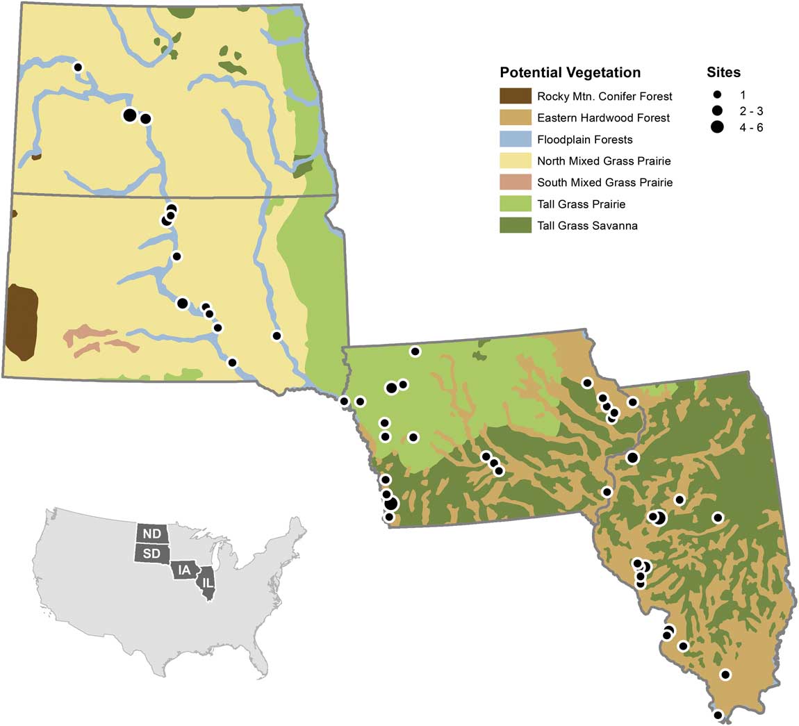
Figure 1 Location of sites used in analysis overlain on the Küchler vegetational zones (modified from Küchler [Reference Küchler1964] using data from Data Basin [U.S. Potential Natural Vegetation 2012]). Site localities are shown; circle sizes indicate presence of one or multiple sites in approximately the same location. Created by Brian Bills in ArcGIS, Version 10.2 (Environmental Systems Research Institute 2014) using data from Data Basin, CBI 2015, based on Küchler (Reference Küchler1964).
Most late Holocene faunal studies in North America are archaeological, with only four paleontological samples in this study. Three are in western Iowa: Thurman (970±150 RCYBP), Pleasant Ridge (1450±90 RCYBP), and Garrett Farm (3590±90 RCYBP), and one, Willard Cave (3500±60 to 1605±65 RCYBP), is in eastern Iowa (Semken and Falk Reference Semken and Falk1987). Each of these sites has its own inherent biases limiting the types and sizes of taxa incorporated. All other sites in the data set are archaeological. Naturally derived samples do occur within archaeological contexts (Sobolik Reference Sobolik1993), but various site types (cave, rock shelter, hunting camp, earth lodge, etc.) differentially filter assemblages (Croft and Semken Reference Croft and Semken1994; Semken and Graham Reference Semken and Graham1996).
Archaeologically, our sample represents diverse occupational histories. Nearly all Dakota-derived materials are from Late Prehistoric (ca. 1000 CE to 1650/1700 CE), Protohistoric (ca. 1650 CE/1700 to 1785 CE), and Historic (post-1785 CE) earth lodge villages (Semken and Falk Reference Semken and Falk1987). The western Iowa data are primarily derived from Late Prehistoric period cultural complexes: Glenwood, Great Oasis, and Oneota. The Garrett Farm paleontological site, also located in western Iowa, predates these cultural units and falls within the earlier Archaic time period. Sites in eastern Iowa include rock shelters, caves, and village occupations. All, except for Willard Cave, a paleontological sample, are associated with either Woodland (300 BCE to 900 CE) or Late Prehistoric (900 CE to 1500 CE) period cultural complexes.
Taphonomic pathways specific to archaeological sites include “cultural filters” like human coprolites, human selection of taxa and bones for differing cultural uses, attraction of scavenging animals to waste (Courtney and Fenton Reference Courtney and Fenton1976), entrapment in storage pits (Whyte Reference Whyte1991), and burials of humans and other animals (e.g., dogs), to name a few. Similarly, each site collection may contain taxa with substantially different body sizes (from shrews to bison) whose intrasite taphonomic pathways vary enormously both between and within sites sampled, or variation could be within site samples (Falk and Semken Reference Falk and Semken1998).
The faunal samples from each site were also subjected to significant postdepositional processes, including differing recovery techniques (Graham and Semken Reference Graham and Semken1987; Klippel et al. Reference Klippel, Snyder and Parmalee1987; Moreland Reference Moreland1994; Falk and Semken Reference Falk and Semken1998). These techniques, including screening with different mesh sizes, or lack thereof, are important taphonomic factors (Clark et al. Reference Clark, Beerbower and Kietzke1967; Shaffer and Sanchez Reference Shaffer and Sanchez1994; Semken and Graham, Reference Semken and Graham1996). Flotation techniques, another form of specimen recovery used for some samples, have their own biases, primarily the small amount of sediment processed for vertebrate faunal elements (Semken and Graham Reference Semken and Graham1996). Excavation procedures and tool selection (e.g., trowels, shovels, and the use of power equipment) also affect recovery and may alter the fauna recovered (Shaffer and Sanchez Reference Shaffer and Sanchez1994; Semken and Graham Reference Semken and Graham1996; Falk and Semken Reference Falk and Semken1998).
Methods
This data set consists of late Holocene (defined here as 4000–0 RCYBP) mammalian assemblages, derived from FAUNMAP (Faunmap Working Group Reference Graham and Lundelius1994) and the Neotoma Paleoecology Database (2010). In total, there are 73 site collections (samples) and 59 mammal taxa (variables) in the data set. Sites are both archaeological and paleontological in nature, with vertebrate taxa ranging in size from micromammals (insectivores and small rodents) to megamammals (bison). This data set is confined to those samples for which counts for minimum number of individuals (MNI) are presented (Grayson Reference Grayson1984). In order to extract a valid ecological signal from the data, domestic species, human remains, and taxa not identified to specific level were removed before ordinations were performed. Additionally, taxa occurring in only one site, usually represented by a single specimen, were removed.
Late Holocene faunal sites are not uniformly spaced with similar numbers of sites in specific geographic areas and a constant number of taxa per site. For these reasons, we have grouped our geographic samples by state political boundaries, realizing that they are independent of environmental boundaries, species ranges, and past cultural affiliations. It is easier to visualize states geographically rather than randomly selected, but unnamed, geographic areas of equal size. Also, state areas are frequently the domain of specific archaeologists and/or paleontologists, thus eliminating some biases introduced by multiple investigators, although this aspect can be highly variable. For example, one of the authors (H.A.S.) identified all of the micromammal material from the Iowa and Dakota sites, and another (C.R.F.) was involved in the excavation and/or analysis of most of the Dakota sites from which micromammals were recovered. Differences in taxonomic philosophy and excavation technique are thus minimized in the western end of the spectrum. Multiple individuals did the initial analyses and macrofaunal identifications from Illinois and Iowa.
Geographically, the sites are distributed across an east–west transect from Illinois through Iowa and into South and North Dakota. Today, this transect crosses the ecotone from hardwood forest in the east (Illinois) through the transition from forest (eastern Iowa) to tallgrass prairie (western Iowa) to tallgrass/shortgrass prairie (South and North Dakota). However, not all of the sites form an east–west transect sensu stricto within each state. With one exception noted earlier, the geographic distribution of the North and South Dakota sites is restricted to the Missouri River valley so they form a north–south trend through the two states, even though they are the western extent of the east–west transect. The Missouri River in the Dakotas broadly defines the ecotonal boundary between the tallgrass (east) and shortgrass (west) prairies (Fig 1.). In Iowa, the sites are widely distributed mostly along an east–west (moisture) transect. This transect spans the eastern hardwood, tall grass savanna, and tall grass prairie from the eastern third of the state to central and western Iowa, respectively. For Illinois, the sites range throughout the state and are generally arranged along a north–south temperature gradient. In addition, this transect captures both the deciduous forest and the Prairie Peninsula, an area of grassland intermixed with forest (Transeau Reference Transeau1935). Iowa also contains part of the Prairie Peninsula along its southern and eastern regions (Fig. 1). In essence, the configuration of the multistate transect is predominantly east–west but contains a southeastern–northwestern offset for the individual states. This orientation captures both moisture and temperature gradients, but these two variables are interrelated by effective moisture (precipitation minus evaporation), which limits the distributions of organisms. Hence, the gradient in this analysis is primarily one of moisture, as shown by the vegetation.
Recovery methods for faunal material vary greatly from site to site (Table 1). Excavated deposits can be entirely screened, selectively or partially screened, or not screened—depending on context, funding, research design, and the goals and interests of the investigator. Recovery design for samples that are selectively or entirely screened may involve use of a single screening technique or a combination of techniques, with variations in screen mesh size and volume of matrix processed using each technique. Table 2 shows the typical mesh size for the various screening techniques discussed in this study. Dry coarse screening involves processing excavated sediment through a coarse-mesh screen without the aid of any fluids. Fine-mesh screening nearly always involves water, using either naturally flowing or, more commonly, pressurized water to sieve (wash) sediments through a fine-mesh screen. Flotation is a general term for any method, mechanized or not, that uses water to separate the light fraction (materials that float) from the heavy fraction (materials that sink). In flotation, the heavy fraction that includes the vertebrate remains is generally retained by a mesh cloth or screen. If more than one recovery method was used at a single site (e.g., flotation and coarse screening), the method with the smallest mesh size and/or largest volume processed was counted for the purposes of analysis, and fine/water screening was assigned if even a portion of the material had been so processed. For example, if sediments are both water screened and floated, preference would be given to water screening. Finally, in cases in which more precise information about the screening method was not available, sites were simply identified as “screened” or “unscreened” where possible.
Table 1 Number of sites/state that used different recovery methods. FWS, fine/water screen; CS, coarse screen; CS/FL, coarse screen/flotation; FL, flotation; NS, not screened; NS/FL, not screened, but flotation. Screen mesh size for each method is given in Table 2.
Table 2 General mesh sizes used for screens used for faunal recovery techniques discussed.
Screening methods were obtained from faunal databases, site reports, or other publications (Hill Reference Hill1966; Kuttruff Reference Kuttruff1972; Van Dyke and Overstreet Reference Van Dyke and Overstreet1979; Styles Reference Styles1981; Tiffany Reference Tiffany1982; Emerson Reference Emerson1983; Milner Reference Milner1984; Colburn Reference Colburn1985; Wiant and Styles Reference Wiant and Styles1986; Cross Reference Cross1987; Semken and Falk, Reference Semken and Falk1987; Santure Reference Santure1990; Moffat et al. Reference Moffat, Koldehoff, Cremin, Martin, Masulis and McCorvie1992; Webb et al. Reference Webb, Anderson and Butler1992; McConaughy Reference McConaughy1993). Input from site excavators, including C.R.F., H.A.S., and R.W.G., was also incorporated. For the three sites from the Morton Mounds in Illinois (M13ILNW, M14ILNW, and M15ILNW), we did not find a specific reference to recovery methods other than use of shovels and smaller hand tools. Screens were apparently selectively used at Morton Mounds to recover small artifacts when necessary (Neumann Reference Neumann1937), but it is unclear whether they were used with animal bone. Because screening methods of any type were seldom used at this time for faunal recovery, we judge that sediments from that period were not screened.
We employed taxon lists from entire sites, rather than from individual portions of sites or strata. This was done for practical reasons; more detailed provenience data were not always available. That is, since we were interested in late Holocene assemblages, in those cases in which the sites had more than one late Holocene component, MNIs were summed. In many sites, the fauna were not broken down by component but were simply presented as summed site faunal lists. This approach places all sites on equal footing in terms of time-averaging processes like postdepositional burrowing (Erlandson Reference Erlandson1984; Bocek Reference Bocek1992) that can homogenize both site stratigraphy and faunal remains (see Grayson [Reference Grayson1984] and Lyman [Reference Lyman2008] for discussions of counting issues associated with aggregation). Species were categorized by their body size (Supplementary Table 2) based upon mass, accessed at Animal Diversity Web (2009). Size category 1 contains small mammals such as shrews and mice (<2 kg); size category 2 has medium-sized mammals (2–10 kg), including Procyon lotor and Marmota monax; and category 3 is large (>10 kg) mammals, including larger rodents (Castor canadensis) up to Bison bison.
All analyses were performed using R software (R Core Development Team 2011) and the ‘vegan’ package (Oksanen et al. Reference Oksanen, Blanchet, Kindt, Legendre, O’Hara, Simpson, Solymos, Henry, Stevens and Wagner2011). We used a square-root transformation followed by a Wisconsin double transformation to standardize our data set. Square-root transformation takes the square root of each value, behaving much like logarithmic transformation, assigning greater importance to rare species while compressing higher values—although the changes introduced through square-root transformation are less extreme than those from log transformation (McCune and Grace Reference McCune and Grace2002). Wisconsin standardization assigns a value to each species count in each sample, first relative to the species maximum, then to each sample total. We performed detrended correspondence analysis (DCA) of the state data sets as well as of the full four-state data set. This method allows researchers to compare multivariate data sets by reducing these data sets to a limited number of independent axes reflecting sources of variation in the data set. Using the same procedure, we also performed non-metric multidimensional scaling (NMDS) analyses and compared the results with those of the DCA analysis. The analyses revealed the same general patterns, and we have included comparative plots in the Supplementary Data (Supplementary Figs. 1–3).
Results
Analysis of these smaller-scale state data sets and the larger composite four-state data set indicates differences in outcomes based on the relative strengths of the environmental gradient versus the recovery method employed. If the ordinations depicted the environmental gradient, then they should show clusters of species with adaptations for moister conditions to the east and southeast and those adapted to much drier environments in the west and northwest. Specifically, forested environments and species (Sciurus spp., Tamias striatus, Scalopus aquaticus, etc.) are found in the east–southeast with taxa (Bison bison, Antilocapra americana, Perognathus flavescens, Chaetodipus hispidus, etc.) adapted to drier grassland environments occurring in the Dakotas to the west–northwest. Because it is in the steepest segment of the prairie/forest ecotone, Iowa would have an intermixture of forest and grassland.
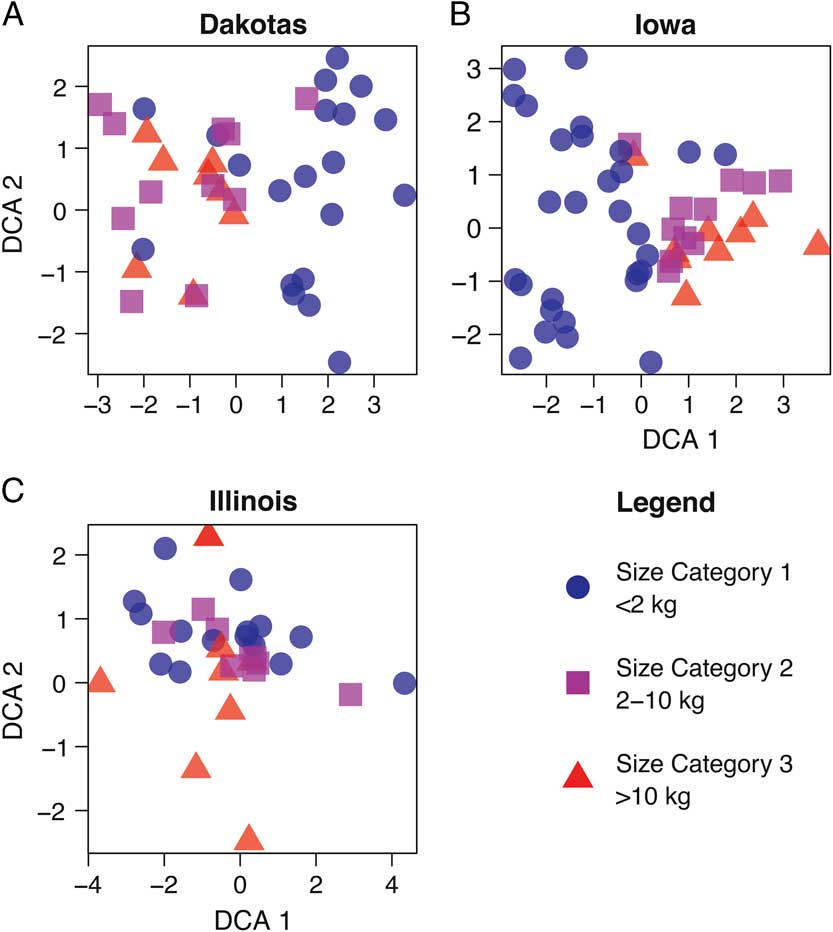
Figure 2 depicts DCA plots showing the relationships between sites and species for the area considered (NMDS plots for the same data are provided in Supplementary Figures 1–3). Instead of clusters identifying environmental adaptations, as would be expected for an environmental gradient, the clusters reflect the body size of the animals (Supplementary Table 2). It is important to note that some sites contained mammals from all size categories. From these plots, it is apparent that the body size of the mammals, not environmental factors, is driving the species ordinations at the state level (Fig. 2).

Figure 2 DCA biplot of North and South Dakota (A), Iowa (B), and Illinois (C) assemblages, based on taxon size.
To explore this taphonomic effect further, we then examined the method of recovery for each site (Fig. 3, Supplementary Table 1). When comparing the similarity in patterns for Figures 2 and 3, it is clear that body size corresponds strongly with method of collection, especially screen mesh size. Those sites not fine screened or water screened tend to group together (Fig. 3), in accordance with the larger taxa they contain (Fig. 2). The screen mesh size used has created an artificial sorting of sites according to the body size of animals recovered. Specifically (Fig. 2A,B), small mammals of size category 1 form their own unique cluster, whereas medium (size category 2) and large (size category 3) groups cluster together. In some cases, the small mammal–dominated sites will cluster with the medium and large mammal–dominated ones. The clusters for DCA attributes (Fig. 3) and NMDS parameters (Supplementary Fig. 2) differ slightly in presentation, but the clusters identified by each method share a similar interpretation.
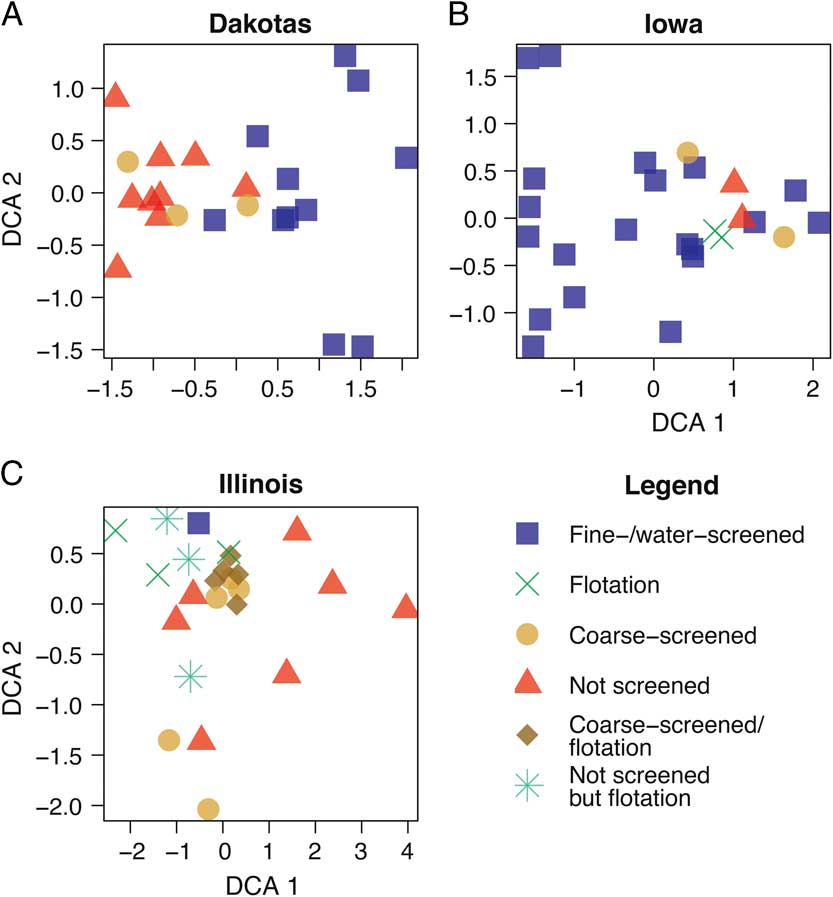
Figure 3 DCA biplot of North and South Dakota (A), Iowa (B), and Illinois (C) sites by recovery method.
The ordination pattern for Illinois (Fig. 3C) is quite different in comparison to the ordinations for Iowa and the Dakotas. In Figure 3C, most of the coarse-screened sites form a tight cluster, along with one flotation site. If the size of the cluster is enlarged to cover the NW corner of the plot, then it contains the only fine-/water-screened site in the sample as well as four additional flotation sites and two unscreened sites. As a whole, unscreened sites are broadly distributed across the DCA1 axis, whereas the flotation sites range along the DCA2 axis.
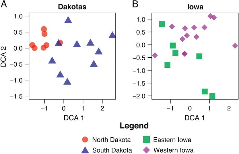
Next, to assess the effects of collecting techniques on the potential environmental signal, only the animals that clustered within the fine-/water-screening method were ordinated for North and South Dakota and Iowa (Fig. 4), and only archaeologically derived sites are included. Illinois was not included, because there is only one fine-/water-screened site. Body size and collection techniques should not be a factor in the ordinations of these samples. For North and South Dakota, Bagnell and Fort George were removed, because they lacked size category 1 mammals; Anton Rygh, Medicine Crow, Jiggs Thompson, and Kipp’s Post each had fewer than five small individuals total and were also removed. The North and South Dakota samples (Fig. 4A) show a clear differentiation of sites by species composition (i.e., habitat types). This plot (Fig. 4A) suggests the environmental gradient (temperature) between North and South Dakota is more clearly captured when only small mammals are considered. The North Dakota sites contain species adapted to cooler and moister habitats (e.g., Myodes [= Clethrionomys] gapperi, Microtus pennsylvanicus, Sorex cinereus), as would be expected; whereas the South Dakota sites contain species more adapted to drier habitats (Dipodomys ordii, Chaetodipus hispidus, Peroganthus flavus, etc.).

Figure 4 DCA biplot restricted to size category 1 (<2 kg) for North and South Dakota (A) and eastern and western Iowa (B) sites by geographic location.
For Iowa (Fig. 4B), in order to have as many samples as possible, Clarkson and Kingston are retained despite small sample sizes of small mammals. Garrett Farm, Pleasant Ridge, Thurman, and Willard Cave (noncultural) are removed. The present environmental gradient is the strongest in Iowa, where the pattern for the micromammal component and environmental inference is not as clear but present. Most western Iowa sites appear to form a relatively cohesive cluster with three outliers centered on the middle of DCA2. Two of these outliers group with the eastern Iowa cluster (Fig. 4B). In this analysis, there is a significant difference in the DCA (Fig. 4B) and the NMDS (Supplementary Fig. 3B) presentations, in that the intermingling of eastern and western area sites is greater in NMDS. In other words, DCA is better at separating the clusters.
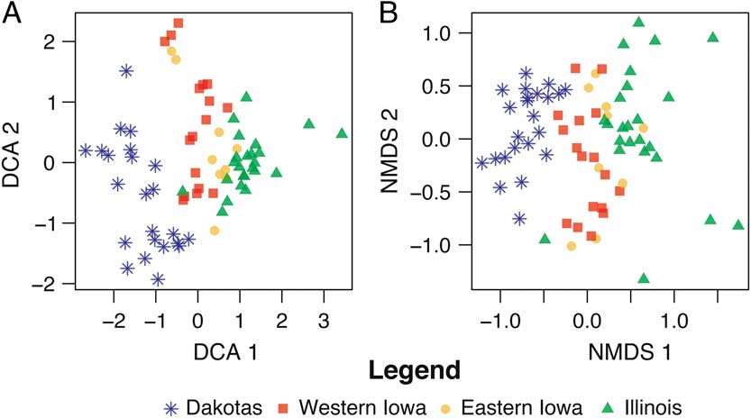
In Figure 5, we view both the DCA (5A) and NMDS (5B) ordination results of the entire data set, combining all four states. The full data set, it will be recalled, contains sites transecting a substantial environmental gradient, spanning from the plains in the west to the eastern deciduous hardwood forest. This larger data set is simply an unfiltered compilation (taphonomic factors have not been removed) of the state data sets discussed earlier. Yet these ordinations show a dramatically stronger pattern than those performed for the individual states. Here, we see a clear gradient from west to east, with sites plotting in proximity to others from the same environment. As with the smaller state data sets discussed earlier, diverse body sizes and different collecting techniques are present within this sample, but they do not seem to alter the multistate environmental signal as they did for the individual states. In comparing Figure 5A and B, again it appears that DCA does a better job of separating the clusters, especially those of eastern and western Iowa.

Figure 5 Comparison of DCA (A) and NMDS (B) biplots of full data set, with all sites across four states, and all taxa from all three size categories included.
Discussion
We have used both DCA and NMDS to examine the effects of taphonomy on the analysis of environmental gradients. Both NMDS and DCA are indirect ordination techniques. One primary difference between the two techniques is that NMDS does not make any underlying assumptions about the structure of the data. DCA reformats the data by detrending (a brute force method for flattening the horseshoe arch created by correspondence analysis) and rescaling them before it conducts any analyses (see Patzkowsky and Holland [Reference Patzkowsky and Holland2012] for detailed discussion of techniques).
A variety of papers argue for or against the use of either DCA or NMDS, with many critical of DCA because of data transformation (e.g., Faith et al. Reference Faith, Minchin and Belbin1987; Minchin Reference Minchin1987; Whittaker Reference Whittaker1987; Cao et al. Reference Cao, Bark and Williams1997; Ramete Reference Ramete2007; Patzkowsky and Holland Reference Patzkowsky and Holland2012). To test the validity of these methods in analyzing gradients, Patzkowsky and Holland (Reference Patzkowsky and Holland2012) conducted two types of statistical analyses on synthetically constructed gradients. First, they compared DCA and NMDS methods by examining the Spearman’s rank correlation for each method. The results showed that both DCA and NMDS are good at calculating axis 1, but DCA is more effective for reconstructing axis 2. They then examined the two methods by calculating the root-mean-square error of a Procrustes fit (Patzkowsky and Holland Reference Patzkowsky and Holland2012). In this comparison, they found that DCA outperformed NMDS when axis 1 becomes relatively longer than axis 2 (Patzkowsky and Holland Reference Patzkowsky and Holland2012), which is the case in our samples. For these two reasons, we have used DCA in our presentation, but we also report NMDS plots in Supplementary Figures 1–3. We did not detect substantial differences between DCA and NMDS in any of the analyses, except in placement of various sites that are the result of the methods used by each technique. The clusters defined by both DCA and NMDS were not substantially different (compare DCA plots in the text [Figs. 1–4] with NMDS plots in Supplementary Figs. 1–3). For the most part, it appears that DCA and NMDS were equally effective at defining clusters of sites and species in these analyses. In this study, DCA tended to separate clusters better than NMDS, as discussed earlier, although the interpretations of the clusters produced by either DCA or NMDS would be similar.
Multivariate analyses of state-by-state subsets yield little insight into environmental gradients when sites with the full range of taxon sizes are included. Instead, ordinations within state areas are driven by taphonomic processes. Most importantly, recovery methods including flotation, fine/water screening, coarse screening, and shovel/trowel excavation without screening varied significantly. These methodological differences not only profoundly affected the number of total individuals in a sample, but also created a substantial body-size bias, with larger species disproportionately represented in samples that were not finely screened and smaller taxa more concentrated in fine- or water-screened assemblages. Because hundreds of kilograms to tons of sediment may be processed by water screening, this process yields the majority of microfaunal specimens at sites. The abundances of such taxa are often strongly correlated with the local environment (Stahl Reference Stahl1982; Semken and Falk Reference Semken and Falk1987, Reference Semken and Falk1991). Their absence may muddle or weaken the environmental signal. We may expect to lose entirely the signal these taxa provide at sites that are coarse screened, or not screened at all, where visibility of large bones determines whether faunal specimens are recovered to be included in subsequent analysis.
Figure 3 clearly illustrates this point. The tightest cluster (centered at axis 1=0.0 and axis 2=0.3) of the Illinois sites (Fig. 3C) is primarily defined by coarse-screened sites with one flotation site and one fine-/water-screened site. As noted previously, the other flotation sites, unscreened sites, and coarse-screened sites are broadly distributed without forming any clusters. In other words, based on the identified species in the plot, recovery techniques and corresponding body sizes of taxa in each collection appear to be intermixed, unlike the plots for Iowa (Fig. 3B) and the Dakotas (Fig. 3A), where there are distinctions. This phenomenon is probably due to the similarities of the three collection techniques—coarse screened, not screened, and flotation—that generally do not collect diverse small mammal remains. Flotation, which generally uses only liters of sediment, is excellent for recovering plant macrofossils (Struever Reference Struever1968), but because of the small size of the sediment sample, it may not be an effective means of recovering diverse small mammal remains. On the other hand, flotation may be very effective for aquatic resources (fish, snails, etc.) (Styles Reference Styles1981). The association of the only fine-/water-screened site with coarse-screened sites may be the result of the volume of material screened as well, which is not known. If only a small volume of sediment was processed by fine/water screening, then this process would be similar to flotation. We suggest that flotation methods should be supplemented by fine/water screening for greatest recovery of small mammals.
We further attempted to uncover the environmental signal within states by removing large taxa, thereby negating the size-related taphonomic bias and leaving the more environmentally sensitive micromammals (Stahl Reference Stahl1982; Semken and Falk Reference Semken and Falk1987). With large taxa removed, the Illinois data set yielded a sample too small for analysis, as noted earlier in the discussion of screening methods. The eastern Iowa sites intergrade with the western Iowa sites (Fig. 4B), with the steeper ecotone between grassland to the west and deciduous forest to the east. In analysis of the North and South Dakota data set, only micromammal taxa (Fig. 4) reveal a clear environmental signal with an environmental gradient from the moister and cooler northern sites to the more arid southern sites. This latitudinal gradient reflects decreasing mean annual temperature to the north (Mitchel Reference Mitchel1976), resulting in greater effective moisture. Conversely, warmer temperatures to the south reduce effective moisture, creating more arid conditions.
Additionally exacerbating the damped environmental signal was the limited degree of the environmental gradient sampled by each state (Fig. 1). Even in Iowa, where the environmental gradient (prairie–forest ecotone) is now most pronounced climatically and vegetationally, the strongest signal proved to be screening method (compare Figs. 2B and 3B). Larger animals grouped together and apart from smaller taxa, as previously observed by Semken and Graham (Reference Semken and Graham1996). Part of this modulation may result from the fact that, at the state scale, the environmental gradient is not strong enough to separate faunas. The DCA (Fig. 4B) of the eastern and western Iowa faunas seems to separate the biotas of these two regions; the NMDS (Supplementary Fig. 2) does not reflect any differentiation. Furthermore, even one taxon, if sufficiently dominant in some assemblages (and absent in others), may also strongly influence where each site lands on the plot. For example, strongly bison-dominated localities tend to be in western states, while bison counts taper off to the east and other taxa, more woodland-adapted (e.g., Odocoileus virginianus, Ursus americanus), dominate. This pattern is consistent with the small mammal pattern of species adapted to drier habitats (Cynomys ludovicianus, Perognathus flavus, Dipodomys ordii) occurring farther to the west, and those of moister habitats (Tamias striatus, Sciurus sp., Blarina sp., Marmota monax) to the east.
Larger-scale analysis of the full data set reflects the overall environmental gradient, from full prairie in the west to deciduous forest in the east (Figs. 1 and 5), even though taphonomic factors have not been removed in this data set. The gradient here is substantially stronger than it is at the scale of either two states or individual states, although the DCA of the Iowa sites shows some differentiation of eastern and western faunas. With rare exceptions, environments grade into one another, forming ecotones; thus, some overlap of corresponding sites (reflecting the overlap of underlying environment) is not only acceptable but is to be expected.
There may be several reasons for the dominance of the paleoenvironmental signal when the entire gradient is considered. First, the environmental gradient in smaller areas (i.e., states) may be relatively weak in comparison to the overall gradient, except for the case in South and North Dakota (Fig. 4A). In other words, species turnover within a state is significantly less than along the entire gradient; consequently, taphonomy drives the ordination. The size of the geographic area and strength of the environmental gradient, therefore, are fundamental factors in determining whether ordinations of samples primarily will be driven by taphonomy or environment. Part of this may also relate simply to sample size of sites, which can be a function of geographic area. The number of sites in each state is significantly smaller than the total number of sites across the environmental gradient, even though the geographic areas of individual states vary. Furthermore, sites in one area may be geographically concentrated along a prominent feature (e.g., Dakota sites along the Missouri River) and others broadly dispersed throughout the state (e.g., Iowa). Increasing the number of sites also increases the number of taphonomic pathways, which may result in swamping any individual taphonomic signal. At any rate, the most critical aspect of the geographic sample is that it spans the geographic extent of the environmental gradient.
Taphonomic versus environmental signals compete for dominance in these ordination analyses. At the smaller state scale, the environmental gradients are weak, except for the north–south gradient in the Dakotas. Taphonomy provides the stronger signal at smaller scales, but across the vast span of the entire data set and the environmental gradient, the environmental signal overrides taphonomy. These results also suggest that if an environmental gradient is exceptionally strong in a small area, a single state or smaller unit (e.g., an alpine transect), the environmental pattern may emerge in the ordinations, even though the taphonomic biases have not been eliminated, although the prairie–forest ecotone in Iowa did not override taphonomy. Also, these results assume that the sample sizes of sites and fauna are large enough.
Conclusions
Multivariate analyses of initial state-by-state subsets transecting the prairie–forest ecotone in North America yielded little insight into geographical or environmental gradients between sites. Rather, taphonomic factors and, in particular, differences in recovery method (Fig. 3) provide the overriding signal. DCA and NMDS analyses revealed the underlying environmental gradient when applied to the entire geographic area (Fig. 5). This study highlights the impact of collection methodology on subsequent paleoecological analyses, particularly when the goal is to understand paleoecological patterns in specific or limited geographic areas. Taphonomic and site recovery factors may mask the environmental signals that are of interest to paleontologists and archaeologists. Hence, workers attempting paleoenvironmental comparisons must consider collection technique as a paramount factor in recovering environmental data from comparison of multisite assemblages. These analyses document that fine/water screening is the best method of recovery for mammal remains for paleoecological analysis. In fact, we recommend that fine/water screening supplement flotation for the best recovery of micromammals.
Both DCA and NMDS analyses are a useful means of distinguishing environmental differences among sites derived from strong gradients over larger geographic areas. DCA appears to better separate clusters than does NMDS but the overall patterns are basically the same. In other words, taphonomic signals appear to be scale dependent, similar to the species/area effect (MacArthur and Wilson Reference MacArthur and Wilson1967) in biodiversity. Consequently, with sufficient geographic area and/or strong environmental gradients, the environmental signal will shine through. Although our work was restricted to late Holocene mammalian assemblages, it has broader applications to paleoecological studies in which different methodologies might result in sample fractionation.
Acknowledgments
We thank M. Patzkowsky (Pennsylvania State University [PSU]) for instruction and helpful suggestions regarding the DCA and NMDS analyses. He, R. Alley (PSU), E. Post (PSU), and R. W. Graham (PSU) served on L.E.M.’s dissertation committee, and she wishes to thank them for their support and suggestions for improving the manuscript. B. Bills (PSU) is gratefully acknowledged for his assistance in the creation of Figure 1. Thank you to Beckie Dyer (Illinois State Museum) for providing citation information. Steven L. DeVore (National Park Service) and David Gradwohl (Iowa State University) are thanked for providing information about collection techniques used at the Cribb’s Crib site, as is Walter Klippel (University of Tennessee) for his help in gathering collection information for the Morton Mound sites. Screening data for the Noble-Weiting site were taken from an unpublished master’s thesis by Arlene Rose Schilt (1977) at the Department of Anthropology and Sociology, Illinois State University, Normal. Sue Anne Graham is thanked for proofreading the final manuscript. National Science Foundation (NSF) grant EAR0948652 supported L.E.M. NSF grants EAR0948652 and EAR 0622349 supported the Neotoma Paleoecology Database. We also thank two anonymous reviewers and the editor for their insightful suggestions, but we are responsible for any errors or misinterpretations.
Supplementary material
Data available from the Dryad Digital Repository: https://doi.org/10.5061/dryad.s6fd5c6