


1. Introduction
Model-based approaches rooted in linear systems theory have helped shed light on the nature of energy amplification mechanisms in flows of interest. It has been shown through linear analyses, for instance, that the transient energy growth in channel flows is due to the non-normality of the linearized Navier–Stokes operator governing the dynamics of perturbations about the well-known laminar parabolic velocity profile (Schmid & Henningson Reference Schmid and Henningson2001). Jovanović & Bamieh (Reference Jovanović and Bamieh2005) and McKeon & Sharma (Reference McKeon and Sharma2010), on the other hand, have investigated energy amplification mechanisms in channel flows and turbulent pipe flow by studying the linearized response to perturbations, via input–output analysis or resolvent analysis. Likewise, Symon et al. (Reference Symon, Rosenberg, Dawson and McKeon2018) have recently investigated the resonance and pseudoresonance mechanisms in low-Reynolds-number cylinder flow and turbulent pipe flow using similar techniques. Although these analyses provide valuable insight into the amplification mechanisms of given flows, they do so under the assumption of small amplitude fluctuations about a steady base flow (often the temporal mean). Furthermore, because of the time-invariant nature of the chosen base flow, such methods are inherently incapable of capturing the cross-frequency interactions that are responsible for the energy transfer between motions at different time scales. Not only are these cross-frequency interactions the fundamental mechanisms behind the energy cascade in turbulent flows, but they are also responsible for the rise of complex dynamics in laminar flows such as boundary layers (Mittal, Kotapati & Cattafesta Reference Mittal, Kotapati and Cattafesta2005) and mixing layers (Ho & Huang Reference Ho and Huang1981). The limitations of these analyses are of course known and have partly been addressed in the past. For instance, Jovanović & Fardad (Reference Jovanović and Fardad2008) introduced a perturbation analysis framework to study the amplification mechanisms of linear, small-amplitude, time-periodic systems and applied it to two-dimensional oscillating channel flow. More recently, Rigas, Sipp & Colonius (Reference Rigas, Sipp and Colonius2020), analysed the transition to turbulence in a boundary layer by seeking the flow structure that would maximize the shear stress at the wall through the nonlinear Navier–Stokes operator in the frequency domain. Shaabani-Ardali, Sipp and Lesshafft (Reference Shaabani-Ardali, Sipp and Lesshafft2020), on the other hand, implemented a time-domain analysis to compute the time-periodic inlet forcing that would maximize mixing about a time-periodic base flow in a bifurcating jet. We extend the resolvent framework in order to address the limitations of linear time-invariant analyses, while still providing insight into the input–output characteristics of the fluid flow at hand.
We note that the energy production, dissipation and transfer in fluid flows have also been studied using techniques other than the aforementioned input–output framework. Majda & Timofeyev (Reference Majda and Timofeyev2000), for instance, analysed the statistical dynamics and energy transfer mechanisms in the inviscid Burgers equation by performing a harmonic balance in wavenumber space. Noack et al. (Reference Noack, Schlegel, Ahlborn, Mutschke, Morzyński, Comte and Tadmor2008), on the other hand, leveraged Galerkin projection techniques to reduce the dimensionality of the Reynolds-averaged Navier–Stokes equation and develop a reduced-order model for the flow of energy in cylinder flow and homogeneous shear turbulence.
This paper considers a framework we call harmonic resolvent analysis, in which the dynamics are expanded about a periodically time-varying base flow, which can be viewed as the large-scale coherent structures of the flow. It will be shown in § 2 that this formulation justifies treating the higher-order terms in the expansion as small input disturbances. Analysing the linearized governing equations in the frequency domain enables the explicit computation of the harmonic resolvent, a linear operator which governs the dynamics of small perturbations about the time-varying, periodic base flow. Because of the multimodal nature of the base flow, the harmonic resolvent can capture the leading-order cross-frequency interactions, which arise in the form of triadic couplings between perturbations at frequencies  $\omega$ and
  $\alpha$ through the base flow at frequency
  $\omega -\alpha$. The number of triads that can be captured is determined by the number of Fourier modes that are retained in the base flow and we show that if the latter is simply a steady flow, then resolvent analysis is recovered. The harmonic resolvent operator can be viewed as a special case of the harmonic transfer function introduced by Wereley (Reference Wereley1991), which maps inputs to outputs in the space of exponentially modulated periodic signals. Furthermore, it is worth mentioning that the temporal expansion of the dynamics about the large-scale coherent structures of the flow that we perform is similar to the wavenumber-space expansions applied in the generalized quasilinear approximation introduced by Marston, Chini & Tobias (Reference Marston, Chini and Tobias2016) to describe the interaction between the large and small scale of flows in the context of direct statistical simulations.
Similarly to the spectral analysis of the resolvent operator, the singular value decomposition of the harmonic resolvent provides insight into the amplification mechanisms of disturbances about the time-varying base flow. Specifically, the right and left singular vectors of the operator are the optimal spatio-temporal forcing and the most amplified spatio-temporal response patterns, respectively. It will be shown that one can also seek the optimal spatial forcing and most amplified spatial response at selected frequency pairs in order to study their cross-frequency amplification mechanisms.
In § 3 we illustrate the method on a system of three ordinary differential equations, whose low dimensionality and time-periodic dynamics allow us to illustrate the characteristics of the harmonic resolvent and to draw a natural comparison between the harmonic resolvent framework and the usual resolvent analysis.
Finally, in § 4 we consider the flow over an airfoil at near-stall angle of attack. This flow exhibits multichromatic time-periodic dynamics, which we study using the harmonic resolvent. In particular, we compute the optimal forcing and response modes via the singular value decomposition of the harmonic resolvent, and we analyse the amplification mechanisms of perturbations about the periodically time-varying base flow that arises from the nonlinear dynamics.
2. Mathematical formulation
In this section, we define the harmonic resolvent operator, first for a general nonlinear system and then for incompressible fluid flows.
2.1. General nonlinear system
We consider the nonlinear autonomous system
 \begin{equation} \frac{\textrm{d}}{\textrm{d}t}{\boldsymbol{q}}(t) = {\boldsymbol{f}}\left({\boldsymbol{q}}(t)\right) \end{equation}
with state  ${\boldsymbol {q}}(t)$. In three-dimensional incompressible fluid flows, the state is the three-dimensional vector velocity field along with the scalar pressure.
In the harmonic resolvent framework, we are interested in studying the amplification mechanisms of small perturbations  ${\boldsymbol {q}}'(t)$ about a time-varying base flow that is periodic with period
  $T$, given by
 \begin{equation} {\boldsymbol{Q}}(t) = \sum_{\omega \in \Omega_b} \hat{\boldsymbol{Q}}_{\omega}\,\textrm{e}^{\textrm{i}\,\omega t}, \end{equation}
with  $\Omega _b\subset ({2{\rm \pi} }/{T})\mathbb {Z}$. The base flow does not need to satisfy the governing equations and
  $\Omega _b$ usually contains a small subset of frequencies that approximate the dynamics of the large coherent structures present in the flow. We proceed by seeking perturbations of the form
 \begin{equation} {\boldsymbol{q}}'(t) = \sum_{\omega \in \Omega}\hat{\boldsymbol{q}}'_{\omega}\,\textrm{e}^{\textrm{i}\,\omega t}, \end{equation}
with  $\Omega \subset ({2{\rm \pi} }/{T})\mathbb {Z}$. Usually
  $\Omega _b \subset \Omega$, as
  $\Omega$ is the set of temporal frequencies associated with the flow structures that one wishes to resolve. (In general, the set
  $\Omega$ need not be restricted to multiples of the fundamental frequency
  $2{\rm \pi} /T$, although we do make this assumption in this paper.) Upon substituting the decomposition
  ${\boldsymbol {q}}(t)={\boldsymbol {Q}}(t)+{\boldsymbol {q}}'(t)$ in (2.1) we obtain
 \begin{equation} \frac{\textrm{d}}{\textrm{d}t}{\boldsymbol{q}}'(t) = \underbrace{\mathcal{D}_{{\boldsymbol{q}}}{\,\boldsymbol{f}}\left({\boldsymbol{Q}}(t)\right)}_{{\boldsymbol{\mathsf{A}}}(t)}{\boldsymbol{q}}'(t) + {\boldsymbol{h}}'(t), \end{equation}
where
 \begin{equation} {\boldsymbol{h}}'(t) = \left[-\frac{\textrm{d}}{\textrm{d}t}{\boldsymbol{Q}}(t) + {\boldsymbol{f}}\left({\boldsymbol{Q}}(t)\right)\right] + o\left(\|{\boldsymbol{q}}'(t)\|\right). \end{equation}
The first term in (2.5) is the error associated with the base flow not satisfying the governing equations, while the second represents the higher-order terms in the dynamics. Before proceeding further, we observe that  ${\boldsymbol{\mathsf{A}}}(t)$ is periodic with period
  $T$ (since
  ${\boldsymbol {Q}}$ is periodic), and it can therefore be represented in terms of a Fourier series, analogous to (2.2). We then obtain the following expression for the perturbation at frequency
  $\omega$:
 \begin{equation} \textrm{i}\,\omega \hat{\boldsymbol{q}}'_{\omega} = \sum_{\alpha\in \Omega} \hat{\boldsymbol{\mathsf{A}}}_{\omega-\alpha} \hat{\boldsymbol{q}}'_{\alpha} + \hat{\boldsymbol{h}}'_{\omega} \quad \forall \omega \in \Omega. \end{equation}
We neglect frequencies  $\omega$ that are not in
  $\Omega$. For ease of notation, let
  $\hat {\boldsymbol {q}}'$ be the vector of
  $\hat {\boldsymbol {q}}'_\omega$ for all frequencies
  $\omega \in \Omega$, and let
  $\hat {\boldsymbol {h}}'$ be defined similarly. We then define the operator
  ${\boldsymbol{\mathsf{T}}}$ by
 \begin{equation} \big[{\boldsymbol{\mathsf{T}}}\hat {\boldsymbol{q}}'\big]_\omega = \textrm{i}\,\omega \hat {\boldsymbol{q}}_\omega' - \sum_{\alpha\in\Omega} \hat {\boldsymbol{\mathsf{A}}}_{\omega-\alpha}\hat {\boldsymbol{q}}_\alpha'. \end{equation}
 Before introducing the formal definition of the harmonic resolvent, it is necessary to address a subtlety. If the base flow  ${\boldsymbol {Q}}(t)$ is an exact solution of (2.1), then
  ${\boldsymbol{\mathsf{T}}}$ is singular and its null space contains a vector associated with the neutrally stable direction of phase shift about the base flow given by the Fourier coefficients of
  $({\textrm {d}}/{\textrm {d}t}) {\boldsymbol {Q}}(t)$. Similarly, if
  ${\boldsymbol {Q}}(t)$ is an approximate solution of (2.1), then
  ${\boldsymbol{\mathsf{T}}}$ is nearly singular along the direction of phase shift. In either case, effects associated with shifting the original base flow in time can dominate and obscure the genuine amplification mechanisms of interest. We define the harmonic resolvent in a way that removes the phase shift and preserves the desired steady-state periodic response up to a constant shift in time. In particular, we restrict
  ${\boldsymbol{\mathsf{T}}}$ to a subspace
  $\Sigma$ that is orthogonal to the direction of phase shift given by
  $\widehat{\textrm{d}{\boldsymbol{Q}}/{\textrm{d}t}} $. This is analogous to constructing a Poincaré map by reducing the dynamics onto a codimension-1 surface pierced by the limit cycle (Guckenheimer & Holmes Reference Guckenheimer and Holmes2002). We notice that when we take
  $\hat {\boldsymbol {q}}'\in \Sigma$, (2.6) ensures that
  ${\boldsymbol {h}}'$ must be in the range of the restricted operator
  ${\boldsymbol{\mathsf{T}}} \vert _{\Sigma }$. Therefore, we define the harmonic resolvent operator on
  $W_{\Sigma } = Range ({\boldsymbol{\mathsf{T}}} \vert _{\Sigma } )$ as
 \begin{equation} {\boldsymbol{\mathsf{H}}} = \left( \left. {\boldsymbol{\mathsf{T}}} \right\vert_{\Sigma} \right)^{{-}1}. \end{equation}
Details on efficient computation with this operator can be found in appendix A.
Finally, after removing the phase shift, (2.6) may be written as
 \begin{equation} \hat{\boldsymbol{q}}' = {\boldsymbol{\mathsf{H}}}\hat{\boldsymbol{h}}', \end{equation}
where  $\hat {\boldsymbol {q}}'\in \Sigma$, and
  ${\boldsymbol {h}}'\in W_{\Sigma }$ now live in compatible codimension-1 subspaces. Therefore, the harmonic resolvent describes the steady-state dynamics of small periodic perturbations
  $\hat {\boldsymbol {q}}'$ about a periodic base flow in response to a periodic input forcing
  $\hat {\boldsymbol {h}}'$, up to a constant shift in time. Note that, if external inputs are present (such as a control input, or noise forcing the system), these enter into the formulation in the same way that
  ${\boldsymbol {h}}'$ does, and this leads to the harmonic transfer function of Wereley (Reference Wereley1991). A more thorough discussion of the characteristics of the harmonic resolvent and its connection with the usual resolvent operator is given at the end of § 2.2.
2.2. Bilinear system: incompressible fluid flow
We now consider an incompressible fluid flow governed by the Navier–Stokes equations, given by
 \begin{equation} \begin{array}{c} \dfrac{\partial}{\partial t}{\boldsymbol{u}} + {\boldsymbol{u}}\boldsymbol{\cdot} \boldsymbol{\nabla} {\boldsymbol{u}} ={-}\boldsymbol{\nabla} p + Re^{{-}1}\nabla^2 {\boldsymbol{u}} ,\\ \boldsymbol{\nabla} \boldsymbol{\cdot} {\boldsymbol{u}} = 0. \end{array} \end{equation}
Here,  ${\boldsymbol {u}}({\boldsymbol {x}},t)$ and
  $p({\boldsymbol {x}},t)$ are the velocity and pressure, respectively, over the spatial domain
  $\mathcal {X}\subseteq \mathbb {R}^3$. For ease of notation, we will drop the explicit dependence on
  ${\boldsymbol {x}}$ from here on. Equation (2.10) can be written compactly as
 \begin{equation} \frac{\partial}{\partial t} \underbrace{\begin{bmatrix} {\boldsymbol{\mathsf{I}}} & 0 \\ 0 & 0 \end{bmatrix}}_{{\boldsymbol{\mathsf{M}}}} \begin{bmatrix} {\boldsymbol{u}}(t)\\ p(t)\end{bmatrix} = \underbrace{\begin{bmatrix} Re^{{-}1}\nabla^2 & -\boldsymbol{\nabla} \\ -\boldsymbol{\nabla} \boldsymbol{\cdot} & 0 \end{bmatrix}}_{{\boldsymbol{\mathsf{L}}}} \begin{bmatrix}{\boldsymbol{u}}(t)\\ p(t)\end{bmatrix} + \underbrace{\begin{bmatrix} -{\boldsymbol{u}}(t)\boldsymbol{\cdot} \boldsymbol{\nabla} {\boldsymbol{u}}(t) \\ 0 \end{bmatrix}}_{{\boldsymbol{g}}\left({\boldsymbol{u}}(t),{\boldsymbol{u}}(t)\right)}. \end{equation}
We denote the state vector by  ${\boldsymbol {q}}=({\boldsymbol {u}},p)$, and consider perturbations about a periodic base flow, as in § 2.1,
 \begin{equation} {\boldsymbol{q}}(t) = {\boldsymbol{Q}}(t)+{\boldsymbol{q}}'(t) = \sum_{\omega \in \Omega_b}\hat{\boldsymbol{Q}}_{\omega}\,\textrm{e}^{\textrm{i}\,\omega t} + \sum_{\omega \in \Omega}\hat{\boldsymbol{q}}'_{\omega}\,\textrm{e}^{\textrm{i}\,\omega t}, \end{equation}
where  $\Omega _b \subseteq \Omega \subset ({2{\rm \pi} }/{T})\mathbb {Z}$. As before, we seek an input–output representation for the perturbations
  ${\boldsymbol {q}}'$. Substituting (2.12) in (2.11), and neglecting frequencies
  $\omega \notin \Omega$, we obtain
 \begin{equation} \textrm{i}\,\omega {\boldsymbol{\mathsf{M}}} \hat{\boldsymbol{q}}'_{\omega} = {\boldsymbol{\mathsf{L}}} \hat{\boldsymbol{q}}'_{\omega} + \sum_{\alpha \in \Omega}\big[{\boldsymbol{g}}(\hat{\boldsymbol{Q}}_{\omega-\alpha},\hat{\boldsymbol{q}}'_{\alpha}) + {\boldsymbol{g}}(\hat{\boldsymbol{q}}'_{\alpha},\hat{\boldsymbol{Q}}_{\omega-\alpha})\big] + \hat{\boldsymbol{h}}'_{\omega},\quad \forall \omega \in \Omega , \end{equation}
where, as in the previous section,  $\hat {\boldsymbol {h}}'_{\omega }$ is the Fourier mode of the base flow error along with the terms that are nonlinear in
  $\hat {\boldsymbol {q}}'_\omega$ (see (2.5)). We again let
  $\hat {\boldsymbol {q}}'$ denote the vector of
  $\hat {\boldsymbol {q}}_\omega '$ for all frequencies
  $\omega \in \Omega$, and define the operator
  ${\boldsymbol{\mathsf{T}}}$ by
 \begin{equation} \big[{\boldsymbol{\mathsf{T}}}\hat{\boldsymbol{q}}'\big]_\omega = (\textrm{i}\,\omega {\boldsymbol{\mathsf{M}}} - {\boldsymbol{\mathsf{L}}})\hat{\boldsymbol{q}}'_\omega -\sum_{\alpha\in\Omega} \big[{\boldsymbol{g}}(\hat{\boldsymbol{Q}}_{\omega-\alpha},\hat{\boldsymbol{q}}'_{\alpha}) + {\boldsymbol{g}}(\hat{\boldsymbol{q}}'_{\alpha},\hat{\boldsymbol{Q}}_{\omega-\alpha}) \big]. \end{equation}
Finally, after removing the phase shift, as per the discussion at the end of § 2.1, (2.13) may be written compactly as
 \begin{equation} \hat{\boldsymbol{q}}' = {\boldsymbol{\mathsf{H}}}\hat{\boldsymbol{h}}'. \end{equation}
Also, as specified at the end of § 2.1, inputs such as a control signal or an external disturbance enter in the system in the same way as  ${\boldsymbol {h}}'$.
At this point, a few comments on the structure of the harmonic resolvent operator are in order. First, note that the number of frequencies in the set  $\Omega$ may be infinite (e.g.
  $\Omega =({2{\rm \pi} }/{T})\mathbb {Z}$), in which case the harmonic resolvent is an infinite-dimensional operator. However, in practice, one truncates its dimensionality by selecting a finite number of frequencies
  $\omega \in \Omega$ that are considered to be of interest. The dimension of
  ${\boldsymbol{\mathsf{H}}}$ is therefore proportional to the number of frequencies in
  $\Omega$. As mentioned previously, we usually consider the frequencies
  $\Omega _b$ in the base flow to be a subset of the frequencies
  $\Omega$ of the perturbations. That is, one usually wishes to study the dynamics of perturbations at multiple frequencies, about a filtered representation of the large-scale structures that are observed in the flow. The number of frequencies
  $\omega \in \Omega _b$ affects the accuracy of the linear operator in representing the nonlinear dynamics of the flow. This becomes clear once we observe from (2.13) that perturbations at different temporal frequencies are linearly coupled to one another via the base flow. More precisely, structures at frequency
  $\omega$ are coupled to structures at frequency
  $\alpha$ through the base flow at the frequency difference
  $\omega - \alpha$. Of course,
  $\omega -\alpha$ needs to be in
  $\Omega _b$ if one wishes to capture the aforementioned interaction. For instance, if the base flow has frequencies
  $\Omega _b = \{-\omega,0,\omega \}$ and we want to study the dynamics of perturbations over the set of frequencies
  $\Omega = \{-2\omega,-\omega,0,\omega,2\omega \}$, then
 \[ {\boldsymbol{\mathsf{T}}} = \begin{bmatrix} {\boldsymbol{\mathsf{R}}}^{{-}1}_{{-}2\omega} & {\boldsymbol{\mathsf{G}}}_{-\omega} & 0 & 0 & 0\\ {\boldsymbol{\mathsf{G}}}_\omega & {\boldsymbol{\mathsf{R}}}^{{-}1}_{-\omega} & {\boldsymbol{\mathsf{G}}}_{-\omega} & 0 & 0\\ 0 & {\boldsymbol{\mathsf{G}}}_\omega & {\boldsymbol{\mathsf{R}}}^{{-}1}_{0} & {\boldsymbol{\mathsf{G}}}_{-\omega} & 0\\ 0 & 0 & {\boldsymbol{\mathsf{G}}}_\omega & {\boldsymbol{\mathsf{R}}}^{{-}1}_\omega & {\boldsymbol{\mathsf{G}}}_{-\omega}\\ 0 & 0 & 0 & {\boldsymbol{\mathsf{G}}}_\omega & {\boldsymbol{\mathsf{R}}}^{{-}1}_{2\omega}\\ \end{bmatrix}, \]
where
 \begin{gather*} {\boldsymbol{\mathsf{G}}}_\omega {\boldsymbol{q}} ={-}{\boldsymbol{g}}(\hat{\boldsymbol{Q}}_\omega,{\boldsymbol{q}}) - {\boldsymbol{g}}({\boldsymbol{q}},\hat{\boldsymbol{Q}}_\omega),\\ {\boldsymbol{\mathsf{R}}}^{{-}1}_\omega = \textrm{i}\,\omega {\boldsymbol{\mathsf{M}}} - {\boldsymbol{\mathsf{L}}} + {\boldsymbol{\mathsf{G}}}_0. \end{gather*}
Note that  ${\boldsymbol{\mathsf{R}}}_\omega$ is the usual resolvent operator at frequency
  $\omega$ (i.e. the resolvent of the operator linearized about the constant base flow
  $\hat {\boldsymbol {Q}}_0$). In fact, in the special case that the base flow is constant (i.e.
  $\Omega _b=\{0\}$), the harmonic resolvent becomes block diagonal, and perturbations at different frequencies are decoupled.
Finally, we wish to make a remark about the resolvent formalism. Whether the base flow is time varying or time invariant, (2.13) is exactly equivalent to the Navier–Stokes equations if  $\hat {{\boldsymbol {h}}}'_{\omega }$ is known. This introduces a convenient splitting of the dynamics into linear and nonlinear parts, where the linear part is amenable to classical input–output analyses; this is the point of view taken by McKeon & Sharma (Reference McKeon and Sharma2010), for instance. If
  $\hat {{\boldsymbol {h}}}'_{\omega }$ is unknown, but can be modelled as random noise (as in McKeon & Sharma (Reference McKeon and Sharma2010)), the linear part evaluated about the temporal mean provides useful insight into the dominant amplification mechanisms. If, on the other hand,
  $\hat {{\boldsymbol {h}}}'$ has some structure (e.g. large-scale coherent structures at some dominant frequency), then the linearization about the temporal mean may not be useful, if the deviations are large. In the harmonic resolvent framework, we extend the input–output analysis of the linearized Navier–Stokes operator to flows that exhibit such large periodic deviations from the mean.
2.3. Global amplification mechanisms from the harmonic resolvent
The mathematical formulation presented in the previous sections leads to a linear time-periodic input–output system in Fourier space, represented by
 \begin{equation} \hat{\boldsymbol{q}}' = {\boldsymbol{\mathsf{H}}}\hat{\boldsymbol{w}}', \end{equation}
where the harmonic resolvent  ${\boldsymbol{\mathsf{H}}}$ governs the dynamics of perturbations about a periodic base flow
  $\hat {\boldsymbol {Q}}$ in response to some periodic forcing
  $\hat {\boldsymbol {w}}'$. There are several ways to view the perturbation
  $\hat {\boldsymbol {w}}'$. From the point of view of control theory,
  $\hat {\boldsymbol {w}}'$ can be interpreted as an external input, which might be chosen to achieve some control objective. In a more physics-driven approach,
  $\hat {\boldsymbol {w}}'$ can be understood as the frequency-domain representation of the nonlinearities that feed back into the linear harmonic resolvent. Alternatively,
  $\hat {\boldsymbol {w}}'$ can be viewed as an external disturbance that perturbs the system around a known periodic orbit.
In any of these circumstances, one may want to understand the dominant mechanisms by which space–time inputs are amplified through  ${\boldsymbol{\mathsf{H}}}$. One way to do so is by seeking a unit-norm space–time input
  $\hat {\boldsymbol {w}}'$ that leads to the most amplified space–time response
  $\hat {\boldsymbol {q}}'$. Formally,
 \begin{equation} \begin{array}{c} \displaystyle\max_{\hat{\boldsymbol{w}}'} \quad \langle{\boldsymbol{\mathsf{H}}}\hat{\boldsymbol{w}}', {\boldsymbol{\mathsf{H}}}\hat{\boldsymbol{w}}'\rangle \\ \text{subject to } \quad \langle \hat{\boldsymbol{w}}',\hat{\boldsymbol{w}}'\rangle = 1. \\ \end{array} \end{equation}
It can be shown that (2.17) leads to the eigenvalue problem
 \begin{equation} {\boldsymbol{\mathsf{H}}}^{*}{\boldsymbol{\mathsf{H}}}\hat{\boldsymbol{\psi}} = \sigma \hat{\boldsymbol{\psi}}, \end{equation}
where the optimal unit-norm forcing  $\hat {\boldsymbol {\psi }}$ is the first right singular vector of
  ${\boldsymbol{\mathsf{H}}}$, and
  $\sigma$ is the largest singular value. If we left-multiply (2.18) by
  ${\boldsymbol{\mathsf{H}}}$ and define
  $\hat {\boldsymbol {\phi }} = {\boldsymbol{\mathsf{H}}}\hat {\boldsymbol {\psi }}$ we obtain
 \begin{equation} {\boldsymbol{\mathsf{H}}}{\boldsymbol{\mathsf{H}}}^*\hat{\boldsymbol{\phi}} = \sigma \hat{\boldsymbol{\phi}} , \end{equation}
from which we can conclude that the optimal (most amplified) response,  $\hat {\boldsymbol {\phi }}$, is the corresponding left singular vector of
  ${\boldsymbol{\mathsf{H}}}$. We will refer to the right singular vectors of
  ${\boldsymbol{\mathsf{H}}}$ as input modes and we will refer to the left singular vectors as output modes.
Proceeding further, the response of the linear time-periodic system to an arbitrary input  $\hat {\boldsymbol {w}}'$ can be expressed as a linear combination of input and output modes of the harmonic resolvent, as follows:
 \begin{equation} \hat{\boldsymbol{q}}' = {\boldsymbol{\mathsf{H}}}\hat{\boldsymbol{w}}'=\sum_{j = 1}^{N-1}\sigma_j\hat{\boldsymbol{\phi}}_j\underbrace{\hat{\boldsymbol{\psi}}_j^*\hat{\boldsymbol{w}}'}_{\langle\hat{\boldsymbol{w}}', \hat{\boldsymbol{\psi}}_j \rangle}, \end{equation}
where  $\hat {{\boldsymbol {\phi }}}_j, \hat {{\boldsymbol {\psi }}}_j \in \mathbb {C}^N$. Observe that we sum to
  $N-1$ since, as per the discussion at the end of § 2.1, we have constrained the range of
  ${\boldsymbol{\mathsf{H}}}$ to an
  $(N-1)$-dimensional subspace orthogonal to
  $\widehat{\textrm{d}{\boldsymbol{Q}}/{\textrm{d}t}}$. Equation (2.20) sheds some light on the information contained within the output and input modes. In particular, the output modes
  $\hat {\boldsymbol {\phi }}_j$ form an orthonormal basis for the range of
  ${\boldsymbol{\mathsf{H}}}$ and identify the spatio-temporal structures that are preferentially excited in response to some external input. The input modes
  $\hat {\boldsymbol {\psi }}_j$ form an orthonormal basis for the domain of
  ${\boldsymbol{\mathsf{H}}}$ and identify the spatio-temporal structures that are most effective at exciting an energetic response. That is, the input modes relate to the spatio-temporal sensitivity of the flow to external inputs. This concept can be easily understood in terms of the inner product in the underbrace of (2.20). As an example, let us consider a rank-1 approximation of
  ${\boldsymbol{\mathsf{H}}}$ and assume that
  $\sigma _1 \approx 1$. If the external input
  $\hat {\boldsymbol {w}}'$ aligns poorly with the input mode
  $\hat {\boldsymbol {\psi }}_1$, then
  $\langle \hat {\boldsymbol {w}}', \hat {\boldsymbol {\psi }}_1 \rangle \ll 1$ and consequently
  $\|\hat {\boldsymbol {q}}'\|\ll 1$, meaning that
  $\hat {\boldsymbol {w}}'$ is not effective at exciting a very energetic response through the harmonic resolvent. On the other hand, if the external input aligns well with
  $\hat {\boldsymbol {\psi }}_1$, then
  $\langle \hat {\boldsymbol {w}}', \hat {\boldsymbol {\psi }}_1 \rangle \approx \|\hat {\boldsymbol {w}}'\|$. Consequently
  $\hat {\boldsymbol {q}}' \approx \hat {\boldsymbol {\phi }}_1 \|\hat {\boldsymbol {w}}'\|$ and
  $\|\hat {\boldsymbol {q}}'\|\approx \|\hat {\boldsymbol {w}}'\|$. In this case
  $\hat {\boldsymbol {w}}'$ is (close to) optimal and it excites the (close to) optimal most energetic response. Understanding the sensitivity information contained within the input modes is especially important if one is interested in controlling the flow. For instance, if
  $\hat {\boldsymbol {w}}'$ is a chosen control input, it is advisable to design it in such a way that
  $\langle \hat {\boldsymbol {w}}',\hat {\boldsymbol {\psi }}_j\rangle$ is maximized.
The singular values  $\sigma _j$ can be understood as the gains on the input–output pairs
  $\hat {\boldsymbol {\psi }}_j$,
  $\hat {\boldsymbol {\phi }}_j$ and they provide information about the rank of the harmonic resolvent. For instance, if
  $\sigma _j$ is very small, then the corresponding modes have little effect on the input–output response and can be neglected. Often the effective rank
  $r$ of
  ${\boldsymbol{\mathsf{H}}}$ (i.e. the number of singular values that exceed some threshold) is such that
  $r \ll N-1$, and
  ${\boldsymbol{\mathsf{H}}}$ may be approximated as
 \begin{equation} {\boldsymbol{\mathsf{H}}} \approx\sum_{j = 1}^{r}\sigma_j\hat{\boldsymbol{\phi}}_j\hat{\boldsymbol{\psi}}_j^*. \end{equation}
We would like to add that the low rank property of the harmonic resolvent could likely be exploited to develop reduced-order models for the nonlinear dynamics of the flow about the periodic orbit under consideration. For instance the dimension of the nonlinear algebraic system (2.6) in the frequency domain could be reduced by projecting onto the leading input and output modes of the harmonic resolvent. However, investigating this idea further is beyond the scope of the present work.
2.4. Cross-frequency amplification mechanisms from the harmonic resolvent
The global analysis that was carried out in the previous section can be easily extended to selected frequency pairs or selected subsets of  $\Omega$. Since the harmonic resolvent accounts for the coupling between different frequencies, we may ask which cross-frequency interactions are most significant. More precisely, for given
  $\alpha ,\omega \in \Omega$, we can seek the unit-norm forcing at frequency
  $\alpha$ that triggers the most amplified response at frequency
  $\omega$. This corresponds to the following optimization problem:
 \begin{equation} \begin{array}{c} \displaystyle \max_{\hat{\boldsymbol{w}}'_{\alpha}} \quad \langle \hat{\boldsymbol{q}}'_{\omega},\hat{\boldsymbol{q}}'_{\omega} \rangle \\ \text{subject to } \quad \langle \hat{\boldsymbol{w}}'_{\alpha},\hat{\boldsymbol{w}}'_{\alpha} \rangle = 1, \end{array} \end{equation}
where
 \begin{equation} \hat{\boldsymbol{q}}'_{\omega} = {\boldsymbol{\mathsf{H}}}_{\omega,\alpha}\hat{\boldsymbol{w}}'_{\alpha}, \end{equation}
and where  ${\boldsymbol{\mathsf{H}}}_{\omega ,\alpha }$ is the block of
  ${\boldsymbol{\mathsf{H}}}$ that couples structures at frequency
  $\omega$ with structures at frequency
  $\alpha$. It can be shown that the optimal input
  $\hat {\boldsymbol {w}}'_{\alpha }$ and the optimal output
  $\hat {\boldsymbol {q}}'_{\alpha }$ are, respectively, the first right singular vector and the first left singular vector of
  ${\boldsymbol{\mathsf{H}}}_{\omega ,\alpha }$. The corresponding singular value,
  $\sigma _{\omega ,\alpha }$, is the gain on the
  $\omega ,\alpha$ cross-frequency pair. For different values of
  $\omega ,\alpha \in \Omega$, the magnitudes of
  $\sigma _{\omega ,\alpha }$ provide a measure to determine which cross-frequency couplings are responsible for the development of the structures that are observed in the full nonlinear flow.
3. Application to a three-dimensional toy model
The objective of this section is to illustrate, through a simple model, the benefits of using the harmonic resolvent framework to analyse fluid flows that exhibit features that arise from nonlinear mechanisms. The signature of such flows is a non-monochromatic energy spectrum, which highlights the action of the nonlinear term in distributing energy across selected frequencies. We consider a three-dimensional system of ordinary differential equations defined as follows:
 \begin{equation} \left.\begin{array}{c} \dot x = {\mu} x - {\gamma} y - {\alpha} x z - {\beta} x y, \\ \dot y = {\gamma} x + {\mu} y - {\alpha} y z + {\beta} x^2, \\ \dot z ={-}{\alpha} z + {\alpha} \left(x^2 + y^2 \right), \end{array}\right\} \end{equation}
where  $\dot x$ denotes
  $\textrm {d}x/\textrm {d}t$, and
  $\alpha ,\gamma ,\mu >0$. A simple rescaling of time allows us to take
  $\gamma =1$ without loss of generality, so henceforth we assume
  $\gamma =1$.
Although we do not claim that this toy model represents any specific fluid flow, it does share some features with the Navier–Stokes equations. Like the Navier–Stokes equations, the nonlinearities are quadratic and energy conserving. Recall that a dynamical system  $\textrm{d}\boldsymbol{q}/\textrm{d}t = {\boldsymbol {f}}({\boldsymbol {q}})$ is energy conserving if
 \begin{equation} \frac{\textrm{d}}{\textrm{d}t} \frac{1}{2}\|{\boldsymbol{q}}\|^2 = \langle \, {\boldsymbol{f}}\left({\boldsymbol{q}} \right),{\boldsymbol{q}} \rangle = 0. \end{equation}
For the Navier–Stokes equations, with typical boundary conditions on  ${\boldsymbol {u}}$ (e.g.
  ${\boldsymbol {u}}={\boldsymbol {0}}$ on the boundary, or
  ${\boldsymbol {u}}$ tangent to the boundary), one finds
  $\langle {\boldsymbol {u}}\boldsymbol {\cdot } \boldsymbol {\nabla } {\boldsymbol {u}},{\boldsymbol {u}} \rangle = 0$, so the nonlinear terms in (2.10) are energy conserving. Similarly, for our toy model, the nonlinear terms
  ${\boldsymbol {f}}(x,y,z)=(-\alpha xz-\beta xy,-\alpha yz+\beta x^2,\alpha (x^2+y^2))$ satisfy
  ${\boldsymbol {f}}({\boldsymbol {q}})\boldsymbol {\cdot }{\boldsymbol {q}}=0$, and hence are energy conserving. In addition, we remark that the system (3.1) is closely related to the reduced-order model of the flow past a cylinder used by Noack et al. (Reference Noack, Afanasiev, Morzynski, Tadmor and Thiele2003), and the well-known Stuart–Landau model (Stuart Reference Stuart1958).
It is useful to transform the model (3.1) to polar coordinates; with  $x=r\cos \theta$ and
  $y=r\sin \theta$, the dynamics become
 \begin{gather} \dot r = (\mu-\alpha z)r, \end{gather}
 \begin{gather}\dot \theta = 1 + \beta r\cos\theta, \end{gather}
 \begin{gather}\dot z = \alpha(r^2-z). \end{gather}
In these coordinates, it is clear that if  $\beta ^2<\alpha /\mu$, there is a limit cycle at
  $r^2=z=\mu /\alpha$. Furthermore, by integrating (3.3b), we find that the period of the limit cycle is
  $T =2{\rm \pi} /\sqrt {1-\beta ^2\mu /\alpha }$, so the fundamental frequency of the limit cycle is
 \begin{equation} \omega=\sqrt{1-\beta^2\mu/\alpha}. \end{equation}
We proceed by briefly analysing how the dynamics of the system change as one varies the parameter  $\beta$.
When  $\beta = 0$, the dynamics in the
  $\theta$ direction become
  $\dot \theta =1$, so the system is rotationally symmetric about the
  $z$-axis. Moreover, the limit cycle is monochromatic, with frequency
  $\omega =1$. Figure 1 shows the limit cycle and its energy spectrum, for
  $\mu =\alpha =1/5$ and
  $\beta =0$.

Figure 1. Results for the toy problem (3.1) with  $\beta =0$ and
  $\mu =\alpha =1/5$, showing (a) energy spectrum on the limit cycle and (b) (projected) limit cycle colour coded according to the angular speed
  $\dot {\theta }$ (3.3b). The marker located at
  $(x,y) = (0,0)$ in panel (b) indicates the temporal mean of the limit cycle.
Next, we consider the dynamics for  $0<\beta <\sqrt {\alpha /\mu }$. There is still a limit cycle at
  $r^2=z=\mu /\alpha$, but now we see from (3.3b) that there is an asymmetry: when
  $x>0$, the angular speed
  $\dot \theta$ increases, and when
  $x<0$, the angular speed decreases. This will cause the state to spend more time on the left half of the limit cycle, and so the temporal mean is shifted to the left, as shown in figure 2(b). In addition, multiple harmonics are introduced into the frequency spectrum, as shown in figure 2(a). Note also that the fundamental frequency of the limit cycle is now slightly less than 1 (
 $\omega = 0.9798$), according to (3.4).

Figure 2. Analogue of figure 1 for  $\beta =1/5$, showing (a) energy spectrum and (b) (projected) limit cycle. Higher harmonics are present in the energy spectrum. Furthermore, the angular speed varies around the limit cycle according to (3.3b) and the temporal mean is consequently shifted away from 0.
Before proceeding, we remark that frequency prediction, global stability analysis and the geometric decay of Fourier modes in flows that exhibit time-periodic limit cycles have been the subject of extensive studies. Dušek, Gal & Fraunié (Reference Dušek, Gal and Fraunié1994), for instance, developed a theoretical framework to explain the observed hierarchy of harmonics in the spectrum of the wake of a circular cylinder. More recently, Sipp & Lebedev (Reference Sipp and Lebedev2007) studied the linearized Navier–Stokes operators about base and mean flows in the cylinder wake and in an open cavity. Finally, Turton, Tuckerman & Barkley (Reference Turton, Tuckerman and Barkley2015) presented results regarding the prediction of the limit cycle frequency in thermosolutal convection.
3.1. Comparison between the harmonic resolvent framework and resolvent analysis
In this section we compare the effectiveness of different linearizations in predicting the response of the nonlinear system to some external periodic forcing. For this purpose, we introduce forcing to (3.1) with parameters  $\mu = \alpha =\beta = 1/5$
 \begin{equation} \left.\begin{array}{c} \dot x = \mu x - y - \alpha x z - \beta x y + w_1' ,\\ \dot y = x + \mu y - \alpha y z + \beta x^2 + w_2' ,\\ \dot z ={-}\alpha z + \alpha \left(x^2 + y^2 \right) \end{array}\right\} \end{equation}
and define  ${\boldsymbol {w}}'(t)=(\varepsilon \sin (\omega t), \varepsilon \cos (\omega t))$ as our external periodic forcing at the fundamental frequency
  $\omega = 0.9798$ (from (3.4)) and with
  $\varepsilon = 0.1$. The forcing
  ${\boldsymbol {w}}'(t)$ can be expanded in a Fourier series
 \begin{equation} {\boldsymbol{w}}'(t) = \sum_{k \in \{{-}1,1\}} \hat{\boldsymbol{w}}'_{k}{\rm e}^{\textrm{i}\, k\omega t}, \end{equation}
and the dynamics of perturbations  ${\boldsymbol {q}}'(t)$ about a given base flow in response to
  ${\boldsymbol {w}}'(t)$ can be written as
 \begin{equation} \hat{\boldsymbol{q}}' = {\boldsymbol{\mathsf{H}}}{\boldsymbol{\mathsf{B}}}\hat{\boldsymbol{w}}', \end{equation}
where  ${\boldsymbol{\mathsf{H}}}$ is the harmonic resolvent evaluated about the chosen base flow and
  ${\boldsymbol{\mathsf{B}}}$ is a block-diagonal operator through which the input
  $\hat {\boldsymbol {w}}'$ enters the system. Throughout this section we consider perturbations with spectral energy content up to the seventh harmonic of the fundamental frequency
 \begin{equation} {\boldsymbol{q}}'(t) = \sum_{k ={-}7}^{7}\hat{\boldsymbol{q}}_{k}{\rm e}^{\textrm{i}\,k\omega t}, \quad \Omega = \{{-}7\omega,-6\omega, \ldots ,7\omega \}, \end{equation}
and we compare the predictions obtained by linearizing about the temporal mean  $\Omega _b = \{0\}$ (see the marker in figure 2b) to predictions obtained by linearizing about the exact limit cycle
  $\Omega _b = \{-3\omega ,\ldots ,3\omega \}$ (see figure 2a). (Recall that linearizing about the mean is equivalent to performing resolvent analysis.) The results are compared against a ground truth computed by numerical integration of (3.5). In recalling from § 2.1 that the range of the harmonic resolvent is orthogonal to any phase shift about the chosen base flow, we warn the reader that in order to draw a direct comparison between the harmonic resolvent results and the nonlinear simulation, it may be necessary to phase match the forced solution
  ${\boldsymbol {q}}(t)$ from (3.5) to the base flow
  ${\boldsymbol {Q}}(t)$. Specifically, we advance (3.5) for a few forcing periods until transients have decayed, and then we phase match in the least squares sense
 \begin{equation} \min_{\phi \in \mathbb{R}} \quad \sum_{\omega \in \Omega_b} \big\vert \big\vert \hat{{\boldsymbol{q}}}_{\omega}\,\textrm{e}^{\textrm{i}\,\omega \phi } - \hat{{\boldsymbol{Q}}}_{\omega}\big\vert \big\vert_2^2. \end{equation}
Finally, the aforementioned ground truth perturbation is given by  ${\boldsymbol {q}}'(t) = {\boldsymbol {q}}(t) - {\boldsymbol {Q}}(t)$.
Figure 3 shows the energy spectrum of the post-transient perturbations  $\hat {\boldsymbol {q}}'$ in response to the periodic input
  $\hat {\boldsymbol {w}}'$ as well as the state evolution
  ${\boldsymbol {q}}'(t)$ over one fundamental period. We observe from the nonlinear simulation that forcing at frequency
  $\omega$ leads to a response with energy content also at the zeroth, second and third harmonics. We observe also that the prediction obtained by linearizing about the exact limit cycle accurately matches the ground truth. This is because the time-varying base flow about which we evaluate the harmonic resolvent couples structures at different frequencies and we are therefore able to predict (to first order) the frequency off-scatter that is observed in the nonlinear system. The extent to which we are able to capture cross-frequency interactions is given by the block singular values of
  ${\boldsymbol{\mathsf{H}}}$ shown in figure 4(b). We colour code the cross-frequency blocks according to the fractional variance
 \begin{equation} E_{j,k} = \frac{\displaystyle\sum_{m = 1}^3 \sigma^2_{m,\left(\,j,k\right)}}{\displaystyle\sum_{n = 1}^{N-1}\sigma_n^2}, \end{equation}
where  $\sigma _{m,(\,j,k)}$ is the
  $m$th singular value of the
  $(\,j\omega ,k\omega )$ block of
  ${\boldsymbol{\mathsf{H}}}$ and
  $\sigma _n$ is the
  $n$th singular value of
  ${\boldsymbol{\mathsf{H}}}$. The normalization is such that
  $\sum _{j,k} E_{j,k} = 1$. We observe from the
  $1\omega$-column in figure 4(b) that forcing at the fundamental frequency may trigger a response with spectral energy content up to the third harmonic, and that is precisely what the energy spectrum in figure 3(a) confirms.

Figure 3. Response of the system (3.5) to periodic forcing at the fundamental frequency  $\omega = 0.9798$. (a) Normalized spectrum of the perturbation
  $\boldsymbol {q'}(t)$ and (b) state evolution over one period
  $T = 2{\rm \pi} /\omega$. Symbols:
  $\ast$, Ground truth computed by numerical integration of (3.5);
  $\square$, harmonic resolvent prediction with
  $\Omega _b = \{-3\omega ,\ldots ,3\omega \}$;
  $\diamond$, harmonic resolvent prediction with
  $\Omega _b = \{0\}$ (equivalent to resolvent analysis).


Linearizing about the temporal mean, however, does not provide an accurate representation of the response of the nonlinear system to the given periodic forcing at frequency  $\omega$. First, observe that through this linearization we overestimate the spectral energy at the fundamental frequency. Second, it is clear from figures 3(a) and 3(b) that the prediction is monochromatic at frequency
  $\omega$. This is because
  ${\boldsymbol{\mathsf{H}}}$ is block diagonal, as mentioned at the end of § 2.2 and illustrated in figure 4(a). Therefore, no cross-frequency interaction can be accounted for through the base flow, and forcing at frequency
  $\omega$ will only produce a response at the same frequency.
4. Application to flow past an airfoil at near-stall angle of attack
We now consider two-dimensional incompressible flow past an airfoil at an angle of attack, under conditions for which there is unsteady vortex shedding. We perform numerical simulations using the immersed boundary formulation of Taira & Colonius (Reference Taira and Colonius2007), to compute the flow past a NACA 0012 airfoil at angle of attack of  $20^\circ$ and Reynolds number of
  $200$ based on the chord. The immersed boundary formulation enforces no-slip boundary conditions at the surface
  $\mathcal {S}$ of the airfoil by imposing a body force
  ${\boldsymbol {f}}$, as expressed below
 \begin{equation} \left.\begin{array}{c} \displaystyle \frac{\partial}{\partial t}{\boldsymbol{u}} + {\boldsymbol{u}}\boldsymbol{\cdot} \boldsymbol{\nabla} {\boldsymbol{u}} ={-}\boldsymbol{\nabla} p + Re^{{-}1} \nabla^2 {\boldsymbol{u}} + \int_{\mathcal{S}}{\boldsymbol{f}}({\boldsymbol{\xi}})\delta({\boldsymbol{\xi}} - {\boldsymbol{x}})\,\textrm{d}{\boldsymbol{\xi}},\\ \boldsymbol{\nabla} \boldsymbol{\cdot} {\boldsymbol{u}} = 0, \\ \displaystyle{\boldsymbol{u}}({\boldsymbol{\xi}}) = \int_{\mathcal{X}}{\boldsymbol{u}}({\boldsymbol{x}})\delta({\boldsymbol{x}} - {\boldsymbol{\xi}})\,\textrm{d}{\boldsymbol{x}} = 0,\quad\text{for } {\boldsymbol{\xi}}\in\mathcal{S}, \end{array}\right\} \end{equation}
where  ${\boldsymbol {u}}({\boldsymbol {x}},t)$ and
  $p({\boldsymbol {x}},t)$ are the velocity and pressure over the spatial domain
  $\mathcal {X} = \mathbb {R}^2$, and
  $\delta$ is the Dirac delta function. The third equation in (4.1) is a set of algebraic constraints that enforce the no-slip boundary condition on the surface
  $\mathcal {S}$. We refer the reader to Taira & Colonius (Reference Taira and Colonius2007) for a detailed discussion of the method.
We centre the half-chord of the airfoil at the origin of the computational domain of size  $[-4,12]\times [-2.5,2.5]$ and we discretize the domain on a
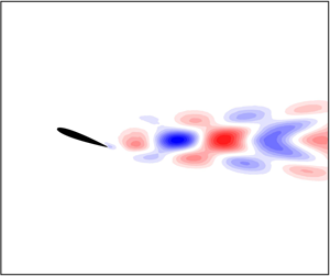
  $800\times 250$ grid. We impose a uniform inflow boundary condition at the inlet, slip-wall boundary conditions at the top and bottom boundaries and a convective outflow boundary condition at the outlet. The vorticity spectrum is shown in figure 5(a), while a representative snapshot of the mean-subtracted vorticity field on the limit cycle is shown in figure 5(b). We observe that up to five harmonics of the fundamental frequency
  $\omega = 2.40$ are active on the limit cycle, suggesting that non-trivial nonlinear mechanisms are at play.

Figure 5. Nonlinear simulation of flow past an airfoil, showing (a) global vorticity spectrum and (b) snapshot of vorticity fluctuation on the limit cycle.
In the upcoming analysis we take our state vector to be  ${\boldsymbol {q}}=({\boldsymbol {u}},p,{\boldsymbol {f}})$ and we expand the dynamics about a chosen base flow
  ${\boldsymbol {Q}}(t)$. We omit the spatial dependence of the states for notational simplicity. Moreover, we consider perturbations
  ${\boldsymbol {q}}'(t)$ over the set of frequencies
  $\Omega = \{-7\omega ,\ldots ,7\omega \}$. Upon linearizing the dynamics about the chosen base flow we obtain the linear input–output system
 \begin{equation} \hat{\boldsymbol{q}}' = {\boldsymbol{\mathsf{H}}}\hat{\boldsymbol{w}}' = \sum_{j = 1}^{N-1} \sigma_j\hat{\boldsymbol{\phi}}_{j}\hat{\boldsymbol{\psi}}^*_{j}\hat{\boldsymbol{w}}' , \end{equation}
where  $\hat {\boldsymbol {w}}'$ is the frequency-domain representation of the nonlinear terms that feed back into the linear harmonic resolvent. The left singular vector
  $\hat {\boldsymbol {\phi }}_j$ is the
  $j$th global output mode and the right singular vector
  $\hat {\boldsymbol {\psi }}_j$ is the
  $j$th global input mode. We wish to specify that
  ${\boldsymbol{\mathsf{H}}}$ is not computed explicitly since it is a dense operator of prohibitive size
  $N \sim O(10^7)$. Specifically, given the
  $n$-dimensional state vector
  ${\boldsymbol {q}}'$ and
  $15$ frequencies in
  $\Omega$, the size of the harmonic resolvent is
  $N = 15n$. Instead, given
  ${\boldsymbol{\mathsf{T}}}$, which is a sparse operator whose non-zero entries depend on the spatial discretization scheme used on the governing equations, we computed the leading singular values and singular vectors of
  ${\boldsymbol{\mathsf{H}}}$ using one of the randomized singular value decomposition algorithms in Halko, Martinsson & Tropp (Reference Halko, Martinsson and Tropp2011). The implementation was carried out with an in-house solver based on the PETSc (Balay et al. Reference Balay, Abhyankar, Adams, Brown, Brune, Buschelman, Dalcin, Dener, Eijkhout and Gropp2019) and SLEPc (Hernandez, Roman & Vidal Reference Hernandez, Roman and Vidal2005) libraries. Additional details on the implementation can be found in appendix A.
4.1. Amplification mechanisms about a time-varying base flow
We linearize the dynamics in (4.1) about a time-periodic base flow over the set of frequencies  $\Omega _b =\{-3\omega ,\ldots ,3\omega \}$ with
  $\omega = 2.40$ as in figure 5(a), and we compute the singular value decomposition of the harmonic resolvent.
First, note from figure 6(a) that there is more than an order of magnitude separation between the first and the second singular values of the harmonic resolvent and we can therefore argue that the harmonic resolvent has low-rank structure.

Figure 6. Singular values of the harmonic resolvent for flow past an airfoil with  $\Omega _b = \{-3\omega ,\ldots ,3\omega \}$,
  $\Omega = \{-7\omega ,\ldots ,7\omega \}$ and
  $\omega = 2.40$, showing (a) singular values of
  ${\boldsymbol{\mathsf{H}}}$ and (b) blockwise fractional variance
  $E_{j,k}$ defined by an expression similar to (3.10).
Second, figure 6(b) shows that the nonlinear flow is very susceptible to perturbations at the fundamental frequency, since the block singular values of  ${\boldsymbol{\mathsf{H}}}$ suggest that introducing forcing at
  $\omega$ has an effect on flow structures up to the fourth harmonic. Likewise, we can conclude that the flow is less sensitive to perturbations at higher harmonics of the fundamental frequency as we observe that the singular values of the blocks governing those dynamics are one (or more) orders of magnitude less than those in the
  $1\omega$-column.
We may also draw conclusions about the sensitivity of the flow from the  $k\omega$-entries of the first input mode of
  ${\boldsymbol{\mathsf{H}}}$, shown in figure 7. Recall from the previous sections that the input modes describe the spatio-temporal structures that are most effective at exciting a response, while the output modes describe the spatio-temporal structures that are preferentially excited by these inputs. Specifically, we learn from the magnitude of the entries of the input mode that the flow is most sensitive to perturbations at frequency
  $\omega$ and it is the least sensitive to perturbations at frequency
  $3\omega$. Moreover, the mode shapes of the entries of the input mode suggest that the flow is very sensitive to perturbations that are spatially localized around the body, while the output mode entries in figure 7 illustrate the spatial structures that should arise in the flow in response to a disturbance or control input that aligns well with the input mode. In order to verify this statement, we introduce a small amplitude forcing in the flow by sinusoidally moving the airfoil in the vertical direction, with velocity
 \begin{equation} v = \varepsilon\omega\cos\omega t. \end{equation}
The forcing frequency is taken to be the fundamental frequency of vortex shedding,  $\omega = 2.40$, while
  $\varepsilon = 0.01$.

Figure 7. Real part of the vorticity field computed from the input mode and the output mode associated with  $\sigma _1$ in figure 6(a).
As per the discussion in § 3.1, in order to draw a direct comparison with the output modes of the harmonic resolvent operator we proceed as follows. We let the flow reach the limit cycle  ${\boldsymbol {Q}}(t)$ whose spectrum is shown in figure 5(a) and then we introduce the sinusoidal motion described in (4.3). We let the flow evolve for a few periods until transients have decayed and then we phase match the forced solution
  ${\boldsymbol {q}}(t)$ to the base flow
  ${\boldsymbol {Q}}(t)$ according to (3.9). Finally, the perturbation introduced by the sinusoidal motion is
  ${\boldsymbol {q}}'(t) = {\boldsymbol {q}}(t) - {\boldsymbol {Q}}(t)$.
Figure 8 shows the vorticity of the first few Fourier modes computed from  ${\boldsymbol {q}}'(t)$. These highlight the vortical structures that result when the flow is forced sinusoidally according to (4.3). Remarkably, the first output mode of the harmonic resolvent, shown in figure 7, provides a surprisingly accurate prediction of the structures, at all four frequencies shown in figure 8. This close agreement is presumably a consequence of the low-rank structure of the harmonic resolvent (see figure 6): regardless of the type of forcing, the resulting flow perturbations will resemble the output modes shown in figure 7. The fact that the input modes shown in figure 7 are supported near the airfoil suggests that the flow is sensitive to perturbations near the airfoil. While this result is not surprising, the simulations with sinusoidal motion of the airfoil confirm this behaviour.

Figure 8. Real part of the Fourier modes of the vorticity perturbations for the airfoil with sinusoidal motion (4.3) for frequencies  $0{-}3\omega$.
4.2. Amplification mechanisms about the temporal mean
We now evaluate the harmonic resolvent about the temporal mean. We recall that in this case, with  $\Omega _b = \{0\}$, the harmonic resolvent becomes block diagonal, where each diagonal block is the usual resolvent operator at its corresponding frequency. Once again, we consider perturbations over the set of frequencies
  $\Omega = \{-7\omega ,\ldots ,7\omega \}$. The first five singular values of the harmonic resolvent
  ${\boldsymbol{\mathsf{H}}}$ are shown in figure 9(a), which shows that the effective rank of
  ${\boldsymbol{\mathsf{H}}}$ is 2. Here,
  $\sigma _1 = \sigma _2 \approx 6\times 10^3$, where
  $\sigma _1$ is the singular value associated with the block at frequency
  $\omega$, and
  $\sigma _2$ corresponds to the block at frequency
  $-\omega$. In figure 10 we show the first input and output pairs computed from the singular value decompositions of the resolvent operators evaluated at the frequencies of interest.

Figure 9. Singular values for the harmonic resolvent of flow past an airfoil, with  $\Omega _b = \{0\}$,
  $\Omega = \{-7\omega ,\ldots ,7\omega \}$ and
  $\omega = 2.40$, showing (a) singular values of
  ${\boldsymbol{\mathsf{H}}}$ and (b) blockwise fractional variance
  $E_{j,k}$ defined by an expression similar to (3.10).

Figure 10. Real part of the vorticity field computed from the first input and output pairs of the resolvent operators at the given frequencies. The corresponding leading singular values are  $\sigma \approx 10$,
  $\sigma \approx 6\times 10^3$ and
  $\sigma \approx 5$ for frequencies
  $0$,
$0$,  $\omega$ and
  $2\omega$, respectively.
It appears that meaningful information is obtained only at the fundamental frequency  $\omega$ in figure 10. Specifically, the
  $\omega$-component of the input mode provides accurate information on the sensitivity of the flow, since it is analogous to the
  $\omega$-component of the input mode of the harmonic resolvent operator evaluated about the time-varying base flow in figure 7(c). The corresponding output mode in figure 10, however, does not capture the qualitative behaviour that has been observed in the forced nonlinear simulation, shown in figure 8.
Finally, it appears that no meaningful information is provided by the resolvent operators at the zero frequency or at higher harmonics of the fundamental frequency  $\omega$. The reason behind this can be understood by looking at the diagonal blocks of figures 9(b) and 6(b). Both, in fact, suggest that the temporal mean (block-diagonal entries of the harmonic resolvent) does not amplify disturbance at higher frequencies, meaning that we cannot expect the resolvent operators at frequencies
  $k\omega$ with
  $k\neq 1$ to provide any meaningful information about the flow structures at those frequencies. Furthermore, figure 6 suggests that the presence of higher harmonics is exclusively due to perturbations at the fundamental frequency
  $\omega$ that scatter off the base flow to excite a response at higher harmonics. It appears that nonlinear mechanisms dominate the dynamics of this flow, and it is therefore necessary to perform a linearization about a time-varying base flow in order to study the amplification mechanisms.
The brief quantitative analysis that was conducted in this section attempts to show how the information contained within the harmonic resolvent can be used to draw conclusions about the physics of the flow. In turn, the understanding of the flow physics can be leveraged for control purposes. For instance, the sensitivity of the flow with respect to some external forcing at different frequencies is of utmost importance in actuator design and placement. Moreover, the output modes at different frequencies provide insight into the first-order response of the flow to the control input. In turbulence applications and in the problem of reattachment of separated flows (Deem et al. Reference Deem, Cattafesta, Yao, Hemati, Zhang and Rowley2018), for example, one may be interested in understanding how the zero frequency (temporal mean) is affected by a harmonic input. Finally, the cross-frequency information contained within the harmonic resolvent (see figure 6b, for example) can provide useful insight into the energy transfer mechanisms between different time scales in turbulent flows.
5. Conclusion
In this paper we have considered small periodic perturbations about a periodically time-varying base flow. We have linearized the incompressible Navier–Stokes equations about this time-varying base flow, and defined the corresponding harmonic resolvent operator, a linear operator that describes the evolution of these perturbations, including cross-frequency interactions. In particular, perturbations at frequency  $\omega$ are coupled to perturbations at frequency
  $\alpha$ through the base flow at frequency
  $\omega -\alpha$. If, however, the dynamics are linearized about a steady base flow, as in the standard resolvent framework, the coupling between structures at different frequencies is lost.
We have shown that the right and left singular vectors of the harmonic resolvent describe the dominant spatio-temporal amplification mechanisms, for perturbations about the chosen base flow, and we showed how one can quantify the cross-frequency interactions in the flow by analysing the block-singular values of the harmonic resolvent. We illustrated the approach on a three-dimensional toy model, and then applied the analysis to the flow over an airfoil at an angle of attack. For this example, the leading output mode (left singular vector) of the harmonic resolvent operator accurately describes the flow structures that develop in response to periodic forcing near the body. For this example, linearizing about a periodic base flow is essential: if, by contrast, one linearizes about a steady base flow as in the standard resolvent analysis, inaccurate flow structures are obtained, and cross-frequency interactions cannot be captured.
Beyond the study of amplification mechanisms presented in this paper, we believe that the harmonic resolvent framework may also provide valuable tools for reduced-order modelling and control of flows near periodic orbits. We leave these ideas for future work.
Acknowledgments
The authors wish to thank Professor L. Martinelli (Princeton University) for the fruitful discussions related to approaching the solution of large, stiff linear systems such as the one that arises within harmonic resolvent analysis. We also wish to acknowledge Dr J. Halverson from Princeton High Performance Computing (HPC) for his assistance in optimizing the code for memory. All the large-scale computations were performed on Princeton University's Tiger cluster. This work was supported by the Air Force Office of Scientific Research, award FA9550-17-1-0084.
Declaration of interests
The authors report no conflict of interest.
Appendix A
In this appendix we address how to approximate the harmonic resolvent operator  ${\boldsymbol{\mathsf{H}}}$ from the sparse operator
  ${\boldsymbol{\mathsf{T}}}$ during practical computations. As discussed in § 4, one can easily assemble the sparse operator
  ${\boldsymbol{\mathsf{T}}}$, whose non-zero entries depend on the spatial discretization scheme used on the governing equations. Moreover, as discussed in § 2.1,
  ${\boldsymbol{\mathsf{T}}}$ is singular if the base flow satisfies the dynamics exactly. In practice, however, round-off errors, truncation errors or an intentional perturbation make
  ${\boldsymbol{\mathsf{T}}}$ invertible, but with a near singularity along the direction of phase shift.
The main difficulty in computing with the harmonic resolvent given in (2.8) is defining vectors in its proper domain, namely  $W_{\Sigma } = Range ({\boldsymbol{\mathsf{T}}} \vert _{\Sigma } )$. To do this, we leverage the invertibility of
  ${\boldsymbol{\mathsf{T}}}$ to construct a vector
  ${\boldsymbol {z}} = ({\boldsymbol{\mathsf{T}}}^*)^{-1} \widehat{\textrm{d}{\boldsymbol{Q}}/{\textrm{d}t}}$ that is orthogonal to
  $W_{\Sigma }$. Letting
  ${\boldsymbol {v}} = \widehat{\textrm{d}{\boldsymbol{Q}}/{\textrm{d}t}} / \Vert \widehat{\textrm{d}{\boldsymbol{Q}}/{\textrm{d}t}} \Vert$ and
  ${\boldsymbol {u}} = {\boldsymbol {z}}/\Vert {\boldsymbol {z}} \Vert$, we define projection operators
 \begin{equation} {\boldsymbol{\mathsf{P}}}_{\Sigma} = {\boldsymbol{\mathsf{I}}} - {\boldsymbol{v}}{\boldsymbol{v}}^* \quad \mbox{and}\quad {\boldsymbol{\mathsf{P}}}_{W} = {\boldsymbol{\mathsf{I}}} - {\boldsymbol{u}}{\boldsymbol{u}}^* \end{equation}
into the spaces  $\Sigma$ and
  $W_{\Sigma }$, respectively. This allows us to work directly with the operator
 \begin{equation} \widetilde{{\boldsymbol{\mathsf{H}}}} = {\boldsymbol{\mathsf{P}}}_{\Sigma} {\boldsymbol{\mathsf{T}}}^{{-}1} {\boldsymbol{\mathsf{P}}}_{W} = {\boldsymbol{\mathsf{T}}}^{{-}1} {\boldsymbol{\mathsf{P}}}_{W}, \end{equation}
which is identical to  ${\boldsymbol{\mathsf{H}}}$ on
  $W_{\Sigma } = Range ({\boldsymbol{\mathsf{P}}}_{W})$ and is zero on the orthogonal complement
  $W_{\Sigma }^{\perp }$. It is also clear that
  $\widetilde {{\boldsymbol{\mathsf{H}}}}^*$ agrees with
  ${\boldsymbol{\mathsf{H}}}^*$ on
  $\Sigma$ and is zero on the orthogonal complement
  $\Sigma ^{\perp }$. Therefore, the non-zero singular components of
  ${\boldsymbol{\mathsf{H}}}$ and
  $\widetilde {{\boldsymbol{\mathsf{H}}}}$ agree, giving us a practical way to study the amplification mechanisms in § 2.3 by performing randomized singular value decomposition on
  $\widetilde {{\boldsymbol{\mathsf{H}}}}$.
Specifically, to apply  $\widetilde {{\boldsymbol{\mathsf{H}}}}$ and
  $\widetilde {{\boldsymbol{\mathsf{H}}}}^*$ to a vector as needed for the randomized singular value decomposition algorithm in Halko et al. (Reference Halko, Martinsson and Tropp2011), the following algorithm is used. We begin by performing the following precomputation steps:
(i) assemble the operator
 ${\boldsymbol{\mathsf{T}}}$;
(ii) perform an LU decomposition of
${\boldsymbol{\mathsf{T}}}$ (we use MUMPS); and(iii) solve
${\boldsymbol{\mathsf{T}}}^*{\boldsymbol {z}} = \widehat{\textrm{d}{\boldsymbol{Q}}/{\textrm{d}t}}$, then compute ${\boldsymbol {u}} = {\boldsymbol {z}}/\Vert {\boldsymbol {z}} \Vert$ and ${\boldsymbol {v}} = \widehat{\textrm{d}{\boldsymbol{Q}}/{\textrm{d}t}} / \Vert \widehat{\textrm{d}{\boldsymbol{Q}}/{\textrm{d}t}} \Vert$.


Given a vector  ${\boldsymbol {w}}$, we compute
  ${\boldsymbol {q}} = \widetilde {{\boldsymbol{\mathsf{H}}}} {\boldsymbol {w}}$ as follows:
(i) project out the component of
${\boldsymbol {w}}$ along ${\boldsymbol {u}}$: ${\boldsymbol {w}}' = {\boldsymbol {w}} - ({\boldsymbol {u}}^*{\boldsymbol {w}}) {\boldsymbol {u}}$;(ii) solve
${\boldsymbol{\mathsf{T}}}{\boldsymbol {q}} = {\boldsymbol {w}}'$ using the previously computed LU decomposition; and(iii) reorthogonalize
${\boldsymbol {q}}$ (if necessary due to round-off): ${\boldsymbol {q}} \leftarrow {\boldsymbol {q}} - ({\boldsymbol {v}}^*{\boldsymbol {q}}){\boldsymbol {v}}$.


Given a vector  ${\boldsymbol {q}}$, we compute
  ${\boldsymbol {w}} = \widetilde {{\boldsymbol{\mathsf{H}}}}^* {\boldsymbol {q}}$ as follows:
(i) remove phase shift (to avoid round-off errors):
${\boldsymbol {q}}' = {\boldsymbol {q}} - ({\boldsymbol {v}}^*{\boldsymbol {q}}) {\boldsymbol {v}}$;(ii) solve
${\boldsymbol{\mathsf{T}}}^*{\boldsymbol {w}}' = {\boldsymbol {q}}'$ using the previously computed LU decomposition; and(iii) project out the component of
${\boldsymbol {w}}'$ along ${\boldsymbol {u}}$: ${\boldsymbol {w}} = {\boldsymbol {w}}' - ({\boldsymbol {u}}^*{\boldsymbol {w}}') {\boldsymbol {u}}$.


Remark A.1 If  ${\boldsymbol{\mathsf{T}}}$ is singular, we can perturb it by
  ${\boldsymbol{\mathsf{T}}} \leftarrow {\boldsymbol{\mathsf{T}}} + \varepsilon {\boldsymbol{\mathsf{I}}}$, where
  ${\boldsymbol{\mathsf{I}}}$ is the identity.


