1. Introduction
In the case of locomotion in air or water, the body appendages or the body surface itself generate net forces by transferring momentum to the wake, as dictated by Newton's second and third laws. It is widely accepted that the time-averaged forces in the wake, when carefully estimated, are comparable to the forces required for swimming or flying (Dabiri Reference Dabiri2005). Researchers have, therefore, tried to inversely evaluate the hydrodynamic forces acting on animals by quantifying the net momentum of the fluid vortices in their wake (Dabiri Reference Dabiri2005; Peng & Dabiri Reference Peng and Dabiri2008). Animal locomotion in air and water can thus now be effectively studied within a single framework based on the wake of the animal (Dickinson Reference Dickinson2003).
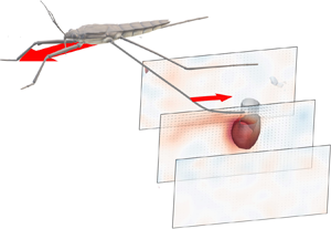
Additional considerations of the forces arising from such interface deformation are obviously required for the more complex locomotion at the air–water interface. During propulsion, late instar striders (figure 1a) push the surface of the water with their middle legs. These legs follow a semicircular trajectory in the horizontal plane, abruptly ending their course and leaving the surface. They deform the surface to a depth of 3 to 4 mm, which is of the order of the capillary length (2.7 mm), without breaking it (figure 1b). A leg pushes a much larger volume of water than itself and thus acts as a virtual oar made of leg-plus-dimple (figure 1b). The uniqueness of the water strider locomotion is due to the presence of this added mass of water, absent in most other organisms moving at the air–water interface, such as basilisk lizards and other invertebrates (Hsieh & Lauder Reference Hsieh and Lauder2004; Mukundarajan et al. Reference Mukundarajan, Bardon, Kim and Prakash2016).
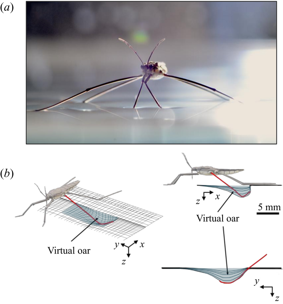
Figure 1. Water strider and virtual oar. (a) Photograph of Gerris palludum. (b) Illustration of the virtual oar geometry at  $t=27$ ms during sculling in perspective view and projected in the
  ${(x,z)}$ and
  ${(y,z)}$ planes. The virtual oar is the leg-plus-dimple that pushes a much larger volume of water than the leg itself.
Capillary waves, generated by the driving strokes of the legs, were first thought to be the primary hallmark of fluid motion forced by the water strider's legs (Andersen Reference Andersen1976; Denny Reference Denny1993; Suter et al. Reference Suter, Rosenberg, Loeb, Wildman and Long1997). However, Hu, Chan & Bush (Reference Hu, Chan and Bush2003) later showed that striders also produce a semi-annular vortex, with a momentum similar to that of the insect. This suggested the existence of a direct link between the momentum of the vortex and the momentum acquired by the insect. This finding enabled also the integration of the locomotion at the air–water interface into the then all-encompassing framework for animal locomotion (Dickinson Reference Dickinson2003). This integration was then questioned using numerical simulations (Gao & Feng Reference Gao and Feng2010). They showed that the pressure and viscous drag forces leading to the production of vortices were negligible relative to the capillary force, leading to the production of capillary waves (Gao & Feng Reference Gao and Feng2010). The singularity of this type of locomotion was reinforced through analytical modelling of the impulse transmitted by the insect; waves contributed 1/3 of the horizontal momentum, the remaining 2/3 coming from vortices (Bühler Reference Bühler2007). A recent extension to water finite depth and continuous leg forcing demonstrated the ability of such model to reproduce experimental recordings of precise water surface measurements (Steinmann et al. Reference Steinmann, Arutkin, Cochard, Raphaël, Casas and Benzaquen2018). More generally, previous studies regarding the mechanisms of arthropod propulsion at the air/water interface proposed a balance of the forces and momentum involved in the different processes (Suter et al. Reference Suter, Rosenberg, Loeb, Wildman and Long1997; Hu et al. Reference Hu, Chan and Bush2003; Bühler Reference Bühler2007; Gao & Feng Reference Gao and Feng2010; Rinoshika Reference Rinoshika2011). These studies follow two separate paths to estimate the forces balance, either a local balance of the force acting on the rowing leg or a wake measurement witnessing the momentum transfer, by characterizing the energy or momentum involved in both vortex and waves. We treat them in turns before focusing on the aims of our work.
1.1. Regarding the local force acting on rowing legs
In their experimental work on the surface propulsion of Dolomedes spiders, Suter et al. (Reference Suter, Rosenberg, Loeb, Wildman and Long1997) established that the resistance encountered by its rowing legs was due to three possible mechanisms. The first one is the standing bow wave generated by the movement of the leg, which balances the horizontal pressure of the leg against water. The second one is drag resistance, caused by the fluid viscous friction and by the difference in the fluid's pressure distributions along the leg. The third one is surface tension resistance due to the reconfiguration of the leg-cum-dimple and the resulting imbalance of capillary forces along the two contact lines on the leg. As the authors indicate, they did not proceed to the measurement of the actual predicted forces, but only provided mathematical relationships for the purpose of making testable predictions. They estimated that most of the resistance was caused by drag forces and not by surface tension, nor by the bow wave pressure. Gao & Feng (Reference Gao and Feng2010) were able to compute the different forces acting locally on a two-dimensional leg using finite-element numerical simulations of the interfacial flow during propulsion of water striders. They distinguished three terms that correspond to the contributions of pressure, viscosity and interfacial tension. Owing to the high spatial resolution of their numerical simulations, they were able to access local velocity gradients, normal pressure gradients and local surface gradients, all needed to estimate forces. They proved that the driving stroke delivers momentum from the leg to the water primarily through curvature and pressure forces. Their findings were orthogonal to ones of Suter et al. (Reference Suter, Rosenberg, Loeb, Wildman and Long1997), as they estimated that most of the resistance was caused by surface tension forces and not by drag forces nor by bow wave pressure. However, the three forces described by Gao & Feng (Reference Gao and Feng2010) and the three possible mechanisms highlighted by Suter et al. (Reference Suter, Rosenberg, Loeb, Wildman and Long1997) do not overlap. The contribution of interfacial tension is certainly equivalent in the two studies and the bow wave strength of Suter et al. can also be related to the increase of the normal pressure along the leg as defined by Gao & Feng (Reference Gao and Feng2010). The drag resistance of Suter et al. (Reference Suter, Rosenberg, Loeb, Wildman and Long1997) is, however, a combination of the pressure and viscous drag of the numerical study of Gao & Feng (Reference Gao and Feng2010). This lack of overlap of forces and mechanisms could partly explain the differences in the results of the two studies. Another source of discrepancies is the fact that they are not made at the same propulsion regime. Indeed, the leg velocity varies between 0.18 and 0.36 m s $^{-1}$ and diameters between 500
  $\mathrm {\mu }$m and 1.5 mm in Gao & Feng (Reference Gao and Feng2010), whereas Suter et al. (Reference Suter, Rosenberg, Loeb, Wildman and Long1997) study propulsion below 0.2 m s
 $^{-1}$ and at a fixed diameter of 1.5 mm.
1.2. Regarding wake measurements of the energy/momentum in the waves and vortices
In order to quantify the forces at play, other authors choose to study the wake resulting from the propulsion instead. In these studies, there are no estimation of the local forces acting on legs, primarily due to practical difficulties of experimentally measuring the flow close to the body of an animal (Dabiri Reference Dabiri2005). Hu et al. (Reference Hu, Chan and Bush2003) visualized the flow imparted to the water by the strider and roughly quantified its associated momentum. They estimated that the leg stroke produces a capillary wave packet, whose contribution to the momentum transfer is an order of magnitude less than the momentum of the strider. They highlighted the presence of two vortices and have estimated that the vortices transport most of the momentum. They also showed that waves and vortices travelled at different velocities. For an animal achieving a body velocity of  $100$ cm.s
 $^{-1}$, they estimated that the dipolar vortices translated backwards at a characteristic speed of
  $4$ cm.s
 $^{-1}$ and that the wave train had a phase speed of
  $30$ cm.s
 $^{-1}$. They concluded that the waves and the vortices were well separated in space and time. To explain this distribution of momentum transfer between waves and vortices, Bühler (Reference Bühler2007) modelled the impulse transmitted by the insect by the integral of a force localized in time and in space at a certain distance under the surface and oriented along a horizontal axis. The fact that the fluid was forced for a short time and in a compact region allowed him to use a linear theory, by neglecting the material derivative of the velocity compared to the forcing and pressure terms in Navier–Stokes equations. He characterized the fluid state at two times, at
  $t=0+$ immediately after the impulsive forcing, and at the adjustment flow time
  $t=+ \infty$, a sufficiently long time such that the surface waves have propagated away from the region of interest. He proved that the surface waves must carry away 1/3 of the horizontal momentum and 2/3 of the vertical momentum during the adjustment process (between
  $t=0+$ and
  $t=+ \infty$). Bühler (Reference Bühler2007) neglected the nonlinear interactions between the surface waves and the vortex. In his model, the air–water interface is not modified during the propulsion stage, but is pushed up by the vertical pressure established during the impulse generation below the surface. The quantification of the contributions of waves and vortices to the propulsion was also the focus of Gao & Feng (Reference Gao and Feng2010). They explained that curvature and pressure were the immediate origins of the propulsion force and that the partition of momentum between vortices and waves occurs later. They thereby highlighted the difficulty to formally separate the total momentum into one part due to the waves and another part due to vortices. The spatial division of regions with vortical and waves structure is indeed arbitrary. They distinguished vortex and wave regions in the late stage of the stroke and estimated that vortices carry about one third of the total momentum, a reversal of Buhler's estimate. Gao & Feng (Reference Gao and Feng2010) explained the divergence of their conclusions on partitioning with the one of Hu et al. (Reference Hu, Chan and Bush2003) by the geometrical differences between their respective studies. The rotation axis of the vortex appearing in Gao & Feng (Reference Gao and Feng2010) was parallel to the leg. They supposed that this vortex had a totally different origin from the hemispherical vortex dipoles of Hu et al. (Reference Hu, Chan and Bush2003). Indeed, Hu et al. (Reference Hu, Chan and Bush2003) and Rinoshika (Reference Rinoshika2011) have shown the presence of a pair of counter-rotating vortices at the ends of the dimple, which had a rotation axis perpendicular to the interface. Hu et al. (Reference Hu, Chan and Bush2003) supposed that this vortex dipole is present from the start of the rowing process, as it has been experimentally confirmed by Rinoshika (Reference Rinoshika2011).
The varying geometrical assumptions in these different studies leads to orthogonal conclusions and even to a lack of convergence in the identification of the mechanisms producing the observed vorticity. These orthogonal conclusions imply that an estimation of the applied forces – and thus the understanding of the propulsion mechanisms – remained beyond reach. Furthermore, the belonging of the strider locomotion to the general framework of animal locomotion is compromised. A definitive conclusion concerning the relative importance of capillary and drag forces can be reached only with time-resolved monitoring of all the local forces acting during propulsion. In particular, we need to understand the role of the virtual oar in the generation of vortical structures and in the recovery process of forces, a call made already earlier (Denny Reference Denny2004). This is our aim. We thus describe here the surface topography and vortical structure during the propulsion phase, as determined by tomographic particle image velocimetry in three dimensions (TomoPIV), which we complement with computational and mechanical leg models. Our numerical modelling and mechanical simulations are noticeably different from those provided by Gao & Feng (Reference Gao and Feng2010) and Suter et al. (Reference Suter, Rosenberg, Loeb, Wildman and Long1997). Regarding the modelling, we did not mechanically simulate the same size of leg as Suter et al. (Reference Suter, Rosenberg, Loeb, Wildman and Long1997), as we were focusing on tiny legs of water striders, contrary to Suter, who focused on the larger legs of Dolomede spiders. Regarding the numerical simulations, Gao & Feng (Reference Gao and Feng2010) did not numerically simulate tiny legs of 100 to 200  $\mathrm {\mu }$m diameter as we did. These two differences explain why they showed a larger contribution of pressure forces acting directly on the leg compared with curvature forces.
2. Methods
2.1. Experiments on freely moving animals
2.1.1. Animal collection
This study was conducted using the water strider Gerris paludum (figure 1a). We collected adult and larval stages from a freshwater pond in Tours, France (47 $^{\circ }$22’01.3”N–0
 $^{\circ }$41’29.5”E). The insects were kept in aquaria (
 $37 \times 17$ cm) at a constant temperature of
  $23 \pm 2^{\circ }\textrm {C}$, under a natural light cycle, until their use in experiments. The analysis was restricted to adults, as they generate large flow structures during their leg strokes.
2.1.2. TomoPIV set-up description
We performed Tomo-PIV measurements of freely moving animals at the water surface of a water tank (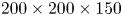 $200\times 200 \times 150$ mm) at 1000 frames s
 $^{-1}$. The measurement volume was located just below the surface (
 $30 \times 20 \times 10$ mm) and was visualized by four high-speed cameras (Phantom Miro 310) placed below the water tank (figure 2d). These four cameras acquired pictures at a rate of 1000 frame s
 $^{-1}$, with a resolution of
  $1280 \times 800$ pixels. They were mounted on ‘Scheimpflug’ optical mounts together with Nikon macro Lens (focal length 200 mm), ensuring focus on the entire plane. A fifth high-speed camera (Phantom V9.1,
  $1920 \times 1080$ pixels, 1000 f.p.s.) was placed on the top of the water tank and focalized on a larger measurement volume (
 $50 \times 90$ mm) to capture the movement of the whole insect's body. A pulsed laser (Photonics Industries DM30, 527 nm) illuminated the measurement volume via a custom light guide that included three mirrors and a cylindrical lens that expanded the beam in two axes to fit the size of the measurement volume. The laser was operated at high average power (25 W) and the pulse width was 24 ns. The enlarged beam went eventually through a diaphragm to avoid a decrease of light homogeneity in the periphery of the beam. The flow was seeded with 10
  $\mathrm {\mu }$m silver coated hollow glass particles (Dantec Dynamics, SHGS-10).
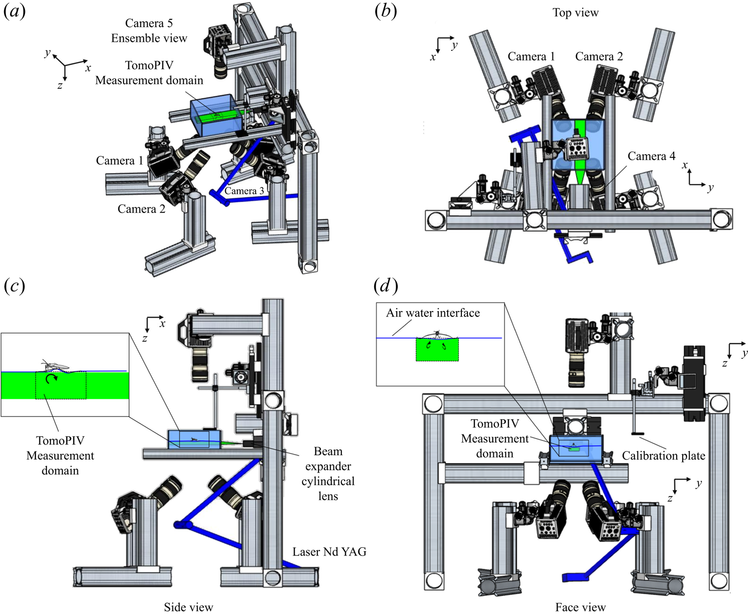
Figure 2. Four views of the experimental set-up of the TomoPIV. (a) Perspective view. (b) Upper view, projected in the  $(x,y)$ plane. (c) Side view in the
  $(z,x)$ plan with a focus on the position of both the insect and the measurement domain in the water tank. (d) Face view in the
  $(z,y)$ plan. The TomoPIV measurement domain is represented in green.
2.1.3. Local and wake measurements
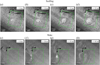
To ensure a high spatial resolution of the three-dimensional (3-D) velocity field, we choose a relatively small measurement volume. Such a small volume did not allow us to catch, in the same frame, both the local flow close to the water strider sculling leg and the flow in the wake of the strider. The TomoPIV measurements of the local and wake flows have thus been realized on different propulsions. TomoPIV was first used to study the temporal evolution of the surface topography and bulk flow during the ‘sculling phase’ as well as the ‘surface relaxation phase’, as described in the upper panels of figure 3. These three phases are described in detail later on. Figure 3 illustrates four instants of the movement of the whole insect's body, as taken by the fifth camera placed on the top of the water tank and focalized on a larger measurement volume ( $50 \times 90$ mm). The green rectangle represents the position of the TomoPIV measurement volume relative to the top camera view. We have also applied Tomo-PIV to the study of the 3-D vortical wake and waves patterns produced during the ‘wake phase’ after the stroke event. The main differences between the two experiments are the relative positions of the insect body and measurement volumes. In the ‘wake phase’ experiment the insect leg never crossed the TomoPIV measurement volume, but only brushed the side of this virtual volume, at 25 ms. The lower panels of figure 3 illustrate the relative locations of insect's body and measurement volume. The insect mass and maximal velocity were similar in the two experiments (
 $V= 0.7$ m s
 $^{-1}, m=30$ mg). From the successive images of figure 3, taken from above the water tank, we can guess the passing of an elongated circular surface wave, between 20 and 50 ms, as described in Steinmann et al. (Reference Steinmann, Arutkin, Cochard, Raphaël, Casas and Benzaquen2018).
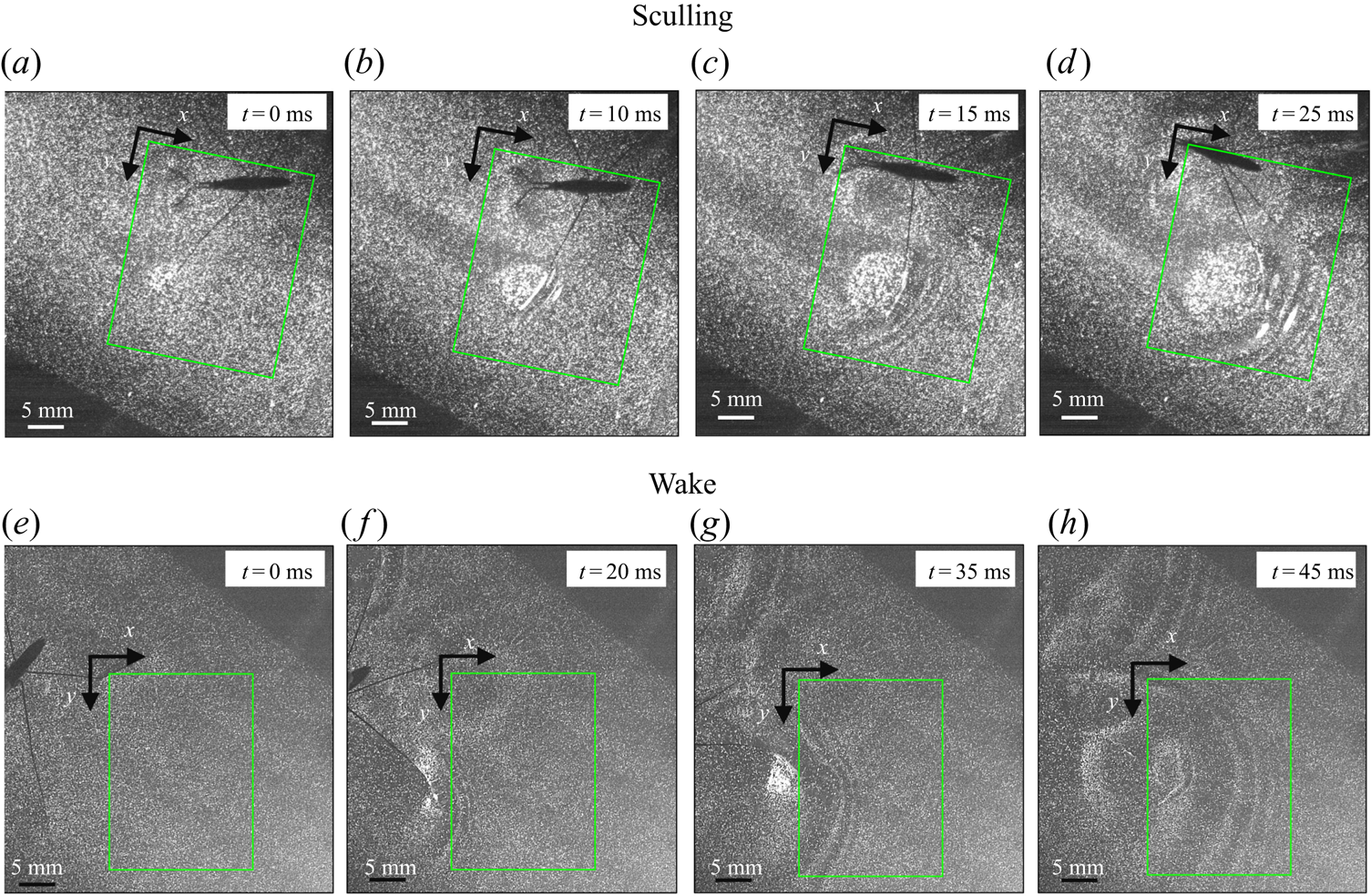
Figure 3. Relative locations of the TomoPIV measurement volume and rowing insect for the two experiments on strider propulsion. (a–d) Local flow close to the leg representing sequential images of the propulsion of a water strider Gerris palludum taken from above by camera 5, the ensemble view camera in figure 2(d), at four instants, 0 ms, 10 ms, 15 ms and 25 ms. The green rectangle shows the TomoPIV measurement volume. The leg sculls principally along the  $x$ axis. (e–h) Wave and flow in the wake representing sequential images of the wake behind the water strider at four instants, 0 ms, 20 ms, 35 ms and 45 ms.
2.1.4. Image acquisition and calibration procedure
The five cameras and the laser were synchronized by a high-speed controller (PTU-X, LaVision GmbH, Germany) and the image acquisition was controlled through DaVis software 8.4 (LaVision GmbH, Germany). The obtained images were first preprocessed, using sliding minimum subtraction, normalization with local average over  $300 \times 300$ pixels, Gaussian smoothing and sharpening of particles.
We performed an initial calibration of the four camera perspective, using four single views of a calibration plate for each camera (LaVision, Single sided dual plane calibration plate, model 058-5). It contained calibration markers on two depth levels, separated by 5 mm in the plane direction and by 3 mm in the out-of-plane direction. Using a micro positioner, we moved the calibration plate from the top to the bottom of the volume of measurement. For each of the four planes and for each of the images of the camera, we fitted a third-order polynomial calibration model with linear interpolation of the planes. In addition to this first calibration step, to ensure a correct estimation of velocities and to reduce the reconstruction errors due to unavoidable vibrations of the cameras, we performed a volume self-calibration for each measurement. This iterative procedure allowed us to minimize disparity errors associated with particle triangulation in the initial calibration (Wieneke Reference Wieneke2008).
2.1.5. Tomographic volume reconstruction, velocity field calculation and estimation of the interface position
From the four recorded camera images, we reconstructed the 3-D intensity distribution of the particles in the illuminated measurement volume. We used an iterative multiplicative algebraic reconstruction technique to produce a reconstructed  $30 \times 20 \times 10$ mm
 $^{3}$ volume, corresponding to
  $1000 \times 660 \times 500$ voxels with 30
  $\mathrm {\mu }$m voxel
 $^{-1}$. An example snapshot of this volumetric reconstruction is presented in figure S1(b–d). The reconstruction quality was enhanced by the use of a time-marching sequential motion tracking enhancement (SMTE) method (Novara & Scarano Reference Novara and Scarano2012). This iterative method reduces the energy lost into ghost particles during the algebraic reconstruction step. SMTE combines images from multiple consecutive exposures to enhance the reconstruction of individual intensity fields. The information from subsequent exposures is shared within the tomographic reconstruction process of a single object (Novara & Scarano Reference Novara and Scarano2012). Then, the interrogation areas, corresponding to sub-volumes of
  $64\times 64 \times 64$ voxels, were cross-correlated to obtain the three-dimensional velocity fields, with an inter-frame time of 1 ms. Using a 75 % overlap, the interrogation volume provided a spatial resolution in all three directions of 0.48 mm. The velocity field was post-processed using a local median filter with
  $3 \times 3 \times 3$ vector neighbourhoods. This resulted in approximately
  $23 \times 10^{4}$ (
 $110 \times 70 \times 30$) grid points for each time step, as illustrated in figure S1(e–g). In the following representations of the bulk flow, we show surfaces of iso-vorticity, typically used to highlight the presence of coherent structures. The vorticity is estimated using spatial derivative. The spatial derivation tends to increase the local noise in the measurement field to prevent a correct and continuous estimation of the isosurfaces. The local vorticity used to represent the isovorticity surface has therefore been computed on spatial-averaged velocity fields.
Despite the use of the self-calibration procedure and the use of SMTE, we could not prevent the production of ghost particles during the algebraic reconstruction procedure. Ghost particles are notably produced during the reconstruction of the flow above the water surface, where we know particles are absent. The presence of these unwanted particles results in a significant increase of error during the cross-correlation phase. Luckily, seeding particles tend to agglomerate on the water surface. This increase of particle density is visible in figure S1(a–c). The consequential increase of particle density at the water surface thus allowed us to precisely determine the position of the interface in multiple cross-sections of the reconstructed volume. For each time step, we used this result to produce of a 3-D mask that followed the topography of the interface and masked the portion of the unwanted reconstructed area, avoiding thereby the incorporation of ghost particles. These steps allowed us to eventually produce a complete representation of the time-resolved surface topography  $\zeta (x,y,t)$, leg position and flow velocity field
  $\boldsymbol {u}$ (Figure S1e–g).
2.2. Mechanical simulations
2.2.1. Set-up description
We describe here the experimental set-up of a physical model of a leg moving at the air–water interface. The experiments were carried out in a rectangular water tank ( $20 \times 20 \times 15$ cm) (figure 4a). We simulated the water strider leg using a cylinder (
 $D=0.1$ mm,
  $L=40$ mm, figure 4b) made of steel, of identical diameter and similar length to real animals (Koh et al. Reference Koh, Yang, Jung, Jung, Son, Lee, Jablonski, Wood, Kim and Cho2015; Steinmann et al. Reference Steinmann, Arutkin, Cochard, Raphaël, Casas and Benzaquen2018). It has been shown that the leg may undergo a large deformation while pushing on the air–water interface (Ji, Wang & Feng Reference Ji, Wang and Feng2012). The curved shape of the mechanical leg was chosen to mimic the deformed shape of the tarsi. This shape, which marries the curvature of interface, greatly reduces the forces exerted on the air–water interface and prevents its breaking while sculling at high velocity. The surface was furthermore covered with a super-hydrophobic coating (Ultra ever Dry, TAP France, Plaisir), which reproduced the hydrophobic characteristic of natural legs and allowed us to reach a contact angle of 175
 $^{\circ }$, very close to the 168
 $^{\circ }$ of Gerris legs (Gao & Jiang Reference Gao and Jiang2004; Feng et al. Reference Feng, Gao, Wu, Jiang and Zheng2007). The mechanical leg was held by a micromanipulator (Newport M-MT-AB2) placed on a horizontal translation stage (LAL35, Cedrat Technologies, Meylan, France) and positioned in contact with the water surface. The translation stage, allowing a precise movement along the
  $x$ axis, was connected to a high-speed controller (LAC-1, Cedrat Technologies, Meylan, France) driven by a computer. Both the acceleration and velocity of the piston were controlled with high precision (
 $\pm$4 %) and the mean distance to reach a constant speed was set to 1 cm. We have restricted our experiment to 1-D displacements at fixed depth. The experimental set-up allowed us to independently set both velocity and depth of propulsion of the mechanical leg. We explored leg velocities ranging from 20 to 72 cm s
 $^{-1}$ and depths ranging from 600
  $\mathrm {\mu }$m to 3 mm, to cover the range of velocities and depths of water striders (Hu et al. Reference Hu, Chan and Bush2003; Hu & Bush Reference Hu and Bush2010; Steinmann et al. Reference Steinmann, Arutkin, Cochard, Raphaël, Casas and Benzaquen2018). We thus produced a matrix of experiments in the ‘speed–depth’ parameter space (figure 5). For the analysis, we only kept the experiments for which the interface did not break after 30 ms of movement.
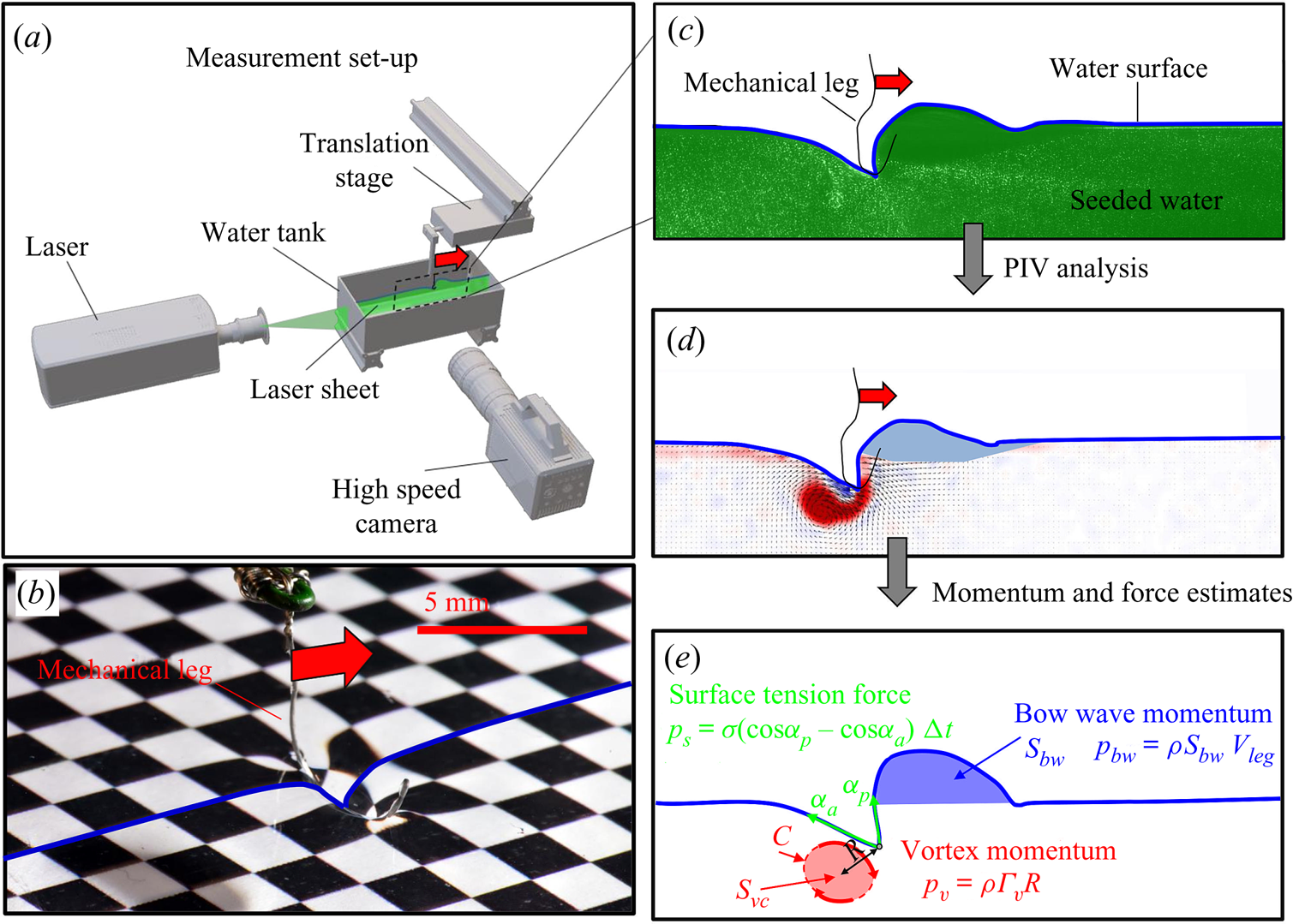
Figure 4. (a) Experimental set-up of the mechanical simulation of a sculling leg. The mechanical leg is guided by a translation plate. The previously seeded flow and the air–water interface are illuminated by a laser sheet. The visualization of the temporal evolution of the topography of the interface and of the flow are carried out with the aid of a high-speed camera, placed perpendicularly to the laser plane. (b) Photography of the mechanical leg pushing down the air–water interface statically. A micromanipulator, placed on the translation plate, allows us to precisely position the leg on the interface. The static leg initially exerts pressure on the interface creating a meniscus. The blue line figures out the vertical cross-section of the initial deflection of the air–water interface. (c) Snapshot of the vertical cross-section of the seeded water flow and of the surface, as obtained by the high-speed camera. (d) Vertical cross-section of the velocity field obtained from PIV analysis and surface profile. (e) Diagram of the capillary force integrated over time and of the two potential hallmarks of momentum transfer during propulsion of a leg at the interface: the bow wave momentum and the vortex momentum.
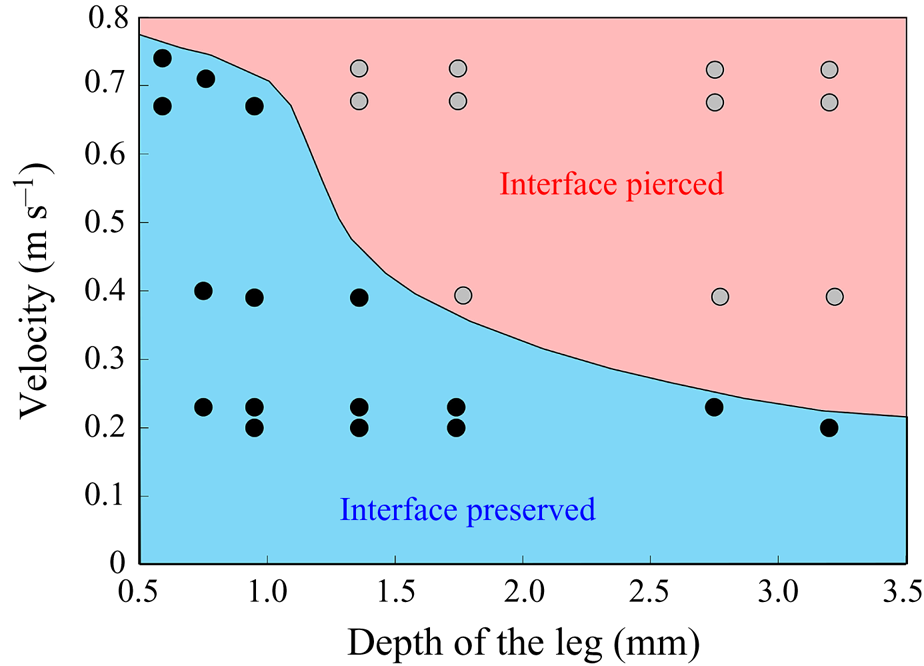
Figure 5. Matrix of experiments with a mechanical leg in the velocity–depth parameter space. The filled points represent the velocity–depth values for which the interface remained unbroken for at least 30 ms after the start of the stroke. The empty points represent the experiments for which the interface broke prematurely.
2.2.2. Two-dimensional PIV and estimation of the surface topography
Flow measurements were performed using 2-D PIV on water seeded with 10  $\mathrm {\mu }$m glass particles (Dantec Dynamics, SHGS-10). The continuous laser (CNI, MGL-F, 532 nm, 2W) illuminated the flow produced by the leg displacements through the glass (figure 4a). The laser beam was transformed in a laser sheet (width=17 mm, thickness = 2 mm) through a cylindrical lens. A target area was then imaged onto the CCD array of a high-speed digital camera (figure 4c) (2000 f.p.s.,
  $1632 \times 600$ px Vision Research Phantom 9.1) using a NIKON lens (Micro Nikor
  $f=50$ mm) that produced a
  $36 \times 14$ mm window around the moving artificial leg. The 2-D velocity vector fields were derived from sub-sections of the target area of the particle-seeded flow by measuring the movement of particles between two images (
 ${\rm \Delta} t = 500~\mathrm {\mu }$s) (figure 4d). Images were divided into small subsections (width, 700
  $\mathrm {\mu }$m; resolution,
  $32 \times 32$ pixels; covering rate, 75 %) and cross-correlated with each other using a commercial PIV software (Lavision Davis 8.3). The correlation produced a signal peak, identifying the common particle displacement. An accurate measurement of the displacement (and thus of the velocity) was achieved with subpixel interpolation (figure 4d). The surface topography was manually estimated on PIV images.
2.2.3. Quantification of local forces acting on legs and of momentum transfer
The strength of propulsion at the air–water interface depends on the ability of the rowing leg to create resistance to its motion. Our set-up and images allowed us to estimate the primary resisting force, which is the interface resistance or capillary force. It represents the surface tension force experienced at the anterior and posterior margins of the leg and it results in a horizontal net force per unit length. This force can be assessed by the estimation of the dissymmetry of the two contact lines on the leg meniscus around the leg and is equal to
 \begin{equation} F_s=\sigma (\cos {\alpha }_p-\cos {\alpha }_a), \end{equation}
with  $\sigma$ being the air–water interface surface tension (72,8.10
 $^{-3}$ N m
 $^{-1}$) and
  ${\alpha }_p$ and
  ${\alpha }_a$, the posterior and anterior relative angles of the meniscus, respectively (figure 4e). These two angles are estimated on the images of vertical cross-sections of the water surface. To obtain momentum, we integrated this force over time
  ${\rm \Delta} t$
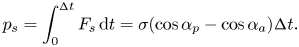 \begin{equation} p_s=\int_0^{{\rm \Delta} t} F_s \, {\textrm{d}}t =\sigma (\cos {\alpha }_p-\cos {\alpha }_a){\rm \Delta} t. \end{equation}
We also estimated the force carried by the two distinctive hallmarks of momentum transfer between the leg and the water. The first phenomenon that witnesses an exchange of momentum is the presence of a bow wave. As the leg moves with a sufficiently large velocity at the interface, it generates a bow wave, resisting to its forward motion. The momentum transfer, per unit length (kg s $^{-1}$), associated with this mechanism was estimated as that necessary to move the cross-section surface
  $S_{bw}$ of density
  $\rho _{water}$ to the speed of the leg
 \begin{equation} p_{bw}=\rho_{water}S_{bw}V_{leg}. \end{equation}
Using PIV images, we estimated  $S_{bw}$ as the area situated above the surface static resting depth
  $z=0$ (figure 4e).
The second witness of a momentum transfer is the emission of a vortex. The strength of the vortex is determined using circulation,  $\varGamma _v$ (m
 $^{2}$ s
 $^{-1}$) (figure 4e). It is the line integral of the tangential velocity component
  $\boldsymbol {u}$ about a curve
  $C$ enclosing the vortex core surface (
 $S_{vc}$) (Batchelor Reference Batchelor1967). This circulation can be related to vorticity
  $\boldsymbol{\omega}$ by Stokes’ theorem
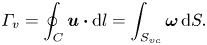 \begin{equation} \varGamma_v=\oint_C\boldsymbol{u} \boldsymbol{\cdot} {\textrm{d}}l=\int_{S_{vc}}\boldsymbol{\omega} \, {\textrm{d}}S. \end{equation}
The optimal surface of the vortex core  $S_{vc}$ is estimated by increasing the integration surface until an asymptotic value of circulation is attained. It represents the vortex's total circulation (Willert & Gharib Reference Willert and Gharib1991). In two dimensions, the momentum of the vortex
  $p_v$ is given by
 \begin{equation} p_v=\rho \varGamma_v R, \end{equation}
where  $\rho$ (kg m
 $^{-3}$) is the water density and
  $R$ (m) is the distance between the vortex centre and the water surface. Here,
  $p_v$ is a momentum per unit length (leading to kg s
 $^{-1}$). We chose this formulation for its dimensionality, to be able to compare the amplitude of the vortex momentum with the amplitude of the momentum of the bow wave, which is also expressed per unit length.
2.3. Numerical simulations
We have numerically computed the interfacial flow during the sculling of a leg using finite-element simulations. Our numerical simulations are validated with the results of the 2-D PIV experiments with a mechanical leg, to confirm the regime of successful locomotion and to quantify the forces involved in these different regimes.
2.3.1. Physical model of the air–water interface
We modelled the air–water interface as a diffuse interface (Yue et al. Reference Yue, Feng, Liu and Shen2004, Reference Yue, Zhou, Feng, Ollivier-Gooch and Hu2006; Gao & Feng Reference Gao and Feng2010) using the phase field method implemented in Comsol Multiphysics 5.3 (COMSOL, Inc![]() ). In this method, the interfacial layer is governed by a phase field variable with
). In this method, the interfacial layer is governed by a phase field variable with  $\phi$ (
 $\phi =-1$ in the water and
  $\phi =1$ in the air);
  $\phi$ varies in a smooth way across the interface, which is given by the level set
  $\phi =0$. We can express the concentration density
  $\rho$ (kg/m
 $^{3}$) and viscosity
  $\mu$ (Pa.s) as a function of
  $\phi$
 \begin{equation} \rho =\tfrac{1}{2}(1-\phi ){\rho }_{water}+ \tfrac{1}{2}(1+\phi ){\rho }_{air}, \mu =\tfrac{1}{2}(1-\phi ){\mu }_{water}+ \tfrac{1}{2}(1+\phi ){\mu }_{air}. \end{equation}
The interface has a small but finite thickness in which the two fluids are mixed and store some mixing energy. According to Cahn & Hilliard (Reference Cahn and Hilliard1958), the mixing energy, or chemical potential  $G$, can be expressed as the sum of (i) a bulk energy (
 ${-\lambda \nabla }^{2}\phi$), reflecting the total separation of the two phases, i.e. the phobic aspect and (ii) a philic effect
 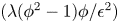 $({\lambda ({\phi }^{2}-1)\phi }/{{\epsilon }^{2}})$ expressing the total mixing of the two phases
 \begin{equation} G=\lambda [-{\nabla}^{2}\phi +({\phi }^{2}-1)\phi /\epsilon^{2}], \end{equation}
where  $\lambda$ is the mixing energy (N) density and
  $\epsilon$ (m) is the capillary width characterizing the thickness of the diffuse interface. They are related to the surface tension
  $\sigma$ (N m
 $^{-1}$) by
 \begin{equation} \sigma =\frac{2\sqrt{2}}{3}\frac{\lambda }{\epsilon }. \end{equation}
This is a simplified expression of the free energy, as we neglected additional sources of energy. The profile of the phase field variable across the interface is determined by the competition of the two philic and phobic effects. We modelled the forcing of the flow field on the interface represented by introducing the advective Cahn–Hilliard equation (Cahn & Hilliard Reference Cahn and Hilliard1958). This transport equation describes the evolution of  $\phi$ in a flow field
  $\boldsymbol {u}$
 \begin{equation} \frac{\partial \varPhi}{\partial t}+\boldsymbol{u} \boldsymbol{\cdot} \boldsymbol{\nabla}\varPhi=\boldsymbol{\nabla}\boldsymbol{\cdot}(\gamma \boldsymbol{\nabla }G), \end{equation}
where  $\gamma$ is the mobility. The flow velocity field
  $\boldsymbol {u}$ transports the phase field variable through convection. The flow field can be determined by solving the Navier–Stokes equations. The surface tension is incorporated into the equation of momentum as a body force normal to the interface by multiplying the chemical potential of the system
  $G$ with the gradient of the phase field variable
  $\boldsymbol {\nabla }\phi$. We considered the fluid as incompressible, so the flow is governed by the incompressible Navier–Stokes equations (continuum and momentum equations)
 \begin{gather} \rho \boldsymbol{\nabla} \boldsymbol{\cdot} \boldsymbol{u}=0, \end{gather}
 \begin{gather}\rho \frac{\partial \boldsymbol{u}}{\partial t}+\rho \boldsymbol{u}\boldsymbol{\nabla }\boldsymbol{u}=\boldsymbol{\nabla} \boldsymbol{\cdot}[{-}p\boldsymbol{I}+\mu (\boldsymbol{\nabla }\boldsymbol{u}+{\boldsymbol{\nabla }\boldsymbol{u}}^{T})]+G\boldsymbol{\nabla }\varPhi-\rho {g}. \end{gather}
Along the wetted cylinder, the contact angle for the fluid  ${\theta }_w$ is specified, giving the following contact angle boundary condition:
 \begin{equation} \boldsymbol{n} \boldsymbol{\cdot} {\epsilon }^{2}\boldsymbol{\nabla}\phi ={\epsilon }^{2}\cos ({\theta }_w)|\boldsymbol{\nabla}\phi |. \end{equation}
Across the wetted cylinder, the mass flow is zero, as described by the following equation:
 \begin{equation} \boldsymbol{n}\boldsymbol{\cdot} \boldsymbol{\nabla} G=0. \end{equation}
We finally imposed the leg velocity along the wetted cylinder surface, together with a no-slip boundary condition, as
 \begin{equation} \boldsymbol{u}=(U_{leg},V_{leg}). \end{equation}
2.3.2. Numerical methods
The parameter values of the simulations are given in the SI Table S1. We used the capillary length (2.7 mm) as characteristic length to express our dimensionless numbers. The equations were solved using the finite elements method (FEM) multiphysics coupling software Comsol 5.3. The problem was solved in a rectangular domain of size  $80 \times 11$ mm (figure 6). We used an adaptative moving meshing method that allows us to refine the mesh up to 10
  $\mathrm {\mu }$m elements size close to the cylinder. This minimal size of a mesh element is lower than the minimal diffuse interface thickness in order to maximize the convergence in the numerical resolution of the Cahn–Hilliard equation. The cylinder size was set to 200
  $\mathrm {\mu }$m. It is thus larger than the diameter of the mechanical leg used in our experiments (100
  $\mathrm {\mu }$m). As explained by Gao & Feng (Reference Gao and Feng2010), computing thinner legs becomes computationally very costly, as it would require a thinner diffuse interface to approach the sharp interface limit. We discuss the differences in leg diameter between mechanical and numerical simulations later in the discussion section. The moving mesh feature of COMSOL 5.3 was used to impose a movement to the cylinder surface. We coupled two methods for solving both the laminar incompressible flow and the position of the moving interface. Using the laminar flow method, we solved the Navier–Stokes equation describing the laminar incompressible flow. Using the phase field method, we solved the advective Cahn–Hilliard equations allowing us to track moving interfaces. As the problem is unsteady, we used a time-dependent solver, MUMPS (multi massively parallel sparse direct solver, Amestoy et al. Reference Amestoy, Duff, Koster and L'Excellent2001) to solve the sparse linearized equation system. We imposed a zero flow field in both air and water as initial conditions. The initial and static shape of the equilibrium interface was determined by the force balance between interfacial tension and hydrostatic pressure. We set this shape by slowly moving down the wetted cylinder to the nominal depth of stroke
  $h_l$ as defined in the experimental study. It formed a symmetric dimple, whose lateral extent is characterized by the capillary length
  $l_c$ (figure 6).
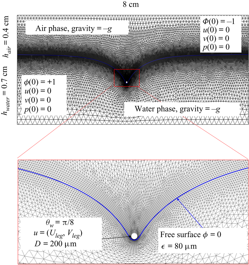
Figure 6. Numerical simulation. Typical meshing with refinement around the leg and the air–water interface. The aspect ratio of the figure does not match the real one ( $80 \times 11$ mm). The state shown here represents the initial condition of the equilibrium interface for a depth of stroke
  $h_l = 3$ mm. The free surface is represented in blue in the inset and its location is numerically determined where the phase field variable
  $\phi = 0$.
2.4. Force balance and energy estimation
Following the theoretical developments of Hu & Bush (Reference Hu and Bush2010) and Gao & Feng (Reference Gao and Feng2010), we have estimated the rate of change of momentum acting on a leg. This net force acting on the leg is given by
 \begin{equation} {\boldsymbol{F}}_{\boldsymbol{leg}}= M\boldsymbol{g}+{\boldsymbol{F}}_{\boldsymbol{s}}+ {\boldsymbol{F}}_{\boldsymbol{p}}+{\boldsymbol{F}}_{\boldsymbol{v}}, \end{equation}
where  $M\boldsymbol {g}$ is the insect weight supported by the leg,
  ${\boldsymbol {F}}_{\boldsymbol {s}}=\int _C{\sigma \boldsymbol {t}\, {\textrm {d}}C}$ is the capillary force on the contact line of the leg
  $C, {\boldsymbol t}$ is the surface tangent vector at the contact line,
  ${\boldsymbol {F}}_{\boldsymbol {p}}=\int _{\mathit {\varSigma }}{p\boldsymbol {n}\, {\textrm {d}}S}$ is the pressure stress on the leg surface
  $\varSigma , {\boldsymbol n}$ is the surface normal vector and
  ${\boldsymbol {F}}_{\boldsymbol {v}}=\int _{\mathit {\varSigma }}{\mu [{\boldsymbol {\nabla } }\boldsymbol {u}+{[{\boldsymbol {\nabla } }\boldsymbol {u}]}^{T}]\boldsymbol {n}\, {\textrm {d}}S}$ is the viscous stress on the leg surface, with
  $\boldsymbol {u}$ being the velocity field and
  $\mu$ the dynamic viscosity. Hu & Bush (Reference Hu and Bush2010) prove that, in the parameter regime of most water-walking arthropods, the capillary force dominates the pressure and viscous drags (
 $F_s \gg F_p \gg F_v$), so that
 \begin{equation} {\boldsymbol{F}}_{\boldsymbol{leg}}=\int_C{\sigma \boldsymbol{t}\, {\textrm{d}}C}+M\boldsymbol{g}. \end{equation}
 We supposed that the energy transfer results in a deformation of the surface and in a water displacement, during the sculling of the leg at the interface. The deformed interface gains an energy  $E_s(t)$ and the fluid gains a kinetic energy
  $E_k^{f}(t)$. The energy of the surface is the sum of its curvature energy (first term in the right-hand equation (2.17)) and its gravitational energy (second term in the right-hand equation (2.17)) and is given by
 \begin{equation} E_s(t)=\tfrac{1}{2}\sigma \int{{\textrm{d}}x\, {\textrm{d}}y{|\boldsymbol{\nabla} \zeta (t,x,y)|}^{2}}+\tfrac{1}{2}\rho g\int{{\textrm{d}}x\, {\textrm{d}}y}\zeta^{2} (t,x,y)-E_s(0), \end{equation}
where  $\zeta (t,x,y)$ (m) is the time-resolved air–water interface position,
  $\boldsymbol {\nabla }\zeta (t,x,y)$ is the surface gradient and
  $E_s(0)$ is the energy of the statically deformed interface at
  $t=0$. The curvature energy corresponds to the change in interface area compared to the resting flat interface area, multiplied by surface tension
  $\sigma =72,8.10^{-3}$ J m
 $^{-2}$. We furthermore supposed that some energy is also transferred to the fluid in the form of fluid kinetic energy
  $E_k^{f}(t)$
 \begin{equation} E_k^{f}(t)=\tfrac{1}{2}\rho\int_{V_c}{{\textrm{d}}x\, {\textrm{d}}y\, {\textrm{d}}z{\boldsymbol u}(x,y,z,t)^{2}}. \end{equation}
With  ${\boldsymbol u}(x,y,z,t)$ being the water velocity field.
3. Results
3.1. Experiments with living animals
In this section, we present our results concerning the measurements on freely moving animals, first starting with a description of the 3-D movement of the sculling leg. We then analyse the surface topography and the bulk flow at three key phases of the propulsion, (i) the sculling phase, (ii) the surface relaxation phase and (iii) the wake phase. After the qualitative description of these three phases, we conduct a momentum and energy analysis.
3.1.1. Three-dimensional movement of the leg
We have characterized a typical trajectory of a water striders propulsive leg (figure 7). During its propulsion, a water strider pushes the surface with the median legs to the point of deforming it very strongly. The force emitted by the insect has both a horizontal and a vertical component. The insect can bend this interface to a depth of 3 to 4 mm without breaking it. In the frame of reference of the body of the insect, the median leg pushes backwards and downwards, remains fixed in this position for a while before returning to its initial position. In the frame of reference of the fluid, the leg by contrast changes abruptly directions, at the end of its course, to follow the movement initiated by the body. In the vertical  $(x,z)$ plane, the leg gradually pushes the surface without breaking and then rises sharply while leaving the surface (figure 7). At the same time, on the surface, the leg follows a pseudo-circular trajectory in the horizontal
  $(x,y)$ plane. The tarsi deform during propulsion along a curve matched by the rounded shape of the meniscus.
Figure 7. Three-dimensional movement of the sculling leg of the water strider. Successive locations of the water strider's leg in the  $(x, y), (x, z)$ and
  $(y, z)$ planes. At 0 ms, the middle leg (in green ) begins its sculling movement. At 20 ms, it reaches its maximal depth (in blue). It then continues its trajectory, leaving the water at 30 ms (in red). The intermediate positions between these three instants are shown in grey. The two black dotted lines represent the trajectories of two extremities of the tarsal segments of the leg in contact with the air–water interface. The arrows on the lines indicate the directions of displacement.
3.1.2. Description of the flow and the air–water interface
We first describe the local flow close to the leg during the onset of the interaction between the leg, the interface and the bulk flow. Named sculling phase, it is illustrated by the four sequential images of figure 3(a–d). The TomoPIV analysis of the flow velocity and surface deformation are in the panels (a.i), (a.ii) and (a.iii) of figure 8. The leg pushes down, creating an increasing depression of the free surface. The energy contained in the deformed surface increases over time (figure 8a.i and figure 10a). The interface is rapidly displaced by the leg. This displacement of the water surface establishes the boundary conditions between air and the underneath fluid. There is an immediate generation of vorticity, as seen by the two vortices in the  $(x,y)$ plane (figure 8a.iii). The vortex also develops under the interface (figure 8a.ii) in the
  $(x,z)$ plane. According to Helmholtz's theorem, a vortex line cannot start or end in the fluid (Kundu et al. Reference Kundu, Cohen, Dowling and Tryggvason2015), but must end either at a solid boundary or form a closed loop. In our particular case, it ends at the boundary of the fluid. Thus these apparent three vortices form in fact a single semi annular vortex, visible in the 3-D representation of the isosurface of vorticity (figure 8a.i). The vortex geometry is related to the dimple geometry and closely follows the displacement of the dimple. The vorticities, circulations and velocities are large in both horizontal and vertical plane, the vortex being flattened in the horizontal plane.
Figure 8. Dynamics of surface topography and bulk flow at two instants, during the sculling phase (a.i), (a.ii) and (a.iii) as well as the surface relaxation phase (b.i), (b.ii) and (b.iii). (a.i) Three-dimensional snapshot representation of body position, surface topography and vorticity isosurface in the underlying fluid during the sculling phase ( $\vert \omega \vert =150$ s
 $^{-1}$ at
  $t=20$ ms). The leg curving the interface is shown in red. The blue line represents the x-axis cross-section of the surface at
  $y=0$. (a.ii) Vertical cross-section of the air–water interface and the flow velocity field. This cross-section is located on a line crossing the middle of the leg. The position of the leg is indicated in red, and the blue line shows the local elevation of the water surface along a plane crossing the middle of the leg tarsi. The green area is the isosurface of vorticity along the
  $y$ axis. The vertical circulation of the vortex (
 $\varGamma _v$) is estimated by integrating the vorticity over this area. The radius of the semi-annular vortex is defined as the distance between the leg and the vortex core. (a.iii) Flow velocity field in the fluid at the interface. The estimated position of the leg is indicated as a dotted red line. The two counter-rotating cylinders typical of a dipolar vortex are visible. The red area is the isosurface of vorticity along the
  $z$ axis. The vertical circulation of the two vortices (
 $\varGamma _h-$ and
  $\varGamma _h+$) was estimated by integrating the vorticity over the surface flow. (b.i) Snapshot of body position, surface topography and isosurface of vorticity in the underlying fluid during the wave relaxation phase (
 $\vert \omega \vert =150$ s
 $^{-1}$ at
  $t=35$ ms). (b.ii) and (b.iii) are similar to (a.ii) and (a.iii), except that the leg has been lifted from the surface.
At some 30 ms, the leg leaves the free surface and the interface relaxes and recovers its horizontal nature (figure 8b.ii). This is the surface relaxation phase. The vertical velocity of the beforehand strongly depressed part of the interface is now large enough to pull up the fluid (figure 8b.ii). It results in an increase of the vertical velocity of the fluid, visible in the vertical cross-section of figure 8(b.ii). At the same time, the bow wave spreads on the surface and pushes the fluid down, as shown in figure 8(b.ii). The two phenomena result in an increase of the vorticity in the vertical plane (horizontal vorticity along  $y$ axis) (figure 10a). At the same time, the vorticity in the horizontal plane (vertical vorticity along
  $z$ axis) decreases (figure 8b.iii and figure 10a). The leg does not produce any thrust once lifted, so that the decay of the vorticity in the
  $(x,y)$ plane is mostly due to the viscous diffusion of the translating vortex ring in the otherwise immobile fluid.
The measurements presented above are carried out close to the leg. Thus they do not allow us to quantify the energy radiated by the waves, as they have already left the measurement domain. We therefore present here the TomoPIV study of the 3-D flow and waves patterns produced in the wake of a water strider leg during the wake phase. This phase is illustrated by the sequential images of the propulsion in figure 3(e–h). The main difference between these measurements and the previous ones is the relative position of the insect body and measurement volume. Here the insect leg never crosses the TomoPIV measurement volume. The leg only brushes the side of the virtual volume at  $t=25$ ms. This explains the lack of particles movement monitored before 20 ms. We exhibit the flow velocity in the water at two instants after the leg stroke of the water strider in figure 9(a,b). Figure 9(a) illustrates the relative position of insect body, legs and measurement volume in its frame of reference. We illustrate the passage of the wave at 40 ms in figure 9(a). The wake phase thus starts when the surface relaxation phase ends but also extends in a much larger spatial volume than the first two phases.
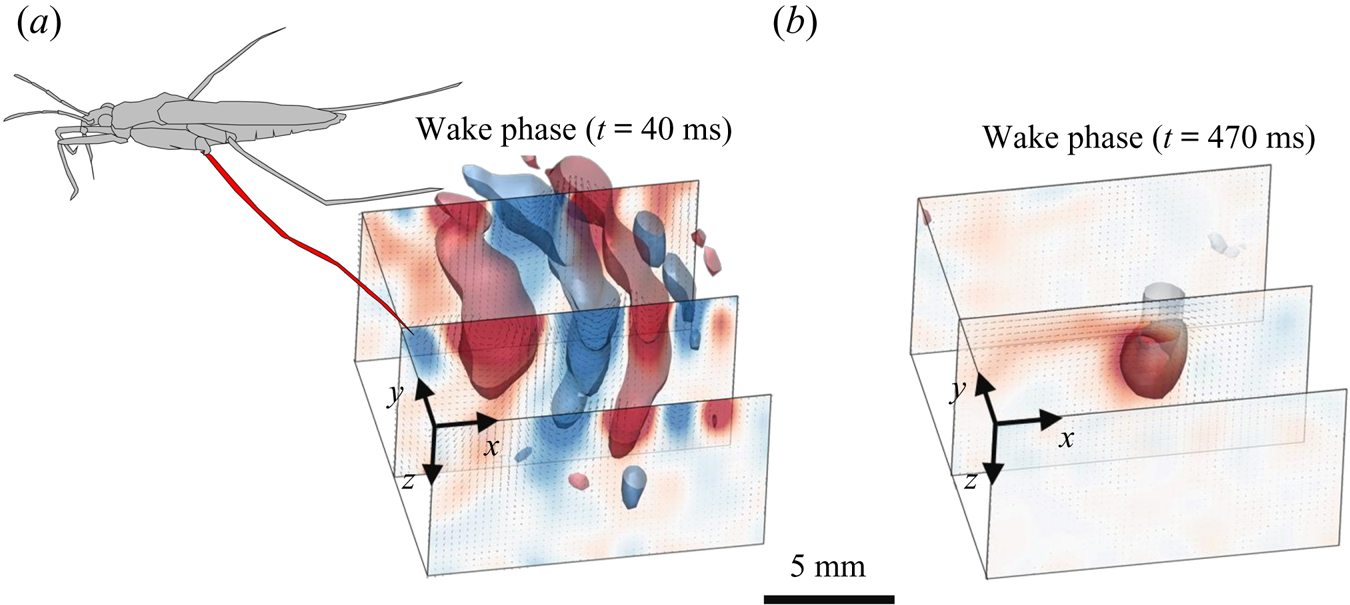
Figure 9. (a) Water bulk dynamics in the wake, after water strider propulsion during the passage of the wave. Relative positions of the insect and measurement volume at  $t=40$ ms. The cross-sections of the velocity field along the
  $(x,z)$ planes are represented at 3 locations along y axis. The isosurface colours correspond to the vorticity along
  $y$, in blue
  $\omega _y=-20\ \textrm {s}^{-1}$ and in red
  $\omega _y=20\ \textrm {s}^{-1}$. (b) Visualization of the convection of the semi-annular vortex at
  $t=470$ ms. The water strider then leaves the field of view. The isosurface colours correspond to the absolute vorticity in red
  $\vert \omega \vert =12\ \textrm {s}^{-1}$.
As we can observed in figure 9(a), the particles follow a circular clockwise motion during the passing of a surface wave, from a Lagrangian point of view. However, PIV technique gives information about the instantaneous velocity field, so that, from an Eulerian point of view as the one adopted in PIV analysis, this clockwise motion appears as a succession of clockwise and counter-clockwise vortices. This is also shown, for instance, in the work of Umeyama (Reference Umeyama2012), who carried out an Eulerian–Lagrangian analysis of particles velocities of a wave motion using PIV. The amplitude of motion decreases with increasing water depth. The wave phase velocity is estimated at  $c_p=34$ cm s
 $^{-1}$, implying that the wave train travels through the 2 cm long volume in less than 60 ms. The particle movement has a zero mean velocity during the passing of the wave. At
  $t=40$ ms, the semi annular vortex is not visible yet, as it is detaching from the leg outside of the measurement volume. Later, the semi-annular vortex travels through the measurement volume with a much lower convection velocity of
  $V_{vortex}=2.8$ cm s
 $^{-1}$ (figure 9b).
3.1.3. Momentum and energy analyses
In the following sections, we proceed to the analysis of the momenta imparted to the vortex and to the wave, during the propulsion. However, to estimate correctly their respective momenta, we have to choose a somewhat arbitrary spatial boundary between vortex and bow wave location. We agree with Gao & Feng (Reference Gao and Feng2010) that the vortex and the bow wave regions are in fact inseparable, when estimating momentum in the fluid. Furthermore, the very concept of interface momentum is questionable, as an interface has no momentum because it carries no mass. Dissociating momentum in fluid bulk and wave motions being thus difficult, one can rather focus on the energy necessary for the displacement of the fluid bulk and that necessary for the displacement and the deformation of the interface.
During the sculling phase, the leg movement at the interface results in the deformation of the surface, which gains a potential energy  $E_s(t)$ composed of gravitationnal and curvature energy, which can be computed using (2.17). The surface energy reaches a maximum of
  $E_{smax}=10^{-6}\ \textrm {J}$ around 25 and 30 ms (figure 10a). At the same time, the leg produces a bulk flow characterized by the emission of a semi-annular vortex whose circulation changes with time.
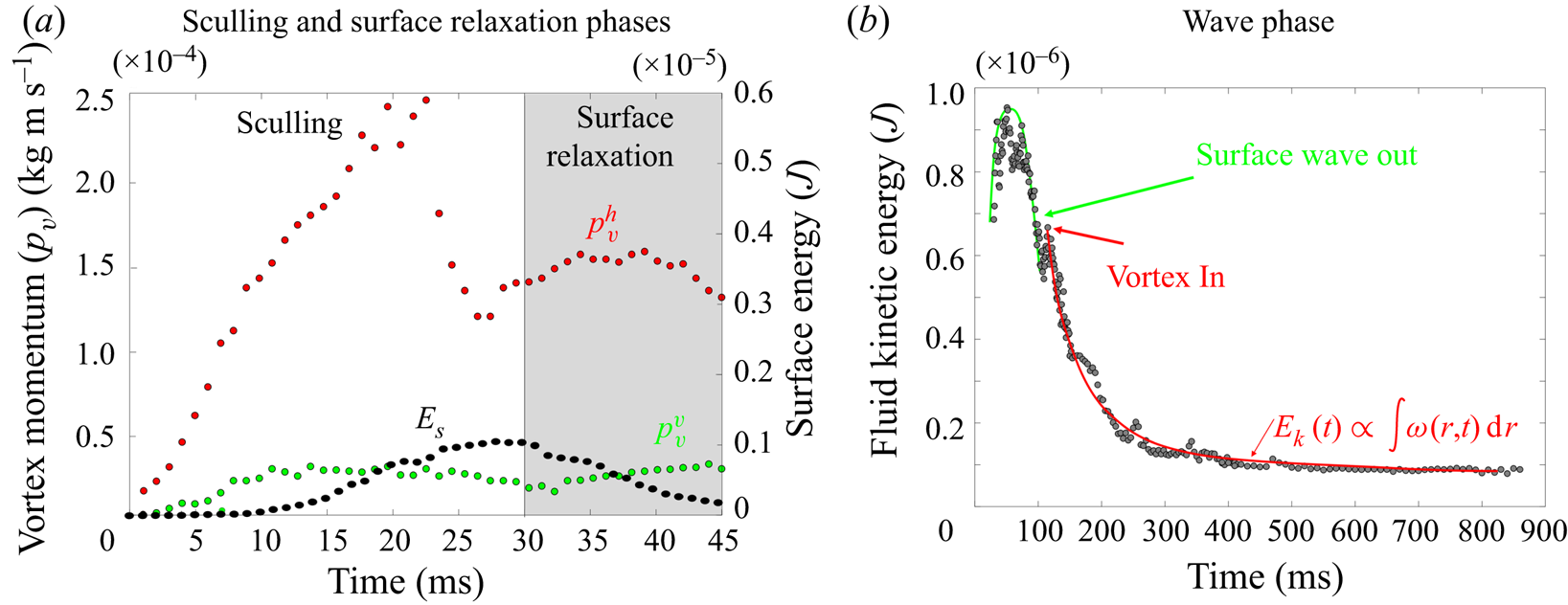
Figure 10. (a) Change in horizontal  $p_v^{h}$ (red points) and vertical
  $p_v^{v}$ (green points) momentum of the vortex, and interface energy
  $E_s$ (black points). These estimated values are derived from the TomoPIV data presented in panels (a,b) of figure 8. (b) Dynamics of kinetic energy in the bulk fluid wake after the propulsion of the water strider. This kinetic energy in the wake is integrated into the measurement volume. These estimated values are derived from the TomoPIV data presented in panels (a,b) of figure 9.
The semi annular vortex is a 3-D structure. To evaluate its force and geometrical change through time, we analyse the evolution of its momentum estimated from two different planar sections: a horizontal section, at the surface of water, and a vertical section crossing the middle of the tarsi and perpendicular to the tarsi extent. We used the procedure of Drucker & Lauder (Reference Drucker and Lauder1999) to characterize this semi annular vortex. The momentum  $p_v(t)$ (kg m s
 $^{-1}$) of a semi-vortex ring shed into the wake is estimated from planar sections using (Petit, Hulin & Guyon Reference Petit, Hulin and Guyon2012)
 \begin{equation} p_v(t)=\tfrac{1}{2}\rho \varGamma_v(t) {\rm \pi}R^{2}, \end{equation}
where  $\rho$ (
 $\textrm {kg}\ \textrm {m}^{-3}$) is the water density,
  $R (m)$ the radius of the vortex ring and
  $\varGamma _v$ (
 $\textrm {m}^{2}\ \textrm {s}^{-1}$) the circulation. The circulation, which measures the strength of the semi-annular vortex, is computed using (2.4). Equation (2.5) expressed the estimation of the momentum of the vortex in two dimensions, obtained from 2-D planar PIV or 2-D numerical simulations in a vertical cross-section of the flow. The vortex momentum, expressed by (3.1) is integrated this time over its volume with dimensionality of momentum (leading to kg m s
 $^{-1}$).
We have estimated the total circulation  $\varGamma ^{h}_v(t)$ at the interface by averaging the absolute circulation obtained from the analysis of two horizontal counter-rotating vortices. This allowed us to determine the time evolution of the momentum in the horizontal plane
  $p^{h}_v(t)=\frac {1}{2}\rho \varGamma ^{h}_v(t) {\rm \pi}R_h^{2}, R_h$ being the apparent vortex ring radius in the horizontal plane estimated as half the distance between the two counter-vortex cores (
 $R_h = 6$ mm). An example of the surface of integration for the calculation of horizontal circulation
  $\varGamma ^{h}_v(t)$ and momentum in the horizontal plane
  $p^{h}_v(t)$ is visible in figure 8(a.iii) for
  $t=20$ ms and figure 8(b.iii) for
  $t=35$ ms. In that figure, the red surface represents the surface of asymptotic circulation. The temporal evolution of the momentum in the horizontal plane is represented by the red circle in figure 10a. We have then estimated the total circulation
  $\varGamma ^{v}_v(t)$ in the vertical plane
  $(x,z)$, crossing the middle of the surface-leg contact line, by integrating the vorticity in an increasing surface until an asymptotic value was attained (Willert & Gharib Reference Willert and Gharib1991). This allowed us to determine the time evolution of the momentum in the vertical plane
  $p_v^{v}$. The surface of integration for the calculation of both the vertical circulation
  $\varGamma ^{v}_v(t)$ and the momentum in the vertical plane
  $p^{v}_v(t)=\frac {1}{2}\rho \varGamma ^{v}_v(t) {\rm \pi}R_v^{2}$ is shown in green in figure 8(a.ii) for
  $t=20$ ms and in figure 8(b.ii) for
  $t=35$ ms. We have estimated
  $R_v$, the apparent vortex ring radius in the vertical plane, as the distance between the leg and the vortex core (
 $R_v = 3$ mm), for the vertical momentum calculation. We represent these momenta and compare them to the energy of the surface over time in figure 10(a).
We estimated the energy in the wake by integrating the kinetic energy in the measurement volume,  $E_k(t)=\int _V {\boldsymbol u}^{2}(x,y,z,t)\, {\textrm {d} x}\, {\textrm {d} y}\, \textrm {d}z$ (figure 10b). The maximum of wave energy travels through the volume between 30 and 80 ms. There is a peak of energy of the flow field during the passing of the wave around 50 ms,
  $E_{kmax}=0.95\times 10^{-6}$ J. We evaluate the gravity–capillary waves velocity to 34 cm s
 $^{-1}$. The waves then leave the measurement volume around 80 ms. A large decrease of energy is observed between 80 and 100 ms. Around 100 ms, a rebound of energy is observed, corresponding to the time at which the vortex enters the measurement volume. This semi-annular vortex travels through the measurement volume (figure 9b) with a convection velocity of
  $V_{vortex} =2.8$ cm s
 $^{-1}$. The energy of the vortex decreases as the integral of vorticity distribution
 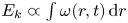 $E_k\varpropto \int \omega (r,t)\, {\textrm {d}}r$, following Lamb–Oseen vortex theory (Saffman Reference Saffman1970; Tinaikar, Advaith & Basu Reference Tinaikar, Advaith and Basu2018). The vorticity distribution is:
  $\omega (r,t)=({\varGamma _0}/{4{\rm \pi} \nu t})\ \textrm {e}^{-(r^{2}/4\nu t)}$. Here,
  $\varGamma _0$ stands for initial circulation while
  $\omega , \nu , r$ and
  $t$ represent the vorticity distribution, kinematic viscosity of the fluid, radial distance from the core centre and time, respectively. So, in the wake, at larger spatial and temporal scales, the vortex was found to travel at a much lower convection speed than the gravity–capillary waves. We also found that the waves transport more kinetic energy than the vortex and that the correct estimation of the energy transported by the vortex depends greatly on the timing of estimation, due to fast dissipation (figure 10b).
For further quantification of all the forces acting on a leg – viscous, pressure and capillary forces – we combined these results with highly reproducible experiments using a mechanical leg model and numerical simulations. Indeed, water striders are small and fast, and their jerky movements are highly variable, making it very difficult to obtain precise measurements at a small scale.
3.2. Mechanical experiments and numerical simulations of the sculling phase
We present here the results of the simulation of the water strider leg physically with a cylinder of steel identical in diameter and length to the leg of the animal ( $D=0.1$ mm,
  $L=40$ mm). It was curved to mimic the deformed shape of the tarsi (figure 7). We simplified the kinematics of the leg by focusing on early time points in the propulsion phase and the almost vertical 1-D displacements of the leg (figure 7). This made it possible to assess the importance of leg speed and depth independently. Water displacement was quantified by 2-D PIV. We also present several computational simulations of interfacial flow in identical situations, using finite-element simulations of the coupled equations describing interface position and flow field.
3.2.1. Dynamics of the interface topography and bulk flow
Our time-resolved 2-D PIV measurements on a mechanical leg allow us to determine the dynamics of the air–water interface topography, as presented respectively in figure 11, for experiments on mechanical leg and numerical simulations. When starting a stroke, the meniscus is symmetrical. As velocity increases, the process of momentum transfer appears. In figure 11, we notice the growing asymmetry of the meniscus, reflecting an increase of the water surface resistance. The posterior and anterior angles  $\alpha _p$ and
  $\alpha _a$ of the dimple deformation are similar in both experiments and model. The progressive increase of the bow wave and its shape are also similar. For both experiments and simulations, the surface breaks at the same time (
 $t=30$ ms). It is visible in the lower panels of figure 11, as the section of mechanical leg and cylinder in the numerical simulations have both crossed the interface. This comparison of the numerical simulations with mechanical experiments showed that the computations were quite realistic, even for key details, such as the temporal changes in dimple morphology, or the magnitudes of the bow wave momentum.
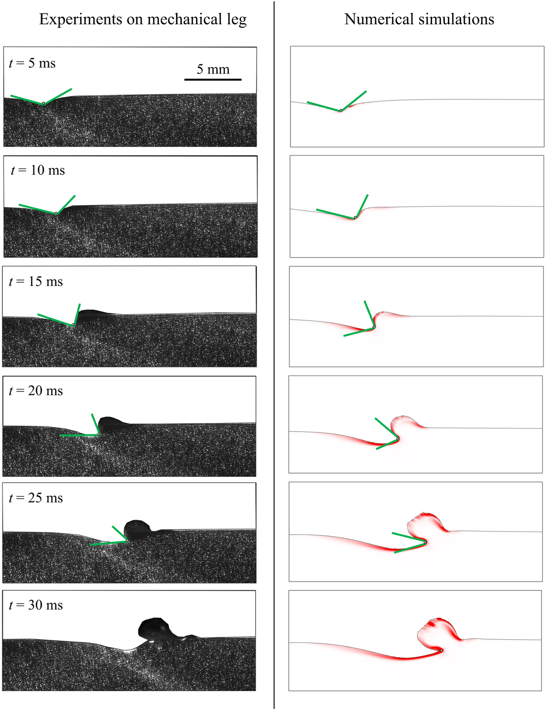
Figure 11. Mechanical and numerical simulations of the transverse motion of a model leg. Comparison between experiments and numerical simulations of the dynamics of the interface and underlying flow;  $h_l=0.95$ mm and
  $V_l=67$ cm s
 $^{-1}$. The leg diameter was 100
  $\mathrm {\mu }$m in the experiments and was 200
  $\mathrm {\mu }$m in the simulations.
3.2.2. Influence of leg velocity and depth of stroke on momentum partitioning
For both mechanical experiments and numerical simulations, we derived the bow wave momentum, the vortex momentum and the capillary forces. We have first studied both experimentally and numerically the effect of variations of propulsion speed at constant depth ( $h_l = 0.95$ mm). We conducted the comparison at this depth as it is the only one for which the surface integrity is maintained, whatever the speed of propulsion. The flow in a vertical cross-section under the surface deformed by a moving mechanical leg and the corresponding numerical simulations are presented in figure 12(a). At constant depth, when the leg velocity increases, we observe that the asymmetry of the interface increases. This results in an increase of the surface tension force and the momentum of the vortex increases up to a certain speed. Its intensity then decreases at higher leg velocity. The volume of the bow wave increases with the leg velocity, which increases its momentum. At high speed, this bow wave is very large. A more detailed view of these results as well as the numerical values are available in figure S2 of the supplementary material and movies are available at https://doi.org/10.1017/jfm.2021.156.
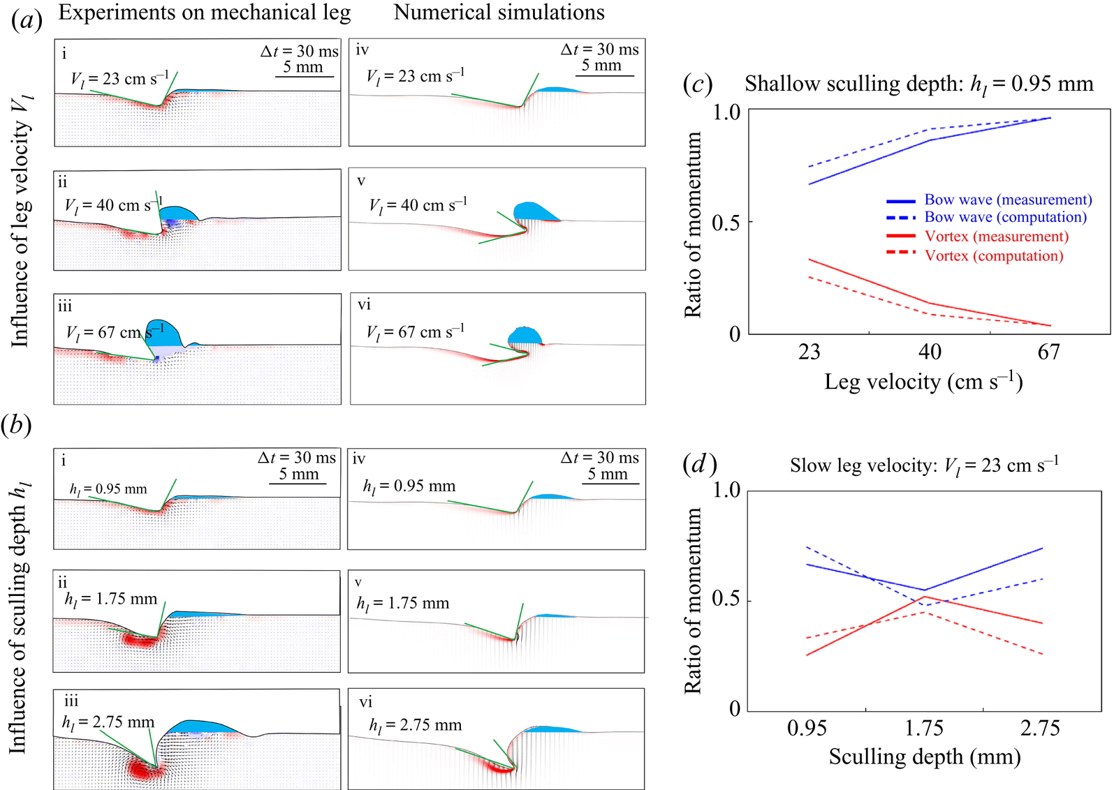
Figure 12. Comparison between experiments and numerical simulations of a sculling leg at the air–water interface. For each measurement and simulation in (a) and (b), the estimation and comparison are done at  ${\rm \Delta} t=30$ ms after the start of the translation. (a) Influence of the velocity of stroke
  $V_l$ on forces and momentum contributions at fixed depth
  $h_l=0.95$ mm. (b) Influence of depth of stroke on forces and momentum contributions at fixed velocity
  $V_l=23$ cm s
 $^{-1}$. (c) Changes in momentum transfer ratios between the bow wave and vortex as a function of sculling depth, for numerical computations and mechanical experiments. (d) Changes in momentum transfer ratios between the bow wave and vortex as a function of leg velocity, for numerical computations and mechanical experiments. Numerical values are available in SI figures S2 and S3.
We have then explored the effect of variations of propulsion depth at constant speed ( $V_l= 23$ cm s
 $^{-1}$). We conducted the comparison at this velocity as it is the only one for which the surface integrity is maintained, whatever the depth of propulsion. Figure 12(b) represents the flow, in a vertical section, under the deformed surface produced by a moving mechanical leg and the corresponding numerical simulations. As the depth increases, we notice that the asymmetry of the interface increases, which increases the surface tension force, and the momentum of the vortex in the flow increases. Furthermore, the volume of the bow wave increases, which increases its momentum. A more detailed view of these results as well as the numerical values are available in figure S3 of the supplementary information.
The range of leg velocities and depths observed for striders is large, so we explored velocities from 20 to 72 cm s $^{-1}$ and depths from 600
  $\mathrm {\mu }$m to 3 mm (the matrix of experiments in the velocity-depth parameter space is visible in figure 5). For both mechanical and computational simulations, momentum transfer to the bow wave is usually higher than that to the vortex (figures 12c and 12d). This resolves the vexing issue of momentum partitioning raised in all previous studies: momentum is mostly transferred in the bow waves rather than in vortices.
3.2.3. Estimation of forces
Our numerical simulations were validated by experiments carried out with a mechanical leg. From these numerical simulations, we deduced the relative importance of the three forces acting on the legs during their displacement on the surface of the water. Two examples of the numerical values of the estimated forces and their respective temporal evolutions are available in figure 13. This figure, illustrating the temporal evolution of the forces, is produced according to two numerical simulations for two couples of velocity (23 and 67 cm s $^{-1}$) and depth (0.95 and 2.75 mm). To cover the full range of conditions we have proceeded to 25 simulations for 25 couples of velocity (10, 18, 23, 30, 40 cm s
 $^{-1}$) and depth (0.1, 0.3, 0.95, 1.75, 2.75 mm). We determined the relative contributions of the drag forces (the sum of viscous (
 $\boldsymbol {F_v}$) and pressure (
 $\boldsymbol {F_p}$) forces) and the capillary force
  $\boldsymbol {F_s}$. We estimated that the viscous drag force is negligible and that the interface resistance force dominates the pressure drag force at almost all regimes of propulsion. Even though water striders have a large plasticity of locomotion involving the use of different mechanisms of force transfer acting on a leg, the capillary force is by far the most important (figure 14a). Striders can, however, benefit from the resistance of the interface, even if they move their legs at a speed below the capillary speed (figure 14a).
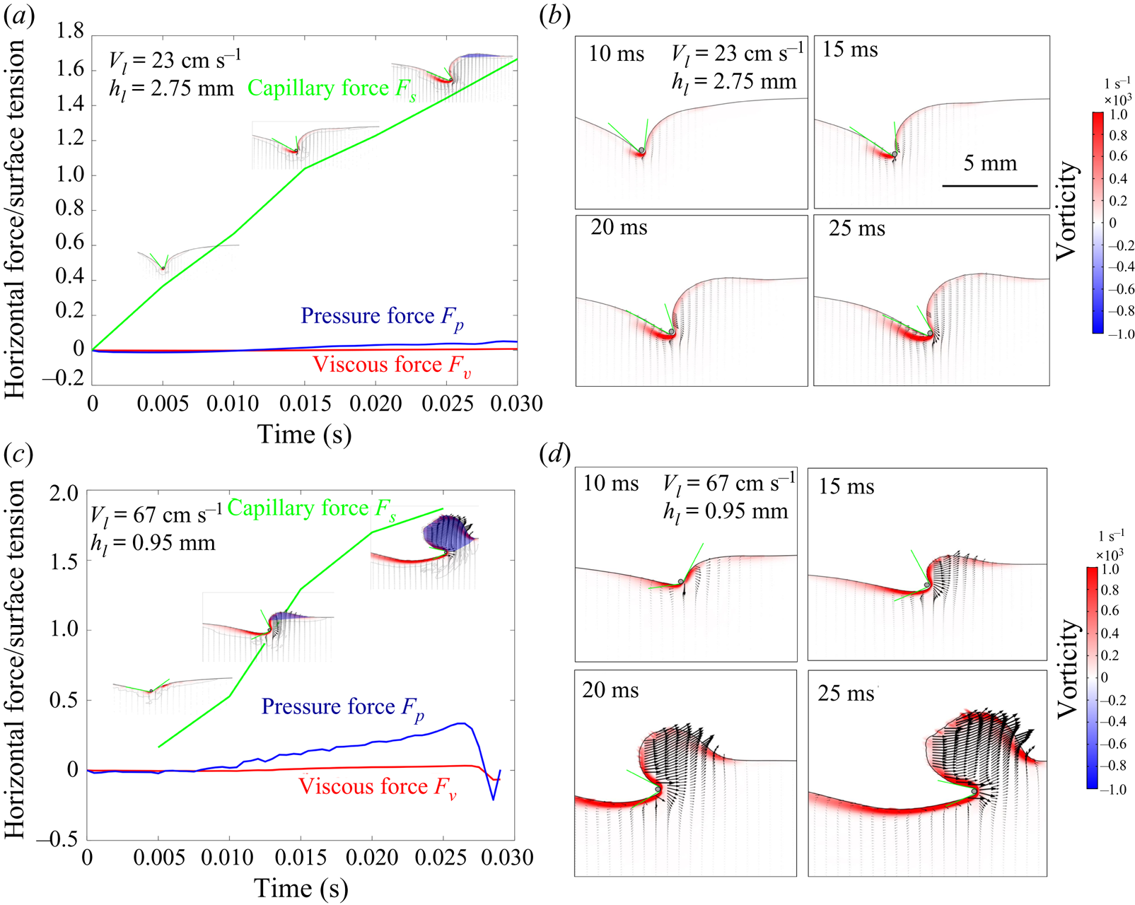
Figure 13. Temporal evolution of the viscous ( $\boldsymbol {F_v}$), pressure (
 $\boldsymbol {F_p}$) and capillary (
 $\boldsymbol {F_s}$) forces produced according to the computation of two numerical simulations. (a) Temporal evolution of the three forces for a leg sculling at
  $V_l=23$ cm s
 $^{-1}$ and
  $h_l=2.75$ mm. (b) Temporal evolution of the air–water interface and vorticity in the water for a leg sculling at
  $V_l=23$ cm s
 $^{-1}$ and
  $h_l=2.75$ mm. (c) Temporal evolution of the three forces for a leg sculling at
  $V_l=67$ cm s
 $^{-1}$ and
  $h_l=0.95$ mm. (d) Temporal evolution of the air–water interface and vorticity in the water for a leg sculling at
  $V_l=67$ cm s
 $^{-1}$ and
  $h_l=0.95$ mm.
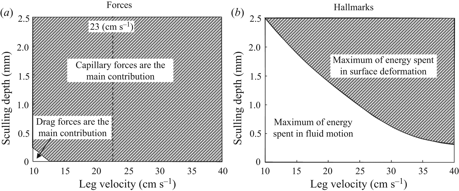
Figure 14. Analysis of forces and hallmarks for numerical simulations of the transverse motion of a model leg. Panels (a,b) were generated from an analysis of the results of numerical simulations of the interface and fluid for sculling legs. We performed 25 simulations for 25 combinations of velocity (10, 18, 23, 30, 40 cm s $^{-1}$) and depth (0.1, 0.3, 0.95, 1.75, 2.75 mm). The dividing lines in (a) and (b) indicate an equal balance between the forces and energy spent, respectively. (a) Relative contributions of the drag forces (the sum of viscous (
 $\boldsymbol {F_v}$) and pressure (
 $\boldsymbol {F_p}$) forces) and the capillary force
  $\boldsymbol {F_s}$. We show the ratio of forces in the space delimited by the depth of sculling and leg velocity. We indicate by a vertical dotted line the minimal gravity–capillary wave velocity of 23 cm s
 $^{-1}$. (b) Ratio of the energy used to deform the surface to the energy used to move the fluid. This figure is based on an analysis of potential, curvature and kinetic energies (at
  $t=15$ ms).
3.2.4. Energy transfer in surface and bulk flow during propulsion
We have also used an alternative approach to a partitioning of momentum, based on energy analysis. We have estimated the surface deformation (potential and curvature) energies together with the water kinetic energy, from our numerical simulations of sculling legs at various depths and velocities. We compared the respective magnitudes of surface and fluid energies for different sculling regimes, delimiting two regions in the depth/velocity space (figure 14b): an upper region where a maximum of energy is spent to deform the interface and a lower region where a maximum of energy is used to put the fluid in motion. Thus, the maximal percentage of energy spent in the water surface deformation or in the fluid bulk depends on the speed of the animal and the depth of leg pulling.
4. Discussion
4.1. Limitations of our experiments and simulations
The combined estimation of the interface topography and the 3-D velocity field below the interface is especially challenging (Chatellier et al. Reference Chatellier, Jarny, Gibouin and David2013; Gomit et al. Reference Gomit, Chatellier, Calluaud and David2013). The choices we made, concerning laser illumination direction, camera position and water tank geometry, have consequences. For instance, the side illumination of a wavy air–water interface often results in the appearance of shadow patches at the surface, due to wave crests. Here, these shadow patches sometimes prevented the identification of the particles at the interface. We proposed and developed very recently an advanced method (Steinmann et al. Reference Steinmann, Casas, Braud and David2021) which circumvents some of these limitations, but this technique requires testing on simpler set-ups, before being applied to more complex ones with living organisms.
The experimental results on the 3-D kinematics of a natural leg (figure 7) have shown that during the first 20 ms of a propulsion step, the leg is largely parallel to the interface and makes a horizontal dimple of at least 1 cm, as previously determined by several authors (Suter et al. Reference Suter, Rosenberg, Loeb, Wildman and Long1997; Suter, Wildman & College Reference Suter, Wildman and College1999; Hu et al. Reference Hu, Chan and Bush2003). This dimple is much higher than the capillary length  $l_c=2.7$ mm. Given that aspect ratio, we expected to encounter a negligible 3-D end effect and decided to treat the problem as two-dimensional, as long as we measure at the centre of the leg. Following Gao & Feng (Reference Gao and Feng2010), we simplified the problem by modelling the leg as a 2-D solid cylinder, without taking into account the complex microstructures of the leg surface. These authors have already justified the relevance of such an approach to the 3-D reality. We notice, however, some small differences between the numerical and mechanical simulation results. The vortex force, notably, is slightly larger in experiments than in computations. These minor differences in magnitude could be partly explained by the 2-D approximation. Only a complete and computationally costly 3-D numerical simulation would allow us to achieve a better fit between experiments and numerical simulations.
A more important difference is that the leg diameter was set to 200  $\mathrm {\mu }$m in our numerical simulations. It is thus twice as large as the diameter of the mechanical legs used in our experiments (100
  $\mathrm {\mu }$m). We preferred to simulate larger legs because, as explained by Gao & Feng (Reference Gao and Feng2010), computing thinner ones becomes computationally very costly, as it would require a thinner diffuse interface to approach the sharp interface limit. This difference in diameters could explain the small divergences observed between mechanical leg experiments and numerical simulation results. Fortunately, as we explain in the following discussion, the complete mechanisms of bow wave and vortex generations could be tackled by considering exclusively the movement of the meniscus, whose shape and volume are very similar for legs of diameter between 100 and 200
  $\mathrm {\mu }$m. For such small leg diameters, the static and dynamic meniscus shapes depend indeed very little on the diameters of the leg and rather on the initial depth and leg velocity (de Gennes, Brochard-Wyart & Quere Reference de Gennes, Brochard-Wyart and Quere2004). We can, however, using larger diameter in our simulations, expect greater differences in the forces exerted by the fluid on the leg, as these are integrated on the leg surface. So, we consider that we slightly overestimated the pressure and viscous forces in the following discussion on the relative magnitude of different forces exerted on the leg.
In the numerical simulation, we did set the initial conditions of the equilibrium interface as determined by the force balance between interfacial tension and hydrostatic pressure by slowly moving down the wetted cylinder to the nominal depth of stroke  $h_d$, as defined in the mechanical simulations. It then formed a symmetric dimple, whose lateral extent is characterized by the capillary length
  $l_c$ (figure 6). Gao & Feng (Reference Gao and Feng2010) rather choose to set their initial conditions by geometrically defining the meniscus profile using the analytical solution of de Gennes et al. (Reference de Gennes, Brochard-Wyart and Quere2004). We show in figure S4 that both our experimental and numerical simulations of the initial interface deformation are very similar to the meniscus profile obtained using that analytical solution.
4.2. Sculling produces a single semi-annular vortex
Hu et al. (Reference Hu, Chan and Bush2003) showed that water striders produce not only waves, but also and mainly a semi-annular vortex, whose momentum is close to that of the insect. The simulations of Gao & Feng (Reference Gao and Feng2010) also show the existence of a vortex, which they claim to be of a different nature from that described by Hu et al. (Reference Hu, Chan and Bush2003). We have, however, shown that the vortices highlighted by Hu et al. (Reference Hu, Chan and Bush2003) and Gao & Feng (Reference Gao and Feng2010) are actually the same and only one. It was merely observed from different point of views. We show that, during the propulsion, the vortex as observed from above in the horizontal plane and as observed from the side in the vertical plane constitutes a single half-ring vortex. In addition, we have estimated that the circulation in both the horizontal and vertical planes are equivalent, especially after the relaxation of the interface. However, the estimation of the momentum of the vortex is greatly affected by the correct estimation of its geometry, as its momentum is not only proportional to its circulation but also to its radius ((3.1)). So, a horizontal, 2-D estimation greatly overvalues the size of the semi-annular vortex ring due to the spacing between the two vortex centres. In its horizontal plane, the vortex radius was  $R_h= 6$ mm, while its radius was
  $R_v= 3$ mm in its vertical plane. Therefore, a horizontal point of view increases de facto the vortex force and its capacity to transport momentum. From the horizontal point of view we estimated a maximal momentum of
 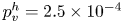 $p_v^{h}=2.5\times 10^{-4}$ kg.m s
 $^{-1}$, whereas the vertical one estimated a maximal momentum of
 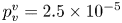 $p_v^{v}=2.5\times 10^{-5}$ kg.m s
 $^{-1}$, a difference of an order of magnitude. It is only by taking the vortex 3-D geometry into account that a faithful estimate of its momentum is obtained.
Our results on living animals reconcile the conflicting views described earlier concerning the number (only one), geometry (half a donut, of diameter varying according to depth) and momentum content of vortices, constituting a first step towards a balance of momentum and energy transfer. They furthermore highlight the importance of both the timing at which a balance is estimated and the size of the control volume. Early instants might miss the full onset of the vortex while later instants miss the rapidly diverging surface waves and need to correct for fast dissipation and energy transfer between surface and vortex. A small control volume misses some of the surface waves too but identifies the exact contours of the vortex while a large control volume cannot sufficiently discern details.
4.3. Vortex regains from surface relaxation
During the sculling phase, TomoPIV measurements (figure 8a) revealed the immediate generation of a single semi-annular vortex (figures 8a.i, 8a.ii and 8a.iii). The geometry of this vortex closely follows the geometry and displacement of the dimple, with marked flattening in the horizontal plane (figure 8a.i). The interface relaxes and becomes horizontal again when the leg detaches from the water surface (figure 8b). The momentum analysis (figure 10a) shows a decrease of the water surface energy when the leg leaves the water surface, at 30 ms. The horizontal momentum of the vortex first stabilizes and then decreases due to viscous damping. At the same time, the vertical momentum of the vortex, which had already decreased, increases again. So the rotation of the flow is enhanced in the vertical plane, after the leg has left the interface and despite a lack of momentum transfer. We have seen that a substantial amount of the energy stored (or carried) in the deformed interface radiates by generating a wave (figure 10b). We have also shown that during the surface relaxation, the large vertical velocity of the depressed interface is sufficient to pull the fluid up, as emphasized in figure 8(b.ii). The transfer of energy between the surface and the fluid leads to a doubling of the vertical momentum of the vortex, from  $1.5\times 10^{-5}$ to
  $3.0\times 10^{-5}$ kg.m s
 $^{-1}$ (figure 10a). These increases in vorticity occur in the absence of momentum transfer, as the insect's leg has already left the surface. They must, therefore, result from surface relaxation. We therefore conclude that the relaxation of the surface contributes greatly to the increase of the observed vorticity in the vertical plane of the semi annular vortex, implying a geometrical reconforming of the semi annular vortex.
There is a striking similarity between these air–water interface deformations occurring during the sculling phase and the cavity observed after a drop impact on an interface (Rein Reference Rein1993, Reference Rein1996; Leng Reference Leng2002; Agbaglah et al. Reference Agbaglah, Thoraval, Thoroddsen, Zhang, Fezzaa and Deegan2015; Thoraval, Li & Thoroddsen Reference Thoraval, Li and Thoroddsen2016; Michon, Josserand & Séon Reference Michon, Josserand and Séon2017; Steinmann et al. Reference Steinmann, Casas, Braud and David2021). Zhang et al. (Reference Zhang, Liu, Qu and Hu2019) also proposed and experimentally observed a phenomenon of energy conversion, between surface potential/curvature energies and fluid kinetic energy, during the retractation of the cavity produced after the impact of a droplet on an interface. We therefore suppose that once the leg has left the air–water interface, the deformed surface energy is transferred to the fluid and converted into kinetic energy. It is an unexpected phenomenon, and has never been observed in animal locomotion. It also indicates that mapping between the forces imparted and hallmarks is not straightforward.
4.4. The main propulsive force is the surface tension and there is no one-to-one mapping between forces and hallmarks
Our numerical simulations were validated by experiments carried out with a mechanical leg. From these numerical simulations, we deduced the relative importance of the three forces acting on the legs during their displacement on the surface of the water. We estimated that the viscous drag force is negligible and that the capillary force dominates the pressure drag force at almost all regimes of propulsion. We thus validated the hypothesis and the results of Gao & Feng (Reference Gao and Feng2010) by showing that the surface tension force is predominant in most cases. Dominance of capillary force (for this leg diameter, very small compared to the capillary length) was also stated by Hu & Bush (Reference Hu and Bush2010). But none of these studies provide physical measurement of capillary forces. Figure 14(a) also shows that the insect can benefit from the resistance of the interface even if it moves its legs at a speed lower than the capillary speed, without the emission of gravity–capillary waves. Thus, the fact that we do not see surface waves then does not mean that there was no transfer of forces between the interface and the leg. At low velocity ( $V_l< 23$ cm s
 $^{-1}$), the main propulsive force is still the interface resistance, but the transfer of momentum results mainly in the appearance of a vortex. This highlights the lack of mapping between forces and hallmarks, with the consequence that the estimation of the momentum imparted in waves and vortices does not give much insight on the main propulsive force. We also confirmed that both hallmarks of momentum transfer could be observed during locomotion. An overlay of forces (figure 14a) and hallmarks (figure 14b) shows an absence of one-to-one mapping, as the propulsion regimes (depth/velocity) in which drag forces predominated does not match the regimes in which a maximum of energy is spent in fluid motion (figures 14a and 14b). The analogy between flying, swimming and moving at the interface collapses here, due to the lack of one-to-one mapping between forces and hallmarks. As a consequence, the main propulsive forces cannot be estimated by measuring momentum and energy partitioning in the fluid and the water strider locomotion has to be treated outside the current framework for animal locomotion. A complete momentum and energy balance is left for the future, as it requires the simultaneous 3-D visualization of both a small control volume around the leg and a large control volume, implying an extremely complex set-up with at least twice as many cameras as used here. Beyond our comprehension of the water strider locomotion mechanism, the precise characterization of the 3-D wake vortex dynamics was also recently defined as a key towards a deeper understanding of animal propulsive efficiency (Dabiri Reference Dabiri2019). Usually, when studying the propulsion of animals and their wakes, we expect that an increase of the vortical wake momentum originates in an increase of pressure drag forces. Using the numerical simulations results, we have estimated how the magnitude of the vortex evolved with an increase of the pressure drag force acting on the leg. We determined that the vortex circulation was not proportional to the increase of pressure drag forces acting on the leg (inset of figure 15 and figure S5 for residuals). We have next estimated how the magnitude of the vortical wake evolved with the increase of the interface resistance force acting on the leg, as shown in figure 15 (and figure S5 for residuals). The strength of the relationship between vortex circulation and pressure drag forces is much weaker than that with capillary forces. The capillary force therefore appears to be the source of the vortex momentum. There is of course a drag force, occurring during leg movement, but this pressure drag does not act on the leg itself, as we explain in the last section.
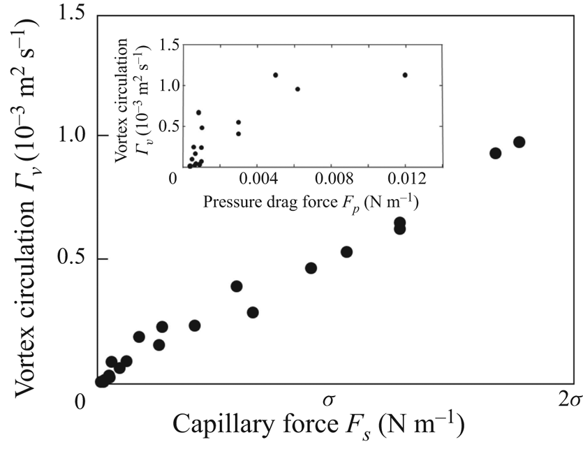
Figure 15. Change in vortex circulation with capillary force acting on the leg contact line. The inset represents the change in vortex circulation with the pressure drag force acting on the leg surface. This figure is based on the analysis of vortex circulation derived from numerical simulations. The data points were obtained from an analysis of the results of numerical simulations of the interface and fluid for sculling legs. We performed 25 simulations for 25 combinations of velocity (10, 18, 23, 30, 40 cm s $^{-1}$) and depth (0.1, 0.3, 0.95, 1.75, 2.75 mm).
4.5. Singularity of the water strider propulsion mechanisms
We are now in a position to describe the full extent and complexity of the mechanics of water strider propulsion. At the start of a leg movement, the fluid is first compressed downstream of the leg. The resulting change in pressure over the water and air is compensated by a large curvature of the surface and the appearance of a bow wave (figure 16). As the fluid flows from the area of high pressure downstream of the leg to the area of low pressure upstream of the leg, a vortex is produced. The decrease in pressure upstream tends to flatten the surface, leading to a dissymmetry of angles at the two contact lines of the leg. A strong horizontal capillary force is then transferred to the leg and the strider moves forward. Thus, the dimple created by the movement of a large amount of water allows the leg to deliver momentum to the fluid through the pressure field, while surface tension maintains its shape and integrity. The pressure field mediating the force transfer acts on the virtual oar made by the leg-plus-dimple, not on the leg. We can show that the pressure drag force rather acts on the dimple, by estimating the magnitude of the pressure force acting on the surface of the moving dimple  $F_p^{dimple}$ and by showing that it is close to the magnitude of the curvature force acting on the leg, as illustrated on figure 16. In this example, the curvature force acting on the leg is
  $F_s=0.127$ N m
 $^{-1}$. This figure also illustrates the pressure field estimated for a leg moving at a depth of
  $h_l=1.75$ mm and at a velocity of
  $V_l=30$ cm s
 $^{-1}$. Indeed, the presence of a zone of large pressure (
 $\boldsymbol {\nabla } p = 60$ Pa) in the 2 mm high bow wave indicates that the pressure force acts essentially on this bow wave. The resulting pressure force (per unit length) can be obtained by multiplying this pressure by the height of the wave to determine that
  $F_p^{dimple}=0.120$ N m
 $^{-1}$.
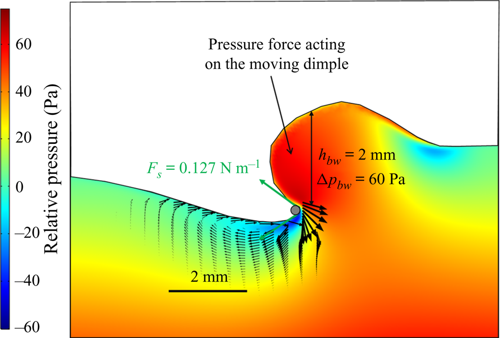
Figure 16. Numerical simulation of the pressure force acting on the moving dimple resulting from the displacement of a leg at a depth of  $h_l=1.75$ mm and a velocity of
  $V_l=30$ cm s
 $^{-1}$. This figure illustrates the equivalence between the magnitude of the capillary force
  $F_s$ acting on the leg and the magnitude of the drag pressure force
  $F_p^{dimple}$ acting on the dimple. The presence of a zone of high pressure (
 $\boldsymbol {\nabla } p = 60$ Pa) in the 2 mm high bow wave indicates that the pressure force acts essentially on this part of the virtual oar, where the bow wave appears. The resulting pressure drag force (per unit length) can be obtained by multiplying this pressure by the height of the wave to obtain
  $F_p^{dimple}=0.120$ N m
 $^{-1}$.
The magnitude of the resulting pressure force is equal to that of the capillary force acting on the leg (figure 16). The virtual oar of the striders is here key, and we observed its size to be up to two orders of magnitude larger than the leg diameter (figure 16).
One remaining question concerns the use of vortices for propulsion. Are they a mere consequence of the interface resistance providing the insect no extra forces? In experiments and numerical simulations, the vortex is situated just below the air–water interface in the upstream part of the leg, a region of low pressure due to its presence (figure 16). The resulting increase of the pressure gradient, between upstream and downstream of the leg, flattens the interface in the upstream part of the leg and contributes to the dissymmetry of the meniscus. The mere presence of the vortex thus enhances propulsion.
Water strider locomotion at the air–water interface is, thus, very effective and different from flying and swimming. In flying animals, drag and lift, the forces resisting wing movement during flight, are integrated over the entire surface of the wing. The wing serves as both the physical interface on which the forces are integrated and the interface pushing the fluid. The same applies to swimming in water, and to any other form of propulsion in which the locomotor organ is totally immersed in the fluid. In striders, the forces act on the large meniscus that pushes the fluid, like an oar blade, rather than the tiny leg (Denny Reference Denny2004). The size of this virtual oar is function of both hydrophobicity-enhancing structural and material properties and leg kinematics. The ability of water striders to gain maximum benefits from water surface deformation may account for the evolution of some of the extravagant morphological innovations observed at the tip of the legs, such as fans (Armisn et al. Reference Armisén, Nagui Refki, Crumiére, Viala, Toubiana and Khila2015; Santos et al. Reference Santos, Le Bouquin, Crumiere and Khila2017). Wing aeroelasticity has been shown to make a major contribution to the optimization of aerodynamics in insects and birds (Zhao et al. Reference Zhao, Huang, Deng and Sane2010; Ramananarivo, Godoy-Diana & Thiria Reference Ramananarivo, Godoy-Diana and Thiria2011; Matloff et al. Reference Matloff, Chang, Feo, Jeffries, Stowers, Thomson and Lentink2020). Tarsal elastocapillarity (Vella Reference Vella2008; Roman & Bico Reference Roman and Bico2010), in addition to super-hydrophobicity (Feng et al. Reference Feng, Gao, Wu, Jiang and Zheng2007; Shi et al. Reference Shi, Niu, Liu, Liu, Wang, Feng and Zhang2007), may be under similarly strong selection pressure in insects living at the water surface.
Supplementary material and movies
Supplementary material and movies are available at https://doi.org/10.1017/jfm.2021.156.
Acknowledgements
We thank Drs M. Pineirua and M. Jaffar-Bandjee for insighful discussions and the reviewers for their comments which did improve the manuscript.
T.S. and J.C. defined the question, A.C. performed the mechanical simulations, T.S. performed the numerical computations and derived the analytical theory. All authors contributed equally to analysing data and reaching conclusions, and in writing the paper.
Funding
The Tomo-PIV equipment was obtained through the CPER-Région Centre grant Biopatic to J.C.
Declaration of interests
The authors report no conflict of interest.