
General Systems Theory faces several challenges in the context of science development. One of them is to provide social and human sciences with an epistemological status similar to that of applied sciences (physics, chemistry, biology, economics, etc.). A way to deal with this challenge is to find validated mathematical dynamic models for magnitudes of social interest with the same predictive potential as the existing models used in applied sciences. In addition, such mathematical models should be expressed using the same universal language as in the applied sciences, i.e., in terms of differential/integral/finite-difference equations, which have proved to be so fruitful and successful in the positive sciences. This approach also permits to compare models and systems, as well as to classify them into categories, independently of their discipline, i.e., to build general systems. With respect to uncertainties, there are mathematical methods adequate to deal with uncertainties, data errors and personal estimations, producing results with its respective confidence intervals.
This article is a first attempt to face this challenge in the context of personality theory. Concretely, we discuss in this paper a dynamic mathematical approach to understand personality from the perspective of a general factor of personality (GFP) and its relationships with the Big Five Factors (B5F). On the one hand, we propose only one mathematical model to describe the dynamic pattern of response of the GFP and the B5F as a consequence of the same stimulant drug single dose. Let this model be named as the response model. In the application case performed in order to validate the response model, the stimulus is caffeine, considered as a stimulant drug. Acute doses of caffeine, at levels typically found in a cup of coffee, produce stimulant-like subjective effects (Childs & de Wit, Reference Childs and de Wit2006; Nehlig, Reference Nehlig1999). On the other hand, assuming that each factor dynamics holds the response model, i.e., under the invariance of its dynamic pattern, the mathematical relation among these factors is obtained. Let this mathematical relation be named as the bridge model. In other words, both the GFP and the B5F co-evolve in time, as a consequence of the same stimulus, with values connected by the bridge model.
The General Factor of Personality and the Big Five Factors
The existence of a GFP is claimed by the Unique Personality Trait Theory (UPTT) (Amigó, Reference Amigó2005), which proposes a hierarchical approach where the highest level corresponds to the unique trait (the GFP), extended from an impulsivity and aggressively pole (approach tendency) to an anxiety and introversion pole (avoidance tendency). Following the UPTT, the brain activation level represents the biological base of the GFP.
There are evidences of the existence of a GFP to describe the overall personality and its relationships with the B5F (Amigó, Reference Amigó2005; Amigó, Caselles, & Micó, Reference Amigó, Caselles and Micó2008; Rushton & Irwing, Reference Rushton and Irwing2008), as well as its biological base (Amigó, Reference Amigó2005; Amigó, Caselles, Micó, & García, Reference Amigó, Caselles, Micó and García2009a; Micó, Amigó, & Caselles, Reference Micó, Amigó and Caselles2012; Rushton, Bons, & Hur, Reference Rushton, Bons and Hur2008).
Actually, the structural model of personality that has attracted the most research interest has been the Big Five model (Digman, Reference Digman1990; McCrae & Costa, Reference McCrae and Costa1987, Reference McCrae and Costa1997). The first proponents of this personality model obtained five robust and orthogonal factors, irreducible basic dimensions. However, there is evidence about these dimensions are strongly related (Becker, Reference Becker1999; Digman, Reference Digman1997; Eysenck, Reference Eysenck1991, Reference Eysenck1992; Wiggins & Trapnell, Reference Wiggins, Trapnell and Wiggins1996).
Several authors found evidence for the existence of a single common factor underlying the Big Five (Figueredo et al, Reference Figueredo, Vásquez, Brumbach, Schneider, Sefcek, Tal and Jacobs2006; Musek, Reference Musek2007; Rushton & Irwing, Reference Rushton and Irwing2008; Rusthon et al., Reference Rushton, Bons and Hur2008; Saucier & Goldberg, Reference Saucier, Goldberg, Barrick and Ryan2003). For example, Musek (Reference Musek2007) confirmed the existence of a GFP (the Big One) characterized by high versus low Emotionality Stability, Conscientiousness, Agreeableness, Extraversion and Openness. He proposed a comprehensive theoretical model of personality structure with the Big One at the highest level of hierarchy. Rusthon et al. (Reference Rushton, Bons and Hur2008) found the same relations pattern among the B5F and the GFP. Some different results were found by Amigó, Caselles, and Micó (Reference Amigó, Caselles and Micó2010), with a GFP positively related with Extraversion and Openness, but negatively related with Neuroticism (what is equivalent to positively related with Emotional Stability), Conscientiousness and Agreeableness.
On the other hand, there is really an only study known by the authors about the interaction between GFP, the B5F and the acute effect of drugs: the one of Corr and Kumari (Reference Corr and Kumari2000). These authors observed some individual differences in the reaction to amphetamine in Psychoticism: d-amphetamine increased the energy arousal and the hedonic tone and reduced the tense arousal in normal individuals whereas the high Psychoticism individuals experienced the opposite pattern. Neither the Search of Newness nor Extraversion modified the effects of d-amphetamine. In addition, no studies about the evolution at very short term (laboratory experiment) of these factors of personality are known by the authors. Thus, an integrating and dynamic model of personality that allows predicting the response of the basic factors of personality (such as the B5F or the GFP) to acute doses of a drug does not exist. The UPTT (Amigó, Reference Amigó2005), offers a theoretical frame to investigate this integration proposal.
The UPTT asserts that the human activation level of the stress system is the responsible of the different responses to a stimulus. Lower tonic activation levels correspond with the impulsivity and aggressively pole (approach tendency), while higher tonic activation levels correspond with the anxiety and introversion pole (avoidance tendency). The activation level response to a stimulus is given by a certain time pattern that can be described mathematically by the response model (Amigó, Caselles, & Micó, Reference Amigó, Caselles and Micó2008; Caselles, Micó, & Amigó, Reference Caselles, Micó and Amigó2010) and explains personality dynamics as a consequence of the effect of a stimulant drug. Thus, the UPTT, which defends the existence of the GFP, is an important theoretical frame to develop a dynamic model of relations between the GFP and the B5F that allows understanding the dynamics of the global personality.
Summarizing, the UPTT and the referred studies present a structural model which is attempted to be represented mathematically here by the response model and by the bridge model. On the one hand, the response model provides the common dynamic pattern for the GFP and the B5F. On the other hand, the bridge model provides the dynamic interrelationship among the GFP and the B5F. Thus, this structural model, given by the pair of both models, has a dynamic nature, showing a co-evolution of all involved factors as a consequence of a same stimulus, rather than an unconnected evolution.
The Mathematical Models
The response model is founded on three basic theories that explain the time pattern of the effects of drugs and the differential reactivity to them, i.e., the opponent-process theory of acquired motivation of Solomon and Corbit (Reference Solomon and Corbit1974), the gated dipole theory of Grossberg (Reference Grossberg2000) and the UPTT of Amigó (Reference Amigó2005). In the study of Amigó et al., (Reference Amigó, Caselles and Micó2008) the GFP dynamics, represented biologically by the brain activation level, is modeled holding the response model from the three basic theories above referred.
In addition, the response model has been used to describe the GFP dynamics under the effect of a single dose of caffeine (Caselles, Micó, & Amigó, Reference Caselles, Micó and Amigó2011). Besides, the response model has also been used to describe the GFP dynamics and the c-fos dynamics (considered as a biological substrate for personality) under the effect of a single dose of methylphenidate (Micó et al., Reference Micó, Amigó and Caselles2012). The substrate of personality has also been studied by the experimental evaluation of the glutamate in blood as a consequence of a single dose of methylphenidate (Amigó et al., Reference Amigó, Caselles, Micó and García2009a; Micó, Caselles, Amigó, Cotolí, & Sanz, Reference Micó, Caselles, Amigó, Cotolí and Sanz2013) and, by the experimental evaluation of the DRD3 gene expression, as a consequence of a suggestion technique (Amigó, Caselles, & Micó, Reference Amigó, Caselles and Micó2013).
On the other hand, the process to obtain the response model is based on the General Modeling Methodology established by Caselles (Reference Caselles1994) within the General Systems Theory context that the same author developed. Caselles (Reference Caselles1992a, Reference Caselles1993, Reference Caselles1995) proposes a modeling process which not only attempts to organize partial methods, but also attempts to include the ideas of Forrester (Reference Forrester1961, Reference Forrester1970), the creator of Systems Dynamics, and the contributions of other authors. The General Modeling Methodology attempts to generalize the scientific method or the hypothetic-deductive method to be applied to model complex systems. Ten stages may be identified in this methodology, and natural feedback processes take place between them instead of them being linearly run.
The response model is constituted by three coupled differential equations, being the state variables the following ones: the non-assimilated drug, the drug in blood (which represents the stimulus), and the GFP. The derivative with respect to time of the GFP is the sum of three flows. Two of them are a consequence of the stimulus while the third flow appears with a finite and positive delay. The first flow, named as homeostatic control, is a mechanism of fast recovering of the tonic GFP. The second flow, named as excitation effect, increases the GFP as a consequence of the stimulus. The third flow is a slow control mechanism, named as inhibitor effect, which after the time delay (named as inhibitor effect delay), decreases the GFP. Thus, the equation corresponding to the GFP is a delay differential equation with finite delay and, therefore, it represents an “all or nothing” phenomenon.
Further simulations show that the model for the effect of a single dose of a stimulant drug can also be described without delay. Nevertheless, an addiction model needs that delay is considered, as Solomon and Corbit point out (1974). The model without delay can reproduce the same dynamic patterns above mentioned. Following the scientific principle of choosing the simplest model, we are going to work, in the context of this paper, with the model without delay, leaving for future research the question of if an addiction model would really need the mathematical consideration of a delay.
Thus, the response model that we propose in this paper is based on the model without delay that describes mathematically the dynamic pattern of both the GFP and the B5F, as a consequence of a stimulant drug intake. According to this assumption, the bridge model is deduced in this paper as a partial differential equation that relates any pair of factors and time. The solutions of the bridge model provide the co-evolution of all factors, as a consequence of a stimulant drug intake.
The Application Case
In order to validate both models, we start from an innovating and little used experimental approach. In this approach, the experimental subjects fill in a list of 25 adjectives that correspond to the B5F (Brody & Ehrlichman, Reference Brody and Ehrlichman1998), requesting to them that they respond so much considering such adjectives as traits (“Are you like that in general? ”) or like states (“Are you like that or feel like that at this moment?”).
Thus, a trait-format and state-format of this list of adjectives exists. This allows us simultaneously to have a version of personality in the trait level and a version of situational personality or in the state level, as much for the B5F as for the GFP. The version of “personality states” allows us to evaluate the personality at every moment and based on the effects of a certain stimulus like caffeine, of a similar manner to the scales of the mood-states or of the effects of situations elaborated specially for this purpose, such as the Multiple Affect Adjective Check List (MAACL, Zuckerman & Lubin, Reference Zuckerman and Lubin1965) or the Profile of Mood States (POMS, McNair & Droppleman, Reference McNair and Droppleman1971). The theoretical foundation of this proposal comes guaranteed by the existing hierarchical models of personality, specially the model of parameters of Pelechano (Reference Pelechano1973, Reference Pelechano2000), that considers three levels of consolidation of the dimensions of personality, from the upper level of consolidation to the situational level or state level. Schutte, Malouff, Segrera, Wolf, and Rodgers (Reference Schutte, Malouff, Segrera, Wolf and Rodgers2003) elaborated a Big Five States Inventory starting from the hierarchical model of personality. Traits are conceptualized as higher-level and enduring characteristics, while states are lower level and less enduring characteristics (p. 592). A factor analysis showed an acceptable fitting between responses on measures of transitory states and the Big Five dimensions. The subjects had to answer: “Describe yourself as you see yourself at the present time not as you wish to be in the future or as you were in the past” (p. 594). They used an experimental manipulation, the positive mood induction procedure, to attempt to change the levels of the Big Five States. There was a significant increase in surgency, agreeableness and openness from pre- to post-induction.
Trait and state can be measured with the considered list of adjectives. This option has two advantages: 1) the isomorphism of the measures, which do not require different instruments for the evaluation of trait and state; 2) the possibility to study the dynamics of personality at short and at long term.
Both, response and bridge models, are validated in the application case, corresponding to an experimental design with twenty adult subjects that consumed coffee with an empty stomach. The instruments of this experiment are: the Big Five Personality Adjectives List (BFPAL) (Brody & Ehrlichman, Reference Brody and Ehrlichman1998) and the Five-Adjective Scale of the General Factor of Personality (GFP-FAS, Amigó, Micó, & Caselles, Reference Amigó, Micó and Caselles2009b).
The validation process has two parts. In the first part, the response model of each factor is fitted to experimental data with the minima squared method. Once the parameter values are obtained (see Tables 1 and 2), the method to assess the response model for each factor is to compute, both for the mean values and for each individual case, the determination coefficients between experimental and predicted data, observing that, in general the coefficients are enough high as to accept the response model (see Table 3). In the second part, considering the parameter values obtained in the first part, the same method is followed to assess the bridge model between pairs of factors, i.e., to evaluate the corresponding determination coefficients (see Table 4). In addition, a visual evaluation of both models is possible through the observation of the figures representing the experimental data together with the predicted data (see Figures 2 to 23), both for the mean data and for Case 1 (considered as one of the most representative cases).
The following sections of the article are organized as follows. Section 2 presents the response model, valid for all factors. In Section 3 the bridge model between each pair of factors and time is deduced from the assumptions set up in Section 2. Section 4 presents the experimental design of the application case. Section 5 presents the response model validation for the six factors (the GFP and the B5F), as well as the bridge model between each pair of factors and time. Section 6 is devoted to the comparison with alternative models and the theory limitations, as well as the separation of the actual results of the paper from the potential use of these results. Section 7 presents the conclusions of the study.
The Response Model
Following the hypothetico-deductive method, we start from a theoretical model that can explain the evolution of the GFP as a consequence of a stimulus and try to validate it through its contrast with real data. Amigó et al. (Reference Amigó, Caselles and Micó2008) presented a model that has enough the theoretical foundation to be worthy of being tested through an experiment with human subjects. Contributing to such validation is the work of Caselles et al. (Reference Caselles, Micó and Amigó2011). In order to make the paper self-contained, let us synthesize this model in this section as well as a modification of the same model (Micó, Amigó, & Caselles, Reference Micó, Amigó and Caselles2008).
Let y(t), b and y 0 be respectively the GFP, its tonic level and its initial value. Amigó et al. (Reference Amigó, Caselles and Micó2008) demonstrate that the delay differential equation that explains the evolution of the GFP as a consequence of a drug intake is:
 $$\eqalign{ & {{dy\left( t \right)} \over {dt}}
= \left\{ {\matrix{ {a\left( {b - y\left( t \right)} \right)
+ {p \over b}s\left( t \right):0 \le t \le \tau } \cr
{a\left( {b - y\left( t \right)} \right) + {p \over b}s\left(
t \right) - b \cdot q \cdot s\left( {t - \tau } \right) \cdot y\left( {t
- \tau } \right):t > \tau } \cr } } \right. \cr
& y\left( 0 \right) = y_0 \cr}$$
$$\eqalign{ & {{dy\left( t \right)} \over {dt}}
= \left\{ {\matrix{ {a\left( {b - y\left( t \right)} \right)
+ {p \over b}s\left( t \right):0 \le t \le \tau } \cr
{a\left( {b - y\left( t \right)} \right) + {p \over b}s\left(
t \right) - b \cdot q \cdot s\left( {t - \tau } \right) \cdot y\left( {t
- \tau } \right):t > \tau } \cr } } \right. \cr
& y\left( 0 \right) = y_0 \cr}$$
Where,
t is time, a, p, q and τ are parameters to be explained later;
s(t), represents the stimulus, i.e., the amount in blood of drug non consumed by cells;
a(b-y(t)) is the homeostatic control, i.e., the cause of the fast recovering of the tonic level b, being a the “power” of this control;
p·s(t)/b is the excitation effect, which tends to increase the GFP, being p the excitation effect power;
b·q·s(t-τ)·y(t-τ) is the inhibitor effect, which tends to decrease the GFP and is the cause of the its slow recovering, being q the inhibitor effect power and being τ the inhibitor effect delay time after which the inhibitor effect takes place (which means that an “all or nothing” effect occurs, similar to the electrochemical transmission in the neuron axon).
Being c(t) the non-assimilated drug, i.e., the drug not yet in blood,
s(t) and c(t) are computed by two coupled differential equations:
 $$\left. {\matrix{ {{{dc\left( t \right)} \over {dt}} =
- {\rm{\alpha }} \cdot c\left( t \right)} \cr {c\left( 0 \right)
= M} \cr } } \right\}$$
$$\left. {\matrix{ {{{dc\left( t \right)} \over {dt}} =
- {\rm{\alpha }} \cdot c\left( t \right)} \cr {c\left( 0 \right)
= M} \cr } } \right\}$$
 $$\left. {\matrix{ {{{ds\left( t \right)} \over {dt}} =
\alpha \cdot c\left( t \right) - \beta \cdot s\left( t \right)} \cr
{c\left( 0 \right) = s_0 } \cr } } \right\}$$
$$\left. {\matrix{ {{{ds\left( t \right)} \over {dt}} =
\alpha \cdot c\left( t \right) - \beta \cdot s\left( t \right)} \cr
{c\left( 0 \right) = s_0 } \cr } } \right\}$$
Where,
M is the initial amount of drug of a single dose;
α is the drug assimilation rate;
s 0 is the amount of drug present in blood before the dose intake;
β is the drug distribution rate.
Equations (1), (2) and (3) define a response model. It reproduces the dynamic patterns forecasted by Solomon and Corbit (Reference Solomon and Corbit1974), Grossberg (Reference Grossberg2000) and Amigó (Reference Amigó2005), and it can be considered theoretically validated through the scientific literature about the subject (Amigó et al., Reference Amigó, Caselles and Micó2008).
The equation obtained by eliminating the delay in equation (1) is the following:
 $$\left. {\matrix{ {{{dy\left( t \right)} \over {dt}} =
a\left( {b - y\left( t \right)} \right) + {p \over b}s\left(
t \right) - b \cdot q \cdot s\left( t \right) \cdot {\rm{y}}\left( t
\right)} \cr {y\left( 0 \right) = y_0 } \cr } }
\right\}$$
$$\left. {\matrix{ {{{dy\left( t \right)} \over {dt}} =
a\left( {b - y\left( t \right)} \right) + {p \over b}s\left(
t \right) - b \cdot q \cdot s\left( t \right) \cdot {\rm{y}}\left( t
\right)} \cr {y\left( 0 \right) = y_0 } \cr } }
\right\}$$
The response model on which we are going to found our deductions is the one formed by Equations (2), (3) and (4). This particular response model has been validated by Micó et al., (Reference Micó, Amigó and Caselles2008). The experimental design presented in this paper confirms that validation. A causal diagram of this model can be found in Figure 1 and, the paper of Amigó et al., (Reference Amigó, Caselles and Micó2008) provides a hydrodynamic diagram that can help to better understand the model with delay from a qualitative approach.

Figure 1. Causal diagram of the response model.
The elimination of the delay in (1) to obtain (4) provides the possibility to obtain the bridge model as a partial differential equation without delays. This makes possible to handle analytically the bridge model (see the following section).
The Bridge Model
The aim of this section is to deduce theoretically a bridge model between each pair of the six considered factors (the GFP and the B5F). Each bridge model is constituted by a partial differential equation and a boundary condition. The solution of this pair of equations provides the co-evolution of the considered factors as a consequence of a single dose of a stimulant drug. In other words, given a value of an arbitrary factor i, and a value of the stimulus, s(t), in a certain time instant t, the value of another but different factor j can be deduced. The validation of the hypothetical response and bridge models by its contrast with experimental data would confirm the common dynamics of all factors and their correlated evolution as a consequence of a single dose of a stimulant drug, what represents a progress towards a unified dynamic theory of personality.
Our hypothesis, in order to obtain the bridge model between each one of the B5F and the GFP, is that the dynamic response of each one of the B5F, as a consequence of a single dose of a stimulant drug, is also provided by equation (4), that is:
 $$\left. {\matrix{ {{{dE_i \left( t \right)} \over {dt}}
= A_i \left( {B_i - E_i \left( t \right)} \right)
+ {{P_i } \over {B_i }}s\left( t \right) - B_i \cdot Q_i
\cdot s\left( t \right) \cdot E_i \left( t \right)} \cr {E_i \left( 0
\right) = E_i^{\left( 0 \right)} } \cr } }
\right\}$$
$$\left. {\matrix{ {{{dE_i \left( t \right)} \over {dt}}
= A_i \left( {B_i - E_i \left( t \right)} \right)
+ {{P_i } \over {B_i }}s\left( t \right) - B_i \cdot Q_i
\cdot s\left( t \right) \cdot E_i \left( t \right)} \cr {E_i \left( 0
\right) = E_i^{\left( 0 \right)} } \cr } }
\right\}$$
Where,
1 ≤ i ≤ 5, and each subscript value corresponds to each one of the B5F, in the following sort: E 1 ≡ E (Extraversion), E 2 ≡ R (Responsibility), E 3 ≡ N (Neuroticism), E 4 ≡ O (Openness to Experience), E 5 ≡ A (Agreeableness);
 $E_i^{\left( 0 \right)}$
is the corresponding initial value in t
= 0;
$E_i^{\left( 0 \right)}$
is the corresponding initial value in t
= 0;
A i , B i , P i and Q i , are the parameters equivalent to the corresponding ones in (4);
s(t) is the stimulus function, i.e., is the same than in equation (4), and obtained through equations (2) and (3).
The assumptions (5.i) come from the visual observation of the scores of each factor plotted versus time. See Figures 2 to 7 for the mean values of the group and Figures 8 to 13 for Case 1. Such figures, where the dots represent the experimental data versus time, suggest a same dynamic pattern, common to all factors. The validation of this hypothesis is performed below, in Section 5.1.
The method followed to obtain the bridge model considers that (4) and (5.i) hold, and finds the equations that keep (4) and (5.i) invariant. Let the functions that relate the B5F, (E i ), time, (t), and the GFP, (y), be the following:
 $$E_i = E_i \left( {t,y} \right)$$
From (6.i), deriving with respect to time, equations (7.i) are obtained:
 $${{dE_i } \over {dt}} = {{\partial E_i } \over
{\partial t}} + {{\partial E_i } \over {\partial y}}{{dy}
\over {dt}}$$
$${{dE_i } \over {dt}} = {{\partial E_i } \over
{\partial t}} + {{\partial E_i } \over {\partial y}}{{dy}
\over {dt}}$$
Substituting (4) in (7.i) equations (8.i) are obtained:
 $${{\partial E_i } \over {\partial t}} + {{\partial E_i
} \over {\partial y}}\left[ {a\left( {b - y} \right) + {p
\over b}s\left( t \right) - b \cdot q \cdot s\left( t \right) \cdot y}
\right] = A_i \left( {B_i - E_i } \right) + {{P_i
} \over {B_i }}s\left( t \right) - B_i \cdot Q_i \cdot s\left( t \right)
\cdot E_i$$
$${{\partial E_i } \over {\partial t}} + {{\partial E_i
} \over {\partial y}}\left[ {a\left( {b - y} \right) + {p
\over b}s\left( t \right) - b \cdot q \cdot s\left( t \right) \cdot y}
\right] = A_i \left( {B_i - E_i } \right) + {{P_i
} \over {B_i }}s\left( t \right) - B_i \cdot Q_i \cdot s\left( t \right)
\cdot E_i$$
Equations (8.i) are quasi-linear partial differential equations that, together with the boundary conditions stated below, define the bridge model. Observe that the use of Equation (1) instead of Equation (4) (without delay) would provide a partial differential equation similar to (8.i) but with different delays for dependent variables, E i (t,y), and for the independent variables, t and y. This equation would be impossible to handle analytically such as it is done in this section. However, it is obvious that a more general bridge model that can include the delays and can be analytically handled must be investigated.
Equations (8.i) can be solved through their characteristic equations:
 $${{dt} \over 1} = {{dy} \over {a\left( {b - y} \right)
+ {p \over b}s\left( t \right) - b \cdot q \cdot s\left( t
\right) \cdot y}} = {{dE_i } \over {A_i \left( {B_i - E_i }
\right) + {{P_i } \over {B_i }}s\left( t \right) - B_i \cdot
Q_i \cdot s\left( t \right) \cdot E_i }}$$
$${{dt} \over 1} = {{dy} \over {a\left( {b - y} \right)
+ {p \over b}s\left( t \right) - b \cdot q \cdot s\left( t
\right) \cdot y}} = {{dE_i } \over {A_i \left( {B_i - E_i }
\right) + {{P_i } \over {B_i }}s\left( t \right) - B_i \cdot
Q_i \cdot s\left( t \right) \cdot E_i }}$$
Two independent coupled differential equations can be extracted from (9.i) for each index value i:
 $${{dy} \over {dt}} = a\left( {b - y} \right)
+ {p \over b}s\left( t \right) - b \cdot q \cdot s\left( t
\right) \cdot y$$
$${{dy} \over {dt}} = a\left( {b - y} \right)
+ {p \over b}s\left( t \right) - b \cdot q \cdot s\left( t
\right) \cdot y$$
 $${{dE_i } \over {dt}} = A_i \left( {B_i - E_i }
\right) + {{P_i } \over {B_i }}s\left( t \right) - B_i \cdot
Q_i \cdot s\left( t \right) \cdot E_i$$
$${{dE_i } \over {dt}} = A_i \left( {B_i - E_i }
\right) + {{P_i } \over {B_i }}s\left( t \right) - B_i \cdot
Q_i \cdot s\left( t \right) \cdot E_i$$
Both (10) and (11.i) have the following analytical solutions, depending respectively on arbitrary constants, k 1 and k 2i :
 $$y \cdot \exp \left( {\int\limits_0^t {h\left( x \right)dx} }
\right) - \int\limits_0^t {g\left( x \right) \cdot \exp \left(
{\int\limits_0^x {h\left( z \right)dz} } \right)dx} =
k_1$$
$$y \cdot \exp \left( {\int\limits_0^t {h\left( x \right)dx} }
\right) - \int\limits_0^t {g\left( x \right) \cdot \exp \left(
{\int\limits_0^x {h\left( z \right)dz} } \right)dx} =
k_1$$
 $$E_i \cdot \exp \left( {\int\limits_0^t {H_i \left( x \right)dx}
} \right) - \int\limits_0^t {G_i \left( x \right) \cdot \exp \left(
{\int\limits_0^x {H_i \left( z \right)dz} } \right)dx} =
k_{2i} $$
$$E_i \cdot \exp \left( {\int\limits_0^t {H_i \left( x \right)dx}
} \right) - \int\limits_0^t {G_i \left( x \right) \cdot \exp \left(
{\int\limits_0^x {H_i \left( z \right)dz} } \right)dx} =
k_{2i} $$
Where:
 $$h\left( t \right) = a + b \cdot q \cdot
s\left( t \right)$$
$$h\left( t \right) = a + b \cdot q \cdot
s\left( t \right)$$
 $$g\left( t \right) = a \cdot b + {p \over
b}s\left( t \right)$$
$$g\left( t \right) = a \cdot b + {p \over
b}s\left( t \right)$$
 $$H_i \left( t \right) = A_i + B_i \cdot Q_i
\cdot s\left( t \right)$$
$$H_i \left( t \right) = A_i + B_i \cdot Q_i
\cdot s\left( t \right)$$
 $$G_i \left( t \right) = A_i \cdot B_i +
{{P_i } \over {B_i }}s\left( t \right)$$
$$G_i \left( t \right) = A_i \cdot B_i +
{{P_i } \over {B_i }}s\left( t \right)$$
Thus, the solutions of (8.i) are given, formally, by:
 $$k_{2i} = \Phi _i \left( {k_i } \right)$$
that is:
 $$\displaylines{ E_i \cdot exp\left( {\int_0^t {H_i \left( x
\right)dx} } \right) - \int_0^t {G_i \left( x \right) \cdot exp\left(
{\int_0^x {H_i \left( z \right)dz} } \right)dx} = \cr \Phi _i
\left( {y \cdot exp\left( {\int_0^t {h\left( x \right)dx} } \right) -
\int_0^t {g\left( x \right) \cdot exp\left( {\int_0^x {h\left( z
\right)dz} } \right)dx} } \right) \cr}$$
$$\displaylines{ E_i \cdot exp\left( {\int_0^t {H_i \left( x
\right)dx} } \right) - \int_0^t {G_i \left( x \right) \cdot exp\left(
{\int_0^x {H_i \left( z \right)dz} } \right)dx} = \cr \Phi _i
\left( {y \cdot exp\left( {\int_0^t {h\left( x \right)dx} } \right) -
\int_0^t {g\left( x \right) \cdot exp\left( {\int_0^x {h\left( z
\right)dz} } \right)dx} } \right) \cr}$$
In order to find the Φi functions, a boundary condition for each equation (8.i) is required. They can be obtained from the differential equations (4) and (5.i) in absence of stimulus, that is, when s(t) = 0:
 $$\left. \matrix{ {{dy\left( t \right)} \over {dt}} =
a\left( {b - y\left( t \right)} \right) \cr y\left( 0 \right)
= y_0 \cr} \right\}$$
$$\left. \matrix{ {{dy\left( t \right)} \over {dt}} =
a\left( {b - y\left( t \right)} \right) \cr y\left( 0 \right)
= y_0 \cr} \right\}$$
 $$\left. \matrix{ {{dE_i \left( t \right)} \over {dt}}
= A_i \left( {B_i - E_i \left( t \right)} \right) \cr E_i
\left( 0 \right) = E_i^{\left( 0 \right)} \cr}
\right\}$$
$$\left. \matrix{ {{dE_i \left( t \right)} \over {dt}}
= A_i \left( {B_i - E_i \left( t \right)} \right) \cr E_i
\left( 0 \right) = E_i^{\left( 0 \right)} \cr}
\right\}$$
Following now the same method to obtain E i = f i (y) in such a way that (20) and (21.i) remain invariant the result is the differential equation:
 $${{dE_i } \over {dy}}a\left( {b - y} \right) = A_i
\left( {B_i - E_i } \right)$$
$${{dE_i } \over {dy}}a\left( {b - y} \right) = A_i
\left( {B_i - E_i } \right)$$
whose outcome, for each i, is:
 $$E_i \left( y \right) = \left\{ \matrix{ B_i :b
= y_0 \cr B_i - \left( {B_i - E_i^{\left( 0 \right)} }
\right)\left( {{{b - y} \over {b - y_0 }}} \right)^{{{A_i } \over a}} :b
\ne y_0 \cr} \right.$$
$$E_i \left( y \right) = \left\{ \matrix{ B_i :b
= y_0 \cr B_i - \left( {B_i - E_i^{\left( 0 \right)} }
\right)\left( {{{b - y} \over {b - y_0 }}} \right)^{{{A_i } \over a}} :b
\ne y_0 \cr} \right.$$
The partial differential equations (8.i) together with the boundary conditions (23.i) define the bridge model. In order to obtain the solutions of the bridge model, the Φi functions (19.i) must be evaluated under the boundary conditions (23.i). To do this, the Φi functions (19.i) for the case s(t) = 0 are compared with Equations (23.i).
Therefore, firstly, the restriction s(t) = 0 and the isolation of the E i variables in (19.i) provides:
 $$E_i = B_i + exp\left( { - A \cdot t}
\right)\left[ { - B_i + \Phi _i \left( {y \cdot \exp \left(
{a \cdot t} \right) - b\left( {exp\left( {a \cdot t} \right) - 1}
\right)} \right)} \right]$$
$$E_i = B_i + exp\left( { - A \cdot t}
\right)\left[ { - B_i + \Phi _i \left( {y \cdot \exp \left(
{a \cdot t} \right) - b\left( {exp\left( {a \cdot t} \right) - 1}
\right)} \right)} \right]$$
Secondly, comparing (24.i) with (19.i), the following result is obtained for the Φi functions:
 $$\Phi _i \left( {y \cdot exp\left( {I_1 \left( t \right)} \right)
- I_2 \left( t \right)} \right) = \left\{ {\matrix{ {B_i :b
= y_0 } \cr {B_i - \left( {B_i - E_i^{\left( 0 \right)} }
\right)\left( {{{b - y \cdot exp\left( {I_1 \left( t \right)} \right)
+ I_2 \left( t \right)} \over {b - y_0 }}} \right)^{{{A_i }
\over a}} :b \ne y_0 } \cr } } \right.$$
$$\Phi _i \left( {y \cdot exp\left( {I_1 \left( t \right)} \right)
- I_2 \left( t \right)} \right) = \left\{ {\matrix{ {B_i :b
= y_0 } \cr {B_i - \left( {B_i - E_i^{\left( 0 \right)} }
\right)\left( {{{b - y \cdot exp\left( {I_1 \left( t \right)} \right)
+ I_2 \left( t \right)} \over {b - y_0 }}} \right)^{{{A_i }
\over a}} :b \ne y_0 } \cr } } \right.$$
where:
 $$I_1 \left( t \right) = \int\limits_0^t {\left( {a
+ b \cdot q \cdot s\left( x \right)} \right)dx}$$
$$I_1 \left( t \right) = \int\limits_0^t {\left( {a
+ b \cdot q \cdot s\left( x \right)} \right)dx}$$
 $$I_2 \left( t \right) = \int\limits_0^t {\left( {a
\cdot b + {p \over b}s\left( x \right)} \right)\exp \left(
{I_1 \left( x \right)} \right)dx}$$
$$I_2 \left( t \right) = \int\limits_0^t {\left( {a
\cdot b + {p \over b}s\left( x \right)} \right)\exp \left(
{I_1 \left( x \right)} \right)dx}$$
Finally, by substituting
 $z\left( {t,y} \right) = y \cdot \exp \left( {I_1
\left( t \right)} \right) - I_2 \left( t \right)$
in (25.i), the structures for the Φi
functions are obtained:
$z\left( {t,y} \right) = y \cdot \exp \left( {I_1
\left( t \right)} \right) - I_2 \left( t \right)$
in (25.i), the structures for the Φi
functions are obtained:
 $$\Phi _i \left( {t,z} \right) = \left\{ {\matrix{ {B_i
:b = y_0 } \cr {B_i - \left( {B_i - E_i^{\left( 0 \right)} }
\right)\left( {{{b - z} \over {b - y_0 }}} \right)^{{{A_i } \over a}} :b
\ne y_0 } \cr } } \right.$$
$$\Phi _i \left( {t,z} \right) = \left\{ {\matrix{ {B_i
:b = y_0 } \cr {B_i - \left( {B_i - E_i^{\left( 0 \right)} }
\right)\left( {{{b - z} \over {b - y_0 }}} \right)^{{{A_i } \over a}} :b
\ne y_0 } \cr } } \right.$$
Considering in (28.i) the change
 $$z = y \cdot \exp \left( {\int\limits_0^t {h\left( x
\right)dx} } \right) - \int\limits_0^t {g\left( x \right) \cdot \exp
\left( {\int\limits_0^x {h\left( z \right)dz} } \right)dx}$$
$$z = y \cdot \exp \left( {\int\limits_0^t {h\left( x
\right)dx} } \right) - \int\limits_0^t {g\left( x \right) \cdot \exp
\left( {\int\limits_0^x {h\left( z \right)dz} } \right)dx}$$
and its substitution in (19.i), once E i is isolated, the functions F i posed in (6.i) are found:
 $$E_i \left( {t,y} \right) = \left\{ \matrix{ \exp
\left( { - J_{1i} \left( t \right)} \right)\left[ {J_{2i} \left( t
\right) + B_i } \right]:b = y_0 \cr \exp \left( {
- J_{1i} \left( t \right)} \right)\left[ {J_{2i} \left( t \right)
+ B_i - \left( {B_i - E_i^{\left( 0 \right)} } \right)\left(
{{{b - y \cdot \exp \left( {I_1 \left( t \right)} \right) +
I_2 \left( t \right)} \over {b - y_0 }}} \right)^{{{A_i } \over a}} }
\right]:b \ne y_0 \cr} \right.$$
$$E_i \left( {t,y} \right) = \left\{ \matrix{ \exp
\left( { - J_{1i} \left( t \right)} \right)\left[ {J_{2i} \left( t
\right) + B_i } \right]:b = y_0 \cr \exp \left( {
- J_{1i} \left( t \right)} \right)\left[ {J_{2i} \left( t \right)
+ B_i - \left( {B_i - E_i^{\left( 0 \right)} } \right)\left(
{{{b - y \cdot \exp \left( {I_1 \left( t \right)} \right) +
I_2 \left( t \right)} \over {b - y_0 }}} \right)^{{{A_i } \over a}} }
\right]:b \ne y_0 \cr} \right.$$
In (29.i) I 1 (t) and I 2 (t) are given respectively by (26) and (27), and:
 $$J_{1i} \left( t \right) = \int\limits_0^t {\left(
{A_i + B_i \cdot Q_i \cdot s\left( x \right)}
\right)dx}$$
$$J_{1i} \left( t \right) = \int\limits_0^t {\left(
{A_i + B_i \cdot Q_i \cdot s\left( x \right)}
\right)dx}$$
 $$J_{2i} \left( t \right) = \int\limits_0^t {\left(
{A_i \cdot B_i + {{P_i } \over {B_i }}s\left( x \right)}
\right)\exp \left( {J_{1i} \left( x \right)} \right)dx}$$
$$J_{2i} \left( t \right) = \int\limits_0^t {\left(
{A_i \cdot B_i + {{P_i } \over {B_i }}s\left( x \right)}
\right)\exp \left( {J_{1i} \left( x \right)} \right)dx}$$
Equations (29.i) are the solutions of the bridge model. To evaluate it, Equations (26), (27), (30.i) and (31.i) must be considered together with (29.i) ones. These solutions are also valid to relate a factor with another but different one. It must be so if the hypothesis of a unique dynamic pattern holds. In fact, if an equation that relates an arbitrary factor E i with another E j and time t, E i = E i (t,E j ), with i≠j, exist then Equations (29.i), (30.i) and (31.i) must be invariant. Thus (26) and (27) have to be substituted, respectively, by (30.i) and (31.i) exchanging the subscript i by the subscript j.
In addition, the mathematical structure of these relations allows computing trivially the inverse functions. Effectively, if we identify the subscript value i = 0 with the GFP and the other values with the B5F as previously accorded, as well as, the integrals I 0 and I 1 respectively with J 10 and J 20 , then Equations (29.i) can be rewritten as:
 $$E_i \left( {t,E_j } \right) = \left\{ \matrix{ \exp
\left( { - J_{1i} \left( t \right)} \right)\left[ {J_{2i} \left( t
\right) + B_i } \right]:B_j = E_j^{\left( 0
\right)} \cr \exp \left( { - J_{1i} \left( t \right)} \right)\left[
{J_{2i} \left( t \right) + B_i - \left( {B_i - E_i^{\left( 0
\right)} } \right)\left( {{{B_j - E_j \cdot \exp \left( {J_{1j} \left( t
\right)} \right) + J_{2j} \left( t \right)} \over {B_j -
E_j^{\left( 0 \right)} }}} \right)^{{{A_i } \over {A_j }}} } \right]:B_j
\ne E_j^{\left( 0 \right)} \cr} \right.$$
$$E_i \left( {t,E_j } \right) = \left\{ \matrix{ \exp
\left( { - J_{1i} \left( t \right)} \right)\left[ {J_{2i} \left( t
\right) + B_i } \right]:B_j = E_j^{\left( 0
\right)} \cr \exp \left( { - J_{1i} \left( t \right)} \right)\left[
{J_{2i} \left( t \right) + B_i - \left( {B_i - E_i^{\left( 0
\right)} } \right)\left( {{{B_j - E_j \cdot \exp \left( {J_{1j} \left( t
\right)} \right) + J_{2j} \left( t \right)} \over {B_j -
E_j^{\left( 0 \right)} }}} \right)^{{{A_i } \over {A_j }}} } \right]:B_j
\ne E_j^{\left( 0 \right)} \cr} \right.$$
Where: i ≠ j, 0 ≤ i, j
≤ 5, E
0
≡ y (unique trait), E
1
≡ E (Extraversion), E
2
≡ R (Responsibility), E
3
≡ N (Neuroticism), E
4
≡ O (Openness to Experience), E
5
≡ A (Agreeableness),
 $E_i^{\left( 0 \right)}$
are the corresponding initial values in t
= 0, and A
i
, B
i
, P
i
and Q
i
, are the parameters corresponding to each factor.
$E_i^{\left( 0 \right)}$
are the corresponding initial values in t
= 0, and A
i
, B
i
, P
i
and Q
i
, are the parameters corresponding to each factor.
Equations (32.ij) represent a dynamic equivalence principle among factors. This principle means that a co-evolution of all factors as a consequence of a single dose of a stimulant drug exists. In other words, given a value of an arbitrary factor i, and a value of the stimulus, s(t), in a certain time instant t, the value of another but different factor j can be deduced via (32.ij).
On the other hand, Equations (32.ij) come from assumptions (5.i), which suggest a same dynamic pattern, common to all factors, given by the response model. The validation of these equations is performed below, in Section 5.2, and it is centered on the assessment of the particular functions (29.i). Equations (32.ij) represent the second extension of the UPTT towards a unified dynamic theory of personality given by the response and bridge models. Their validation confirms the common dynamics of all factors and their correlated evolution as a consequence of a single dose of a stimulant drug.
The Experimental Design
Twenty adult subjects participated in the experiment, named as Case 1 to Case 20. They were University students and professors. The mean age was 30.13 with an age range of 21–61 and a standard deviation of 10.2.
The instruments used were two lists of adjectives:
-
• The Big Five Personality Adjectives List (BFPAL) (Brody & Ehrlichman, Reference Brody and Ehrlichman1998). This list is made up of 25 adjectives. A state-format version (“Are you like this at the moment?”) was used. The twenty subjects completed the state-format version every 15 minutes to obtain a situational measure of the BFPAL. Therefore, each one of the five factors obtains a score in the range of [0, 25] units in the hedonic scale.
-
• The Five-Adjective Scale of the General Factor of Personality (GFP-FAS), (Amigó et al., Reference Amigó, Micó and Caselles2009b). The 5 adjectives are: adventurous, daring, enthusiastic, merry and bored. The GFP-FAS is related positively with Extraversion, Agreeableness and Openness, and negatively with Neuroticism and Conscientiousness. However, it can integrate all basic traits of personality (Amigó et al., Reference Amigó, Micó and Caselles2009b).
The experimental procedure required that: 1. The experimental subjects had to consume no caffeine from the last afternoon before the experiment; 2. The experimental subjects had to take part in the experiment without having breakfast. Once they were all together in the room were the experiment was going to take place, they filled out the two lists of adjectives: BFPAL and GFP-FAS. Next, they had two cups of coffee, with an amount of 330 mg of caffeine (280 cc of coffee with a concentration of 1172 ± 15 mg/liter). From this moment, and during one hour and half, they filled out a form with the two lists of adjectives each 4.5 minutes, until a total of 20 registers.
There is a justified reason for defining an experiment with duration of one hour and half. A previous pilot experimental design with several types of persons demonstrated that, after this time, the subjects showed evidence of boredom, which affected the objectivity of the scores.
Model validation
The model validation process has two parts. The first part confirms the solutions of the response model (5.i), given by its numerical computation, for all the studied personality factors. The second part verifies the solutions of the bridge model (29.i) among these factors. In other words, both parts bear out the joined evolution of the GFP and the B5F as a consequence of a stimulus produced by a single dose of caffeine. Concretely, the first part constitutes the proof that the personality factors adapt to the model described by Equations (2), (3) and (4), for the GFP, or to Equations (2), (3) and (5.i), for the B5F. The outcomes for the parameter values obtained in this part are used in the second part to validate (29.i).
Due to the high number of figures (eleven per each case), the only figures presented and commented are the corresponding to the average data, as representative of the group, and the ones corresponding to a significant case (Case 1). The quantitative outcomes corresponding to the parameter values of these two cases are also presented. In addition, the quantitative outcomes corresponding to the determination coefficients both for the average data and for each one of the twenty cases are presented and commented in the following sections.
The Response Model Validation
The validation of the response model (2), (3) and (4), for the GFP, or the validation of the response model (2), (3) and (5.i), for the B5F, consists in showing the adaptation of the numerical outcomes of the respective differential equations to the data obtained in the experiment. It implies the search of the best fitting parameter values for each equation, considering that α and β parameters are common to Equations (4) and (5.i).
The fitting procedure has been performed with the help of MATHEMATICA 6.0, both for the mean data and for the data corresponding to each one of the twenty cases. The corresponding procedure is constituted by the following steps:
-
a. Getting the analytical outcome of the stimulus (2) and (3) as a function of time and substituting it in (4). (Process detailed by Amigó et al., Reference Amigó, Caselles and Micó2008).
-
b. Fitting the numerical solution provided by MATHEMATICA 6.0 for (4), as a non autonomous differential equation, to the data obtained for the GFP (y variable). The optimization of the fitting (finding the optimal values of α, β, a, b, p and q) is attained, in a first stage (tentative values), visually by plotting together the experimental values and the computed values versus time. In a second stage (refinement), the determination coefficient, R2, is computed between the experimental and the theoretical data, trying to maximize it.
-
c. Performing the same two stages than in item 2 for (5.i), 1 ≤ i ≤ 5, conserving the optimal values of α and β obtained in item 2. The fitting, performed again by the same procedure, provides the optimal values of A i , B i , P i and Q i parameters, for 1 ≤ i ≤ 5.
In both cases, the fitting process has been developed following the method justified and detailed by Caselles et al. (Reference Caselles, Micó and Amigó2011). The refining procedure of the initial values given to the parameters is based on an ad-hoc search program that, includes the possibilities of exhaustive searching, random searching and the use of a genetic algorithm, maximizes the determination coefficient R 2 and, tests the randomness of residuals. Theoretically, the optimal values found for the parameters may depend on their initial values (a local minimum can be found) but, the genetic algorithm, that considers a wide range of possible values for the parameters and random mutations and immigrations, makes this situation little probable. Nevertheless, to initiate a new search with another set of initial values is always possible.
This fitting procedure has been initially performed for the mean data, as representative of the group. From the parameter values obtained for the mean data, and by applying the same fitting procedure, the parameters’ values corresponding to each one of the twenty cases have been got. The outcomes for the parameters’ values corresponding to the average data are showed in Table 1, and the corresponding ones to Case 1 are shown in Table 2.
Table 1. The outcomes for the parameters values corresponding to the average data

Table 2. The outcomes for the parameters values corresponding to Case 1
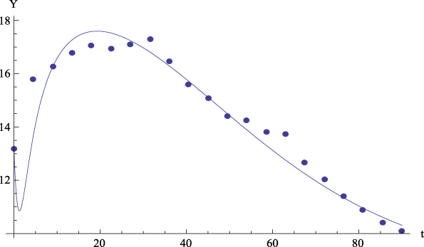
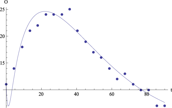
Let us comment the figures corresponding to the mean data. On the one hand, Figure 2 shows, for the average values, the plot of GFP (Y) together with the curve predicted by Equation (4) versus time. On the other hand, Figures 3 to 6 show, for the average values, respectively, the plots of Extraversion (E), Responsibility (R), Neuroticism (N), Openness to Experience (O) and Agreeableness (A), together with the curves predicted by Equation (5.i) versus time. The outcomes for the determination coefficient (R2) can be found in Table 3 and below each figure. They represent a high fitting degree between the experimental data and the theoretical curve. Only in the case of Neuroticism R2 is notably lower; data presents a certain dispersion that, however, is not present in other cases, for which this R2 is considered as high enough to be accepted as important.
Table 3. Mean data and Cases 1 to 20. Determination coefficients (R2) between the experimental data and the theoretical curve given by equations (2), (3) and (4) (for column 2), or by equations (2), (3) and (5.i), 1≤ i ≤ 5 (respectively, for columns 3 to 7)


Figure 2: Average values. Experimental data (dots) of the GFP (Y) together with the theoretical prediction (curve) from equation (4) versus time. R 2 = .94.

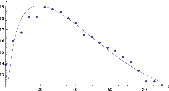
Figure 3: Average values. Experimental data (dots) of Extraversion (E) together with the theoretical prediction (curve) from equation (5.1) versus time. R 2 = .96.

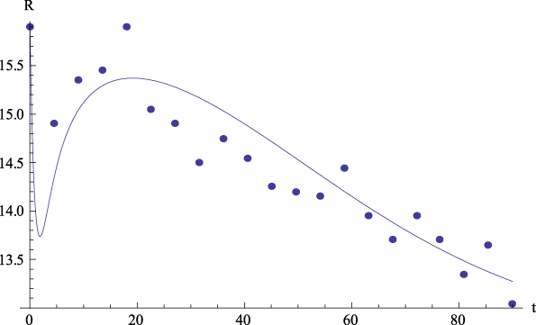
Figure 4: Average values. Experimental data (dots) of Responsibility (R) together with the theoretical prediction (curve) from equation (5.2) versus time. R 2 = .79.
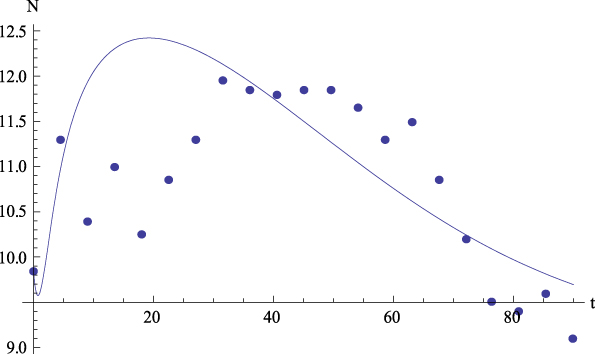
Figure 5: Average values. Experimental data (dots) of Neuroticism (N) together with the theoretical prediction (curve) from equation (5.3) versus time. R 2 = .35.

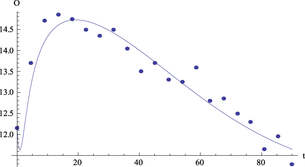
Figure 6: Average values. Experimental data (dots) of Openness to Experience (O) with the together theoretical prediction (curve) from equation (5.4) versus time. R 2 = .92.

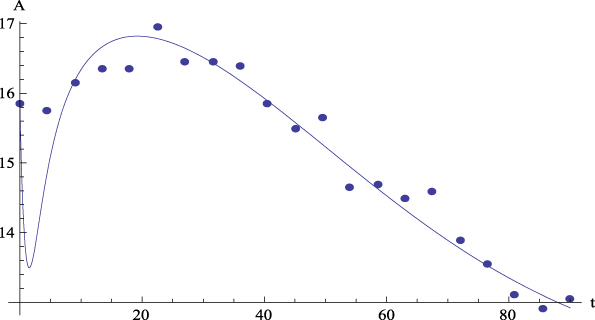
Figure 7: Average values. Experimental data (dots) of Agreeableness (A) together with the theoretical prediction (curve) from equation (5.5) versus time. R 2 = .94.
Let us now comment the figures corresponding to Case 1. On the one hand, Figure 8 shows the plot of GFP (Y) together with the curve predicted by Equation (4) versus time. On the other hand, Figures 9 to 13 show, respectively, the plots of Extraversion (E), Responsibility (R), Neuroticism (N), Openness to Experience (O) and Agreeableness (A) together with the curves predicted by Equation (5.i) versus time. The outcomes for the determination coefficients can be found in Table 3 and below each figure. They reveal a high fitting degree between the experimental data and the theoretical curve, the case of Neuroticism included, which, for this case, is significantly high.
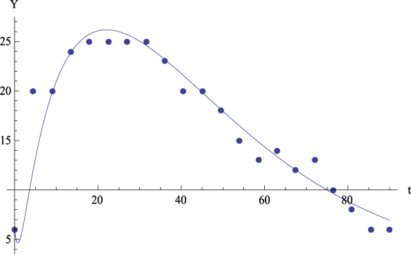
Figure 8. Case 1. Experimental data (dots) of GFP (Y) together with the theoretical prediction (curve) from equation (4) versus time. R 2 = .90.
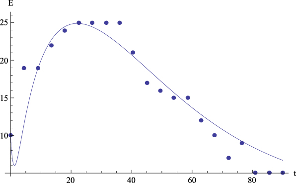
Figure 9. Case 1. Experimental data (dots) of Extraversion (E) together with the theoretical prediction (curve) from equation (5.1) versus time. R 2 = .90.

Figure 10. Case 1. Experimental data (dots) of Responsibility (R) together with the theoretical prediction (curve) from equation (5.2) versus time. R 2 = .86.
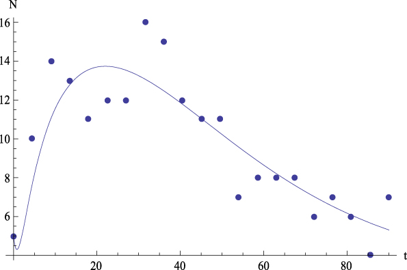
Figure 11. Case 1. Experimental data (dots) of Neuroticism (N) together with the theoretical prediction (curve) from equation (5.3) versus time. R 2 = .73.

Figure 12: Case 1. Experimental data (dots) of Openness to Experience (O) together with the theoretical prediction equation (curve) from equation (5.4) versus time. R 2 = .96.
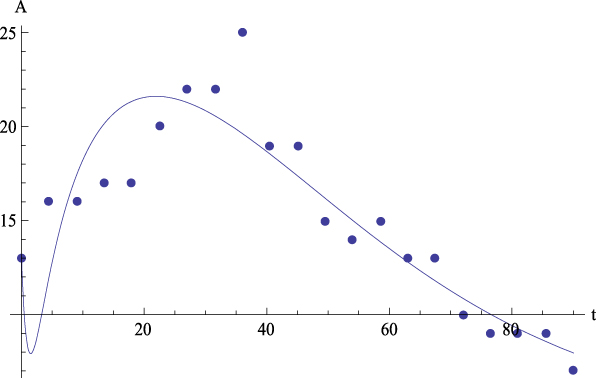
Figure 13. Case 1. Experimental data (dots) of Agreeableness (A) together with the theoretical prediction (curve) from equation (5.5) versus time. R 2 = .81.
The visual inspection of the theoretical curves together with the experimental data confirm the suitability of the response model (Equations (2), (3) and (4) or (2), (3) and (5.i), 1 ≤ i ≤ 5) to explain the data. Thus, this model describes successfully the dynamic pattern of the GFP and the B5F as a consequence of the consumption of a stimulant drug as caffeine is. The determination coefficients for all cases can be found in Table 3. Jointly viewed, they constitute a set of determination coefficients that are high enough to support this confirmation despite the fact that there are some uncorrelated cases or factors. Our hypothesis is that the uncorrelated cases or factors are due to the null effect that caffeine can produce on some individuals as a consequence of the weakness of caffeine as a stimulant drug or as a consequence of habituation in these individuals. Experiments with stimulant drugs with stronger effect perhaps provide higher determination coefficients in these cases.
An important consequence of the response model fitting to the experimental data is that, on the one hand, the model provides a general pattern to reproduce personality dynamics as a consequence of caffeine consumption, and, on the other hand, this fitting provides simultaneously knowledge about between-persons variation through the individual differences given by the particular parameter values of the response model. The individual differences can be appreciated in the particular parameter values in Table 1 (for the average data) and in Table 2 (for the Case 1 data), which are a consequence of a different individual biology.
The Bridge Model Validation
The validation of the solutions of the bridge model ((29.i), 1 ≤ i ≤ 5), has also been performed for the average data and for each one of the twenty cases. It consists on showing the good adaptation of the model to the data obtained in the experiment. The parameter values are obtained in Section 5.1. The fitting procedure has been performed again with the help of MATHEMATICA 6.0. The procedure is constituted by the following steps:
-
a. Getting the functions E i (t,y), 1 ≤ i ≤ 5, by substitution of the parameter values obtained in section 5.1. Note that α, β, a, b, p and q parameters are common to the five equations that provide each one of the B5F as a function of time and the GFP.
-
b. Plotting together the experimental values of the B5F and the computed ones by Equation (29.i) versus experimental GFP values. A complete three-dimensional plot, i.e., versus time and GFP, is not suitable to show visually the fitting degree between the experimental and the theoretical data. In addition, the determination coefficients, R2, are computed in order to quantify the fitting degree.
The results of this procedure for the average values are described in the following. Figures 14 to 18 show, respectively, the plots of Extraversion (E), Responsibility (R), Neuroticism (N), Openness to Experience (O) and Agreeableness (A), together with the values predicted by Equation (29.i) versus the GFP experimental values. The outcomes for the determination coefficients can be found in Table 4 and inside figure captions. They reveal a high fitting degree between the experimental and the theoretical data with the only exception of Neuroticism (Figure 5) were such degree is notably lower. In all the other cases the determination coefficient is high enough to be accepted as important, as it can be observed in Table 4.
Table 4. Mean data and Cases 1 to 20. Determination coefficients (R2) between the experimental data and the values given by equation (29.i), 1≤ i ≤ 5 (respectively, for columns 2 to 6)


Figure 14. Average values. Experimental data (dots) of Extraversion (E) together with the theoretical values F 1 (t,y) (triangles) from equation (29.1) versus experimental values of the GFP (Y). R 2 = .96.
Figure 15. Average values. Experimental data (dots) of Responsibility (R) together with the theoretical values F 2 (t,y) (triangles) from equation (29.2) versus experimental values of the GFP (Y). R 2 = .82.

Figure 16. Average values. Experimental data (dots) of Neuroticism (N) together with the theoretical values F 3 (t,y) (triangles) from equation (29.3) versus experimental values of the GFP (Y). R 2 = .38.
Figure 17. Average values. Experimental data (dots) of Openness to Experience (O) together with the theoretical values F 4 (t,y) (triangles) from equation (29.4) versus experimental values of the GFP (Y). R 2 = .93.

Figure 18. Average values. Experimental data (dots) of Agreeableness (A) together with the theoretical values F 5 (t,y) (triangles) from equation (29.5) versus experimental values of the GFP (Y). R 2 = .96.
The results corresponding to Case 1 appear in Figures 19 to 23 that represent respectively the plots of Extraversion (E), Responsibility (R), Neuroticism (N), Openness to Experience (O) and Agreeableness (A), together with the values predicted by Equation (29.i) versus the GFP experimental values. The corresponding determination coefficients are in Table 4 and below each figure. They reveal a high fitting degree between the experimental data and the theoretical curve (the case of Neuroticism included, which is notably high).
Figure 19. Case 1. Experimental data (dots) of Extraversion (E) together with the theoretical values F 1 (t,y) (triangles) from equation (29.1) versus experimental values of the GFP (Y). R 2 = .80.
Figure 20. Case 1. Experimental data (dots) of Responsibility (R) together with the theoretical values F 2 (t,y) (triangles) from equation (29.2) versus experimental values of the GFP (Y). R 2 = .50.
Figure 21. Case 1. Experimental data (dots) of Neuroticism (N) together with the theoretical values F 3 (t,y) (triangles) from equation (29.3) versus experimental values of the GFP (Y). R 2 = .76.

Figure 22. Case 1. Experimental data (dots) of Openness to Experience (O) together with the theoretical values F 4 (t,y) (triangles) from equation (29.4) versus experimental values of the GFP (Y). R 2 = .76.
Figure 23. Case 1. Experimental data (dots) of Agreeableness (A) together with the theoretical values F 5 (t,y) (triangles) from equation (29.5) versus experimental values of the GFP (Y). R 2 = .67.
The visual inspection of the theoretical values together with the experimental ones confirms the suitability of the model (29.i), 1 ≤ i ≤ 5, to explain the experimental results. Thus, the solutions of the bridge model (29.i) describe successfully the functional relations of the B5F with respect to time and GFP, as a consequence of a stimulant drug (caffeine) intake. The determination coefficients for all cases can be found in Table 4. Jointly viewed, they are high enough to support this confirmation despite there are some uncorrelated cases or factors. Our hypothesis about these uncorrelated cases is the same than the one exposed in Section 5.1: it is due to the null effect that caffeine can produce in some individuals as a consequence of the weakness of caffeine as a stimulant drug or as a consequence of habituation.
Discussion
A series of studies has concluded that the GFP is a common factor to the B5F and can be obtained from them (Amigó et al., Reference Amigó, Caselles and Micó2010; Musek, Reference Musek2007; Rushton & Irwing, Reference Rushton and Irwing2008; Rushton et al., Reference Rushton, Bons and Hur2008). A scheme of the structure of relations between the GFP and the B5F is obtained in this paper. Nevertheless, personality has a powerful dynamic component that is explained by the response model, as it can be observed in the results corresponding to the application case presented (see Figures 2 to 13). These results agree with the psychological and biological results of similar works such as the following ones:
-
• The work of Amigó et al., (Reference Amigó, Caselles and Micó2008), which studies the dynamic response of the brain activation level (as a biological base of the GFP) as a consequence of a generic stimulant drug intake.
-
• The work of Caselles, Micó, and Amigó (Reference Caselles, Micó and Amigó2011), which studies the dynamic response of the GFP as a consequence of an intake of caffeine.
-
• The work of Micó, Amigó, and Caselles (Reference Micó, Amigó and Caselles2012), which studies the dynamic response of the GFP and the regulator gene c-fos (as a biological base of personality) as a consequence of a dose of methylphenidate.
-
• In these three studies it is verified that the response model reproduces the dynamics of the brain activation level.
-
• The work of Amigó et al., (Reference Amigó, Caselles, Micó and García2009a) studies the temporary change of the GFP in relation to the concentration of glutamate in blood (as a biological substratum of personality) as a consequence of a dose of methylphenidate, being observed that as much the GFP as the glutamate responds to a dynamic pattern similar to the one reproduced by the response model.
-
• The work of Amigó, Caselles, and Micó (Reference Amigó, Caselles and Micó2013) studies the temporary change of the GFP in relation with the regulating gene DRD3 (like another biological substratum of personality) as a consequence of a suggestion technique, being observed that as much the GFP as the DRD3 respond to a dynamic pattern similar to the one reproduced by the response model.
In the results presented in this paper (see Figures 2 to 13), it is observed that also the response model reproduces the dynamics of the B5F. Therefore, we consider a main result of the present work the verification of the fact that the dynamics of the main aspects of personality, as a consequence of a stimulus, can be reproduced with the response model.
In addition, given the dynamic nature of personality, what we demonstrated in this article is that the bridge model quantitatively relates the GFP and the B5F. We have not found any previous study with the objective of relating the B5F from the point of view of the dynamic relations considered by the bridge model. Figures 14 to 19 show its predictive power.
On the other hand, let us recall that we left from the UPTT, whose fundamental postulate is (Amigó, Reference Amigó2005):
-
a. The UPTT proposes a hierarchical model of personality where the highest level corresponds to the GFP which includes the B5F. Nevertheless, considering the contributions of the response model and the bridge model, two new postulates of dynamic character would be needed in the UPTT base:
-
b. The GFP and the B5F have a dynamic character. This dynamics can be represented mathematically by the response model, which is valid and common to reproduce it as a consequence of a drug intake and, possibly, of any stimulus.
-
c. The evolutions of the GFP and the B5F are not independent but related. These relations can be represented mathematically by the bridge model.
Thus, following Postulates 1, 2 and 3, the UPTT can be considered as a unified dynamic theory of personality. Postulates 2 and 3 represent the co-evolution of all factors here considered, included the GFP. Postulate 2 is suggested by the results presented in this paper and the results of the works listed above, while Postulate 3 is suggested only by the results presented in this paper. The theory, in the future, should be contrasted for other types of stimuli, such as non stimulant drugs or all those related with the human senses.
The application case presented in this paper to verify Postulates 2 and 3, consists of an experimental group with twenty adult subjects that consumed coffee on an empty stomach, where the GFP and the B5F are measured by two scales of adjectives: the Big Five Personality Adjectives List (BFPAL) (Brody & Ehrlichman, Reference Brody and Ehrlichman1998) and the Five-Adjective Scale of the General Factor of Personality (GFP-FAS, Amigó et al., Reference Amigó, Micó and Caselles2009b). These ones are two scales of adjectives in state-format that are completed several times after taking the coffee. This allows making an analysis of the change and the dynamics of personality, necessary to validate the response model and the bridge model.
We can mention several limitations of this study. In the first place, and as we have already indicated, it would be advisable to repeat the study with other environmental stimuli, may be other stimulating drugs, but also with depressing drugs, for the sake of the generalization of the results and the most complete validation of the model. It would be also advisable, in future studies, to consider the previous experience of the participants with the drug that is being used, that is to say, if they are non-consumers, occasional consumers or frequent consumers. We have seen that the response model without the delay parameter can be validated for the caffeine stimulus. However, avoiding this parameter is not possible in general. For instance, the response model needs to consider the delay when the stimulus is methylphenidate (Micó et al., Reference Micó, Amigó and Caselles2012). Thus, a generalization of the bridge model that contains the delay parameter must be investigated. Obviously, it is assumed that the model is considered as a hypothesis that has resulted as validated through its contrast with real data from experience. The origins of the model have been to try to explain mathematically the biological and psychological processes previously observed by researchers and to try to extract consequences from it.
But, why is the response model chosen to fit the experimental data and not another kind of model? Because:
-
• A fundamental hypothesis of the UPTT is that personality has a dynamic character, thus a dynamic model is needed. The response model has this required dynamic character and has been validated in other contexts to evaluate personality dynamics (Amigó et al., Reference Amigó, Caselles and Micó2008; Caselles et al., Reference Caselles, Micó and Amigó2011; Micó et al., Reference Micó, Amigó and Caselles2012) (see above in this section about the discussion of these papers). Moreover, the data are observed on a time sequence (they are not static data).
-
• The response model, as a differential equation, provides quantitatively partial dynamic processes of the personality theory with biological sense, such as the homeostatic control, the excitation effect, the inhibitor effect and the stimulus. Also, the model parameters have all a biological sense (see Section 2 about the response model).
Other competitive models perhaps could fit the experimental data; for example, Structural Equations Modeling (SEM) approach, time series or network models. However:
-
• The authors consider that the response model is a consolidated knowledge, its equations and parameters have a biological sense and the bridge model can be deduced from it to relate the B5F and the GFP conserving the biological sense of the parameters. Observe that once the response model is accepted as a consolidated knowledge, the bridge model is deduced from the hypothesis that the dynamics of GFP and the B5F is invariant, i.e., their dynamics holds the response model. Thus, the bridge model is a consequence of the assumptions stated to deduce the response model. The SEM approach hardly if not impossible (we could not achieve it), can respect the causal diagram of Figure 1 with the biological sense of its parameters, concepts and structure.
-
• On the other hand, the time series and the network models are only input-output models that could not provide any explanation about the biological mechanisms of the personality dynamics, such as the homeostatic control, the excitation effect or the inhibition effect.
A final question to discuss is whether the data described are comparable or not to, for example, time-course data in the positive sciences such as physics or chemistry, when the data are measured by a machine that is not getting bored and that is capable of performing a measurement every second or even millisecond. It seems evident that the data collected in the experimental design have a greater measurement error. The authors assume that any measure has an error due to the method of measure and the device of measure. In the context of the GMM, the consideration of error in models converts them into stochastic models. The GMM contemplates two modeling possibilities: deterministic and stochastic. The stochastic models arise when either the randomness of some input variables can be deduced from a group of data or when some fitting functions are needed to obtain the model from experimental or historical data. The deterministic models arise when none of these two options is possible or necessary. When convenient, the detailed method to obtain a stochastic model can be found in the works of Caselles (Reference Caselles and Trappl1992b, Reference Caselles2008). An example of stochastic model obtained following this method in the context of social systems is the work of Sanz, Micó, Caselles, and Soler (Reference Sanz, Micó, Caselles and Soler2014). In the context of the present study, the randomness of some variables could be deduced from the person-variability in the group (which would include personal differences and measurement errors). However, this approach should be a future work, when more deterministic approaches consolidate the model.
In general, the response model and the bridge model open a way to be followed in a future time, not only with psychological instruments, but with measures of biological character that provide a better understanding of the dynamic and biological nature of the human personality.
An epistemological limitation of the presented formalism is that the response and bridge models can turn out too complex to be used in Psychological research. But we want here to break a lance in favor of the contribution of the General Systems Theory to expand the horizon of research. In the context of this trans-disciplinary vocation, the research has got together psychologists, mathematicians and physicists who have collaborated very closely. This collaboration has allowed elaborating the response model like a system of three connected differential equations, and the bridge model like a partial derivative equation, contributing of this way to give an epistemological status to Personality Theory similar to that of applied sciences, such as it is asserted in the introduction of this paper. This article is a clear bet for the inter-disciplinary study of high level, and the result has been to enrich the UPTT with two new postulates of dynamic character.
This article offers the possibility of integrating in a high level important theoretical and methodological aspects like:
-
a. The structural perspective of personality as opposed to the dynamic one.
-
b. The perspective of trait as opposed to the one of state in the studies of personality (it has been used here lists of adjectives in state-format).
-
c. The study of the basic components of personality as opposed to the global and holistic conception of the same one (represented by the GFP).
-
d. The experimental study of personality on the one hand, and on the other one, the elaboration of two complex mathematical models based on the Theory of Systems.
-
e. The internalist perspective of personality as opposed to the environmentalist perspective (represented by the changes of personality in response to a drug intake).
These complex mathematical models (the response model and the bridge model), will allow us to describe personality in all its complexity and to predict its changes in response to environmental stimuli, as it can be the consumption of a drug. Thus, as much from a theoretical point of view as from an applied one, the models here proposed open a new perspective in the understanding and study of personality like a global system that interacts intimately with the environment. As we above said, this study is a clear bet for the high level inter-disciplinary research, a bet that will have to be perfected but that it is very important so that the future science is based on the integration of the human knowledge.
We thank very much the Department of Analytical Chemistry of the Universitat de València, Spain, for the help with the analysis of the caffeine concentration in the coffee used in the experiment.