


1 Introduction
Silicon is produced in submerged arc furnaces by reducing quartz rock (
 $\textrm{SiO}_2$
) with carbon. The energy required for the highly endothermic chemical reactions that take place in the furnace is provided by passing an electric current through the raw and partially reacted materials (known as the charge material) between the electrodes and the base of the furnace. This current is mostly carried by an electric arc through a gas-filled cavity (the crater) that forms beneath each electrode, but some current is also conducted through the charge material, in parallel with the arc [Reference Schei, Tuset and Tveit42]. A drawing of the silicon furnace showing two electrodes, with craters at the base of each, is shown on the left of Figure 1. Since the electric current causes Ohmic heating, understanding the distribution of current between these two parallel current paths is important in order to understand the chemical processes, which are highly temperature-dependent. In particular, a poor current distribution – with too much current through the charge material and not enough through the arc – can develop suddenly and is seen in practice to cause inefficient silicon production, although it is not well understood what causes this change in the current distribution [Reference Schei, Tuset and Tveit42].
$\textrm{SiO}_2$
) with carbon. The energy required for the highly endothermic chemical reactions that take place in the furnace is provided by passing an electric current through the raw and partially reacted materials (known as the charge material) between the electrodes and the base of the furnace. This current is mostly carried by an electric arc through a gas-filled cavity (the crater) that forms beneath each electrode, but some current is also conducted through the charge material, in parallel with the arc [Reference Schei, Tuset and Tveit42]. A drawing of the silicon furnace showing two electrodes, with craters at the base of each, is shown on the left of Figure 1. Since the electric current causes Ohmic heating, understanding the distribution of current between these two parallel current paths is important in order to understand the chemical processes, which are highly temperature-dependent. In particular, a poor current distribution – with too much current through the charge material and not enough through the arc – can develop suddenly and is seen in practice to cause inefficient silicon production, although it is not well understood what causes this change in the current distribution [Reference Schei, Tuset and Tveit42].

Figure 1. Left: a drawing of an industrial silicon furnace [Reference Hannesson19], showing a crater at the base of each of the electrodes, and the red square highlighting the area modelled. Right: sketch of the problem domain (top), idealised geometry consisting of nested cylinders (center), and detail illustrating the change of coordinates (2.1) and the changing volume fractions of solid and gas across the thin reacting layer of charge material (bottom).
While the electrical current generates heat by Ohmic heating, the electrical conductivities of both the arc and the charge material increase with temperature, meaning that the thermal and electrical effects are fully coupled. The heat transfer in the furnace must therefore be considered in order to understand the current distribution. Since the charge material is only electrically conductive at very high temperatures near the crater, we restrict our attention to the region surrounding the crater, as shown in Figure 1. Heat is transferred from the arc to the charge material surrounding the crater by radiation and through the flow of hot gases out of the crater through the porous charge material. Energy is absorbed in the charge material through chemical reactions, which alter the composition of the charge. Although there are many reactions, a reasonable simplistic model is that these reactions convert the solid charge materials to gases. These gases then undergo further, less energy-intensive reactions to produce the liquid silicon. As solid material is consumed, more material flows in towards the crater. The position of the interface between the crater and charge material may therefore be modelled as a free boundary, determined by a balance of the material inflow and consumption by chemical reactions, and thus, like these processes, is coupled to the thermal and electrical problem.
There are a number of detailed models for the chemical processes, material flow and heat transfer within silicon furnaces, including those presented in [Reference Andresen1, Reference Scheepers, Adema, Yang and Reuter41]. Due to the heavy coupling between these processes, both [Reference Andresen1, Reference Scheepers, Adema, Yang and Reuter41] rely on commercial computational fluid dynamics (CFD) packages to simulate the behaviour. A mathematical approach is taken in the thesis [Reference Sloman45] and the related papers [Reference Sloman, Please and Van Gorder46, Reference Sloman, Please and Van Gorder47, Reference Sloman, Please, Van Gorder, Valderhaug, Birkeland and Wegge49], which provide detailed analysis of the changing material compositions in the different regions of the furnace. This includes modelling and analysis of the formation of a crust in the charge material, as well as models for the fine scale chemical processes which are then homogenised to describe an overall bulk reaction. However, none of these studies take into account the effect of the electric current on the process: the models in [Reference Sloman45] are for a laboratory scale pilot furnace which is heated by an induction furnace, while [Reference Scheepers, Adema, Yang and Reuter41] do not model the electric current at all. In [Reference Andresen1], the electric current in the arc is included, with a prescribed current distribution, and it is assumed that the current has little effect on the processes elsewhere in the furnace. Conversely, models for the electric current throughout the furnace rarely couple the current distribution to the thermal problem in a meaningful way. For instance [Reference Bermúdez, Muñiz, Pena and Bullón4, Reference Dhainaut13, Reference Tesfahunegn, Magnusson, Tangstad and Sævarsdóttir50] solve for the current density in the furnace, with [Reference Bermúdez, Muñiz, Pena and Bullón4] also taking magnetic effects into account. The electrical conductivities of the different regions in the furnace are prescribed constants in all of these studies, so that there is no coupling between the electrical and thermal problems. Other studies, including [Reference Budd, Jones, Biesenbach and Halvorsen9, Reference Sævarsdóttir and Bakken40, Reference Valderhaug52], model the furnace as an electric circuit, with the electrical properties modelled using lumped voltages, currents, resistances and inductances, which are related using Kirchhoff’s laws. Skin and proximity effects between the different electrodes and the casing of the furnace are analysed in [Reference Herland, Sparta and Halvorsen20]. Again, the thermal problem is not considered in these models, so there is no capacity for positive current–temperature feedback.
In this paper, we model the coupled electrical and thermal processes in a simplified geometry representing the region surrounding an electrode in a silicon-producing furnace, including the flow and consumption of the charge material by chemical reactions, and the flow of the gases produced by these reactions both in the charge and in the crater. Accounting for these couplings allows us to explore the mechanisms affecting the current distribution between the arc and charge material. The paper is structured as follows. In Section 2, we derive a model for the coupled electric current and heat transfer between the electric arc and the charge material and nondimensionalise using industrially relevant parameter values. We then homogenise our model over the timescale of the alternating current in Section 3, further simplifying the model by taking a quasi-steady limit. In Section 4, we solve our quasi-steady, homogenised model. We first look in detail at the fast-timescale variation of the electric field and arc temperature predicted by our arc model, comparing the solutions qualitatively with industrial measurements and existing models. We then present numerical solutions of the full homogenised model in Section 4.2. The existence of steady-state solutions and the evolution of the system are discussed in relation to the overall balance of energy in Section 4.3. We also relate the qualitative behaviour of these solutions to the furnace behaviour observed in practice. Discussion of the model behaviour and implications for industrial silicon production are presented in Section 5.
2 Derivation of the submerged arc furnace model
We are interested in the distribution of current between the electric arc and the charge material surrounding the crater, which is fully coupled to the heat transfer between and within these regions, and also to the chemical reactions in the charge material. We therefore consider the conservation of energy in the arc, as well as the conservation of mass and energy of the solid and gaseous material in the charge, lumping all chemical species into just one solid and one gaseous phase. The arc and charge regions are coupled thermally by the radiative heat transfer between the arc and the solid surfaces of the crater, and electrically by both Kirchhoff’s law, and by imposing a total current through the system.
2.1 Idealised geometry
We only model the region surrounding the base of a single electrode in a submerged arc furnace. We consider a highly simplified geometry consisting of axisymmetric nested cylinders for the electric arc, crater and charge material, as illustrated on the bottom right of Figure 1. We use polar coordinates (r,z) and prescribe a height h of our domain, corresponding to the height of the electrode from the base of the crater.
The electric arc is assumed to form at the centre of the crater, about
 $r=0$
, and is contained in a cylinder of prescribed radius
$r=0$
, and is contained in a cylinder of prescribed radius
 $r_a$
. The crater/charge interface at
$r_a$
. The crater/charge interface at
 $r=s(t)$
will be a free boundary in our model. We assume that
$r=s(t)$
will be a free boundary in our model. We assume that
 $s(t)\gg r_a$
. The charge material forms an annulus around the crater in
$s(t)\gg r_a$
. The charge material forms an annulus around the crater in
 $r\geq s(t)$
. We assume that only a thin layer of the charge material immediately surrounding the crater is hot enough to be electrically conductive. We therefore restrict our attention to this thin annulus of charge material, by changing variables, setting
$r\geq s(t)$
. We assume that only a thin layer of the charge material immediately surrounding the crater is hot enough to be electrically conductive. We therefore restrict our attention to this thin annulus of charge material, by changing variables, setting
 \begin{equation}r=s(t)+ X\,,\end{equation}
where
 $X\ll s$
, so that the thin layer of charge material consists of the region
$X\ll s$
, so that the thin layer of charge material consists of the region
 $X\in[0,\infty)$
.
$X\in[0,\infty)$
.
2.2 Modelling of the electric arc
The electric arc is a continuous gas discharge, where the gas is ionised into a plasma of electrons and ions which carry the electric current. The flow of current through the arc generates heat by Ohmic heating. At higher temperatures, the ionisation of the plasma is greater, so that the electrical conductivity of the arc increases with temperature.
The term ‘electric arc’ covers a wide variety of phenomena. As described by [Reference Jones and Fang25, Reference Valderhaug52], the furnace arcs are ‘high pressure’ (in comparison with vacuum arcs), in that they are at approximately atmospheric pressure. They are ‘free-burning’ in the sense that they are not confined to be within a narrow region (compared with ‘wall-constrained’ arcs, the subject of much of the arc literature and described in [Reference Jones and Fang25]). Finally the arc is ‘thermal’, with its shape and size self-determined by a balance of heat generation and transfer to the surroundings [Reference Bakken, Gu, Larsen and Sevastyanenko3, Reference Pfender35, Reference Valderhaug52]. The high current through the arc generates a strong magnetic field, so that a Lorentz force is exerted on the ionised gases. This generates a plasma flow axially along the electric arc from cathode to anode that can reach velocities of around
 $500\ \textrm{ms}^{-1}$
[Reference Andresen1], so that the gas flow has an important effect on the temperature distribution through convection, and the movement of the charged material in the magnetic field induces a secondary current.
$500\ \textrm{ms}^{-1}$
[Reference Andresen1], so that the gas flow has an important effect on the temperature distribution through convection, and the movement of the charged material in the magnetic field induces a secondary current.
There are many different models for arcs of this type. The complicated flow, heat transfer and electromagnetic forces within the arc may be captured by magnetohydrodynamic (MHD) models, such as those used in [Reference Sævarsdóttir39, Reference Thompson, Richardson, Dellar, McGuinness and Budd51]. However, the complexity of MHD arc models makes them impractical to include in our model of the overall current distribution in the furnace. Many empirical models are also used to describe electric arcs. For instance [Reference Bowman and Krüger5] gives an overview for arcs in open-arc steelmaking furnaces, which have many similarities with those occurring in submerged-arc furnaces. Other studies such as [Reference Budd, Chapman, Lacey and Ockendon8, Reference Cowley11, Reference Lago, Gonzalez, Freton and Gleizes30, Reference Lowke31, Reference Pfender35, Reference Ramakrishnan, Stokes and Lowke36, Reference Schlitz, Garimella and Chan43, Reference Wang, Liu, Gong, Li and Ma53] use simplified physics-based models for the arc. These model the arc as a cylindrical region with a purely axial electric current and do not include any effects due to the magnetic field. The temperature within this cylindrical arc is affected by Ohmic heating, and heat losses that may include radiation, convection and conduction. Specific examples include the Cassie, and Mayr models, described in [Reference Gustavsson17], for which heat loss from the arc is an approximation of purely convective and purely conductive, respectively.
For simplicity, we choose to use a simplified-physics model. Within the arc region
 $0<r<r_a$
, we suppose that the electric current is vertical and is unaffected by magnetic fields, so that the arc current
$0<r<r_a$
, we suppose that the electric current is vertical and is unaffected by magnetic fields, so that the arc current
 $\boldsymbol{J}_a$
is given by Ohm’s law,
$\boldsymbol{J}_a$
is given by Ohm’s law,
 $\boldsymbol{J}_a=\sigma_a(T_a)E_a \boldsymbol{e}_z,$
where
$\boldsymbol{J}_a=\sigma_a(T_a)E_a \boldsymbol{e}_z,$
where
 $E_a$
is the (vertical) electric field strength and
$E_a$
is the (vertical) electric field strength and
 $\sigma_a(T_a)$
is the electrical conductivity of the arc, which depends strongly on the temperature
$\sigma_a(T_a)$
is the electrical conductivity of the arc, which depends strongly on the temperature
 $T_a$
, which we assume is uniform throughout the arc.
$T_a$
, which we assume is uniform throughout the arc.
The Cassie model assumes a constant arc conductivity (although a varying arc radius), while the Mayr model assumes an exponential dependence of
 $\sigma_a$
on
$\sigma_a$
on
 $T_a$
[Reference Gustavsson17]. We use the functional form
$T_a$
[Reference Gustavsson17]. We use the functional form
 \begin{equation}\sigma_a(T_a)=S_1 \exp\left(-\frac{S_2}{T_a}\right)\end{equation}
suggested in [Reference Hoyaux23], with constants
 $S_1=2.5\times 10^4\,\textrm{S}\,\textrm{m}^{-1}$
and
$S_1=2.5\times 10^4\,\textrm{S}\,\textrm{m}^{-1}$
and
 $S_2=1.8\times 10^4\,\textrm{K}$
, chosen to give reasonable qualitative agreement with the data shown in [Reference Sævarsdóttir39] for the crater gas of a silicon-producing furnace. We note that the exponential dependence of
$S_2=1.8\times 10^4\,\textrm{K}$
, chosen to give reasonable qualitative agreement with the data shown in [Reference Sævarsdóttir39] for the crater gas of a silicon-producing furnace. We note that the exponential dependence of
 $\sigma_a$
on
$\sigma_a$
on
 $T_a$
used in the Mayr model is an approximation of (2.2) in the case where the variation in
$T_a$
used in the Mayr model is an approximation of (2.2) in the case where the variation in
 $T_a$
is small, and thus the two forms for the conductivity agree over a small range of
$T_a$
is small, and thus the two forms for the conductivity agree over a small range of
 $T_a$
.
$T_a$
.
Neglecting displacement currents [Reference Davidson12], the current satisfies the conservation of charge constraint
 \begin{equation}{\frac{\partial}{\partial{z}}} \left( \sigma_a(T_a)E_a)\right)=0.\end{equation}
Since the temperature
 $T_a$
is uniform throughout the arc, (2.3) implies that
$T_a$
is uniform throughout the arc, (2.3) implies that
 $E_a(t)$
is also uniform.
$E_a(t)$
is also uniform.
We assume that the temperature
 $T_a$
within
$T_a$
within
 $0<r<r_a$
depends on the Ohmic heating, which produces energy
$0<r<r_a$
depends on the Ohmic heating, which produces energy
 $\boldsymbol{J}_a\cdot\boldsymbol{E}_a$
per unit volume. We also suppose that the dominant heat loss from the arc is due to radiation, and furthermore that the gas is optically thin to the radiation, so that none of the radiation is reabsorbed within the arc or surrounding crater gas, but is instead incident on the crater walls. In this case, the energy,
$\boldsymbol{J}_a\cdot\boldsymbol{E}_a$
per unit volume. We also suppose that the dominant heat loss from the arc is due to radiation, and furthermore that the gas is optically thin to the radiation, so that none of the radiation is reabsorbed within the arc or surrounding crater gas, but is instead incident on the crater walls. In this case, the energy,
 $\mathcal{R}$
, lost to radiation per unit volume within the arc is [Reference Modest32],
$\mathcal{R}$
, lost to radiation per unit volume within the arc is [Reference Modest32],
 $\mathcal{R}=4a\sigma_BT_a^4,$
where
$\mathcal{R}=4a\sigma_BT_a^4,$
where
 $\sigma_B=5.7\times 10^{-8}\,\textrm{W}\,\textrm{m}^{-2}\,\textrm{K}^{-4}$
is the Stefan–Boltzmann constant, and a is the absorption coefficient. This absorption coefficient generally depends on both temperature and pressure [Reference Modest32] but, for simplicity, we take
$\sigma_B=5.7\times 10^{-8}\,\textrm{W}\,\textrm{m}^{-2}\,\textrm{K}^{-4}$
is the Stefan–Boltzmann constant, and a is the absorption coefficient. This absorption coefficient generally depends on both temperature and pressure [Reference Modest32] but, for simplicity, we take
 $a= 0.1\,\textrm{m}^{-1}$
to be constant (using the approximate value for CO gas [Reference Rivière and Soufiani37]). The energy emitted in this way must then be accounted for at the solid boundaries of the crater domain, which we discuss in Section 2.4.2. In reality, the crater gas and arc plasma are not fully optically thin, and some fraction of the radiation is reabsorbed in the arc and surrounding gas [Reference Valderhaug52]. However, the radiation problem in this case quickly becomes very complicated, and so for simplicity we follow [Reference Andresen1, Reference Thompson, Richardson, Dellar, McGuinness and Budd51] and make the optically thin assumption. Within the arc the equation of conservation of energy is therefore given by
$a= 0.1\,\textrm{m}^{-1}$
to be constant (using the approximate value for CO gas [Reference Rivière and Soufiani37]). The energy emitted in this way must then be accounted for at the solid boundaries of the crater domain, which we discuss in Section 2.4.2. In reality, the crater gas and arc plasma are not fully optically thin, and some fraction of the radiation is reabsorbed in the arc and surrounding gas [Reference Valderhaug52]. However, the radiation problem in this case quickly becomes very complicated, and so for simplicity we follow [Reference Andresen1, Reference Thompson, Richardson, Dellar, McGuinness and Budd51] and make the optically thin assumption. Within the arc the equation of conservation of energy is therefore given by
 \begin{equation}\rho_a c_{p,a}{\frac{\partial{T_a}}{\partial{t}}}=\sigma_a(T_a)E_a^2-4a\sigma_BT_a^4,\end{equation}
where
 $\rho_a$
is the density, and
$\rho_a$
is the density, and
 $c_{p,a}$
is the specific heat capacity of the plasma, both assumed to be constant.
$c_{p,a}$
is the specific heat capacity of the plasma, both assumed to be constant.
Although the fluid velocity in the arc column is large, as the fluid circulates away from the arc (transferring heat away) the velocities are much slower. For instance, the CFD simulations of a MHD arc model in [Reference Andresen1] find velocities on the order of
 $10\,\textrm{m}\,\textrm{s}^{-1}$
partway between the arc and the charge, and only around
$10\,\textrm{m}\,\textrm{s}^{-1}$
partway between the arc and the charge, and only around
 $1\,\textrm{m}\,\textrm{s}^{-1}$
when it reaches the charge. Thus, we estimate the convective heat transfer from the arc to its surroundings to be
$1\,\textrm{m}\,\textrm{s}^{-1}$
when it reaches the charge. Thus, we estimate the convective heat transfer from the arc to its surroundings to be
 $\rho_a c_{p,a} v [T_a]/x\approx 10^6-10^7\,\text{W}\,\text{m}^{-3}$
, using the data in Tables 1 and 2 below, and taking a lengthscale
$\rho_a c_{p,a} v [T_a]/x\approx 10^6-10^7\,\text{W}\,\text{m}^{-3}$
, using the data in Tables 1 and 2 below, and taking a lengthscale
 $x=0.1\,$
m, and a velocity v between 1 and
$x=0.1\,$
m, and a velocity v between 1 and
 $10\,\textrm{m}\,\textrm{s}^{-1}$
. The convective heat loss is therefore likely to be smaller than the heat radiation from the arc, which, again using the data in Tables 1 and 2, is
$10\,\textrm{m}\,\textrm{s}^{-1}$
. The convective heat loss is therefore likely to be smaller than the heat radiation from the arc, which, again using the data in Tables 1 and 2, is
 $4 a\sigma_B[T_a]^4\approx 10^8\,\text{W}\,\text{m}^{-3}$
. This provides a justification for our assumption that the dominant heat-loss mechanism is radiation.
$4 a\sigma_B[T_a]^4\approx 10^8\,\text{W}\,\text{m}^{-3}$
. This provides a justification for our assumption that the dominant heat-loss mechanism is radiation.
2.3 Conservation laws in the charge material
The solid charge material consists of a mixture of carbon (C) in the form of coal and woodchips and quartz rock (
 $\textrm{SiO}_2$
), as well as silicon carbide (SiC). The structure is highly porous, so that the gases CO and SiO produced by the reactions can easily flow through the charge material. The solid materials are used up in the silicon production process, and so there is an overall flow of the solid material in towards the crater, while we expect a net flow of gas back out through the porous charge material as it is produced in and near the crater [Reference Schei, Tuset and Tveit42].
$\textrm{SiO}_2$
), as well as silicon carbide (SiC). The structure is highly porous, so that the gases CO and SiO produced by the reactions can easily flow through the charge material. The solid materials are used up in the silicon production process, and so there is an overall flow of the solid material in towards the crater, while we expect a net flow of gas back out through the porous charge material as it is produced in and near the crater [Reference Schei, Tuset and Tveit42].
2.3.1 Electric current through the charge material
The raw materials of coal, woodchips and quartz rock have negligibly small electrical conductivity at low temperatures, so we expect no current conduction high up in the furnace [Reference Schei, Tuset and Tveit42]. As the carbon materials are heated near the crater, they become partially graphitised, increasing their electrical conductivity, as described in [Reference Eidem14]. Silicon carbide, which is also electrically conductive, is formed in the furnace reactions. Since these chemical reactions require high temperatures, we only expect large quantities of SiC near the hot crater. The overall electrical conductivity of the charge material therefore depends on the temperature and chemical composition. A number of experimental studies for the electrical conductivity of the overall charge material are summarised in [Reference Valderhaug52], although studies of the functional dependence of the conductivity on temperature and material composition are limited. Since the concentration of electrically conductive materials increases with temperature, we model the conductivity as a function of temperature
 $T_s$
of the solid material only, and use the following form for the overall electrical conductivity of the charge material
$T_s$
of the solid material only, and use the following form for the overall electrical conductivity of the charge material
 \begin{equation} \sigma_c(T_s)=\begin{cases}S_c\exp\left(-\frac{E_\sigma}{T_s-T_c}\right), & \text{ for }T_s>T_c,\\ 0, & \text{ otherwise}, \end{cases}\end{equation}
for constants
 $S_c,E_\sigma>0$
and critical temperature
$S_c,E_\sigma>0$
and critical temperature
 $T_c$
. As described in [Reference Eidem14], the conductivity of the carbon materials increases significantly for temperatures above around
$T_c$
. As described in [Reference Eidem14], the conductivity of the carbon materials increases significantly for temperatures above around
 $T_c=2300\,\textrm{K}$
. From [Reference Tesfahunegn, Magnusson, Tangstad and Sævarsdóttir50], the maximum charge conductivity is expected to be on the order of
$T_c=2300\,\textrm{K}$
. From [Reference Tesfahunegn, Magnusson, Tangstad and Sævarsdóttir50], the maximum charge conductivity is expected to be on the order of
 $400\,\textrm{S}\,\textrm{m}^{-1}$
, which we take as the value of
$400\,\textrm{S}\,\textrm{m}^{-1}$
, which we take as the value of
 $S_c$
. In [Reference Mrozowski33], the conductivity of carbon increases with heat treatment, but is bounded for large temperatures. For qualitative agreement, we use
$S_c$
. In [Reference Mrozowski33], the conductivity of carbon increases with heat treatment, but is bounded for large temperatures. For qualitative agreement, we use
 $E_\sigma=300\,\textrm{K}$
.
$E_\sigma=300\,\textrm{K}$
.
We note that liquid silicon is also present in the charge material very close to the crater and is electrically conductive. However, it has extremely low viscosity and flows easily out of the porous charge structure into the crater, and so is unlikely to be the main conductor in the charge. As a simplification, we do not include the liquid silicon in our model of the overall electrical conductivity of the charge material.
We assume that the electric current is vertical in the thin layer adjacent to the crater in the conductive charge material, and so the current density
 $\boldsymbol{J}_c$
through the charge material can be given by Ohm’s law,
$\boldsymbol{J}_c$
through the charge material can be given by Ohm’s law,
 $\boldsymbol{J}_c=\sigma_c(T_s)E_c\boldsymbol{e}_z,$
where
$\boldsymbol{J}_c=\sigma_c(T_s)E_c\boldsymbol{e}_z,$
where
 $E_c$
is the vertical electric field across the charge material. Then the equation of conservation of charge is
$E_c$
is the vertical electric field across the charge material. Then the equation of conservation of charge is
 \begin{equation}{\frac{\partial{}}{\partial{z}}}\left(\sigma_c(T_s)E_c\right)=0.\end{equation}
2.3.2 Chemical reactions and conservation of mass
The chemical reactions within the charge material are a complicated system, analysed in detail in [Reference Sloman, Please and Van Gorder46]. Since we are most interested in the heat transfer through the solid materials, the consumption of these solid materials near the edge of the crater, and the consumption of heat in the endothermic reactions, we make use of the highly simplified chemical problem shown in [Reference Sloman, Please and Van Gorder46] to be a sensible reduction in the case of a pilot furnace. This simplification reduces the chemical process to just the two reactions
 \begin{align}\text{SiO}_2(\text{s})&\rightarrow\text{SiO}_2(\text{l}), \end{align}
 \begin{align}\text{SiO}_2(\text{l})+\text{C(s)}&\rightarrow \text{SiO(g)} + \text{CO(g)}.\end{align}
The SiO produced in (2.7b) then undergoes further reactions within the charge material, decomposing into Si and
 $\textrm{SiO}_2$
, or reacting with silicon carbide, to form liquid silicon [Reference Schei, Tuset and Tveit42, Reference Sloman, Please and Van Gorder46]. Some SiO also escapes out of the top of the charge material, although this is then used to create microsilica, as modelled in [Reference González-Fariña, Münch, Oliver and Van Gorder16]. It is shown in [Reference Sloman, Please and Van Gorder46] that the reactions given in (2.7) are the mechanisms by which the majority of the raw materials are vapourised (in the pilot furnace, at least). The consumption of the solid raw materials is the most endothermic part of the silicon production process [Reference Kadkhodabeigi26].
$\textrm{SiO}_2$
, or reacting with silicon carbide, to form liquid silicon [Reference Schei, Tuset and Tveit42, Reference Sloman, Please and Van Gorder46]. Some SiO also escapes out of the top of the charge material, although this is then used to create microsilica, as modelled in [Reference González-Fariña, Münch, Oliver and Van Gorder16]. It is shown in [Reference Sloman, Please and Van Gorder46] that the reactions given in (2.7) are the mechanisms by which the majority of the raw materials are vapourised (in the pilot furnace, at least). The consumption of the solid raw materials is the most endothermic part of the silicon production process [Reference Kadkhodabeigi26].
It is shown in [Reference Sloman, Please and Van Gorder46] that the rate of melting of the quartz (2.7a) is likely to be around 10 times slower than that of reaction (2.7b), and so the reaction (2.7b) is limited by (2.7a). Thus, we reduce the system to only the four chemical species,
 $\textrm{SiO}_2$
(s), C(s), SiO(g) and C(g), related by the reaction
$\textrm{SiO}_2$
(s), C(s), SiO(g) and C(g), related by the reaction
 \begin{equation}\text{SiO}_2(\text{s})+\text{C(s)}\rightarrow \text{SiO(g)} + \text{CO(g)},\end{equation}
with reaction rate that of (2.7a). Since the solid materials are consumed in a 1:1 molar ratio by (2.8), and the gases likewise are produced in a 1:1 ratio, we make the further simplification of modelling only two phases: solid and gas. In order for this assumption to make sense, we require that the raw materials fed into the furnace are also in a 1:1 molar ratio of carbon and quartz molecules.
This simplified chemical system (2.8) is based on the analysis in the case of a pilot furnace [Reference Sloman, Please and Van Gorder46], which neglects the effect of silicon carbide (SiC), in particular of the reaction [Reference Schei, Tuset and Tveit42]
 \begin{equation}2\text{SiO}_2(l)+\text{SiC}(s)\rightleftharpoons 3\text{SiO}(g)+\text{CO}(g).\end{equation}
The forward, gas-producing reaction (2.9), like reaction (2.8), is endothermic [Reference Kadkhodabeigi26]. This reaction (2.9) may in fact be important in an industrial-scale submerged arc furnace: furnace excavations have uncovered large amounts of SiC surrounding the electrodes [Reference Schei, Tuset and Tveit42]. Nevertheless, the reaction (2.8) captures the fundamental behaviour of solid material undergoing endothermic reactions to produce gases and provides a significant simplification over the full chemical system studied in [Reference Sloman, Please and Van Gorder46], therefore keeping our model tractable. As in [Reference Sloman45], we consider the charge material in the framework of multiphase flow. The solid and gas materials have within-phase densities
 $\rho_s$
and
$\rho_s$
and
 $\rho_g$
, molar concentrations over the entire medium
$\rho_g$
, molar concentrations over the entire medium
 $C_s$
and
$C_s$
and
 $C_g$
(with units
$C_g$
(with units
 $\textrm{mol}\,\textrm{m}^{-3}$
) and occupy volume fractions
$\textrm{mol}\,\textrm{m}^{-3}$
) and occupy volume fractions
 $\theta_s$
and
$\theta_s$
and
 $\theta_g$
, respectively. The velocity of the gas is
$\theta_g$
, respectively. The velocity of the gas is
 $u_g\boldsymbol{e}_r$
, which is assumed to be radial, with
$u_g\boldsymbol{e}_r$
, which is assumed to be radial, with
 $u_g$
to be determined as part of the solution.
$u_g$
to be determined as part of the solution.
To determine the velocity of the solid material, we should consider the conservation of momentum in the solid phase, as well as the conservation of mass. The gas is unlikely to significantly affect the solid flow, and so we might model the solid material as a granular fluid, using constitutive laws for the visco-plastic flow of cohesionless granular materials [Reference Forterre and Pouliquen15]. As the charge material becomes hot, the quartz becomes sticky, while the carbon particles remain solid. Constitutive laws for the flow of cohesive granular materials are less well studied [Reference Forterre and Pouliquen15], and while constitutive laws for granular flow through a viscous fluid [Reference Boyer, Guazzelli and Pouliquen6] might be appropriate, it is unclear how the hot/sticky and cold/dry regimes might be reconciled. A simpler approach would be to simply model the solid charge material as highly viscous fluid, with temperature-dependent viscosity, as in [Reference Sloman45]. Any such attempt to solve for the solid velocity would add considerable complexity to the model, by introducing additional coupling between the temperature and flow fields.
For simplicity, we instead choose to prescribe the (purely radial) velocity of the solid material to be
 $-u/r$
, for a prescribed constant u. Thus, in the absence of chemical reactions, the inward mass flux is conserved. In our thin layer
$-u/r$
, for a prescribed constant u. Thus, in the absence of chemical reactions, the inward mass flux is conserved. In our thin layer
 $X\in[0,\infty)$
, the velocity in the X direction is therefore
$X\in[0,\infty)$
, the velocity in the X direction is therefore
 $-u/s$
plus a small correction, which we neglect for simplicity, so that the solid velocity within the domain is uniform. As the material reacts away, the concentration
$-u/s$
plus a small correction, which we neglect for simplicity, so that the solid velocity within the domain is uniform. As the material reacts away, the concentration
 $C_s$
decreases, so that the porosity of the medium increases.
$C_s$
decreases, so that the porosity of the medium increases.
In our coordinate system (2.1), the two equations of conservation of mass for the solid and gas respectively are
 \begin{align}&{\frac{\partial{C_s}}{\partial{t}}}-\left(\frac{u}{s}+\dot{s}\right){\frac{\partial{C_s}}{\partial{X}}}=-\mathcal{Q},\end{align}
 \begin{align}&{\frac{\partial{C_g}}{\partial{t}}}+{\frac{\partial{}}{\partial{X}}}\big((u_g-\dot{s})C_g\big)=\mathcal{Q},\end{align}
where
 $\frac{1}{2}\mathcal{Q}$
is the rate of reaction of (2.7a), as this limits the reaction (2.8). As in [Reference Sloman45], this reaction rate increases with temperature above a certain critical temperature, below which it vanishes. The impure quartz begins to soften for temperatures above
$\frac{1}{2}\mathcal{Q}$
is the rate of reaction of (2.7a), as this limits the reaction (2.8). As in [Reference Sloman45], this reaction rate increases with temperature above a certain critical temperature, below which it vanishes. The impure quartz begins to soften for temperatures above
 $1500\,\textrm{K}$
[Reference Schei, Tuset and Tveit42]. While [Reference Sloman45] used a piecewise linear reaction rate, we choose a piecewise Arrhenius form for
$1500\,\textrm{K}$
[Reference Schei, Tuset and Tveit42]. While [Reference Sloman45] used a piecewise linear reaction rate, we choose a piecewise Arrhenius form for
 $\mathcal{Q}$
, so that it is bounded for large temperatures, namely
$\mathcal{Q}$
, so that it is bounded for large temperatures, namely
 \begin{equation}\mathcal{Q}(C_s,T_s)=\begin{cases}k_\mathcal{Q}C_s \exp\left( -\frac{E_\mathcal{Q}}{RT_s}\right), & T_s>T_m+\theta_m,\\[2mm]k_\mathcal{Q}C_s\exp\left( -\frac{E_\mathcal{Q}}{R(T_m+\theta_m)}\right)\frac{(T_s-T_m)}{\theta_m}, & T_m<T_s\leq T_m+\theta_m,\\0, & T_s<T_m.\end{cases}\end{equation}
Here
 $T_s$
is the temperature of the solid material, and
$T_s$
is the temperature of the solid material, and
 $R=8.314\,\textrm{J}\,\textrm{mol}^{-1}\,\textrm{K}^{-1}$
is the gas constant. We take
$R=8.314\,\textrm{J}\,\textrm{mol}^{-1}\,\textrm{K}^{-1}$
is the gas constant. We take
 $T_m= 1500\,\textrm{K}$
to be the critical melting temperature,
$T_m= 1500\,\textrm{K}$
to be the critical melting temperature,
 $\theta_m= 500\,\textrm{K}$
,
$\theta_m= 500\,\textrm{K}$
,
 $k_\mathcal{Q}\approx 2.5\times 10^{-2}\,\text{s}^{-1}$
the rate constant and
$k_\mathcal{Q}\approx 2.5\times 10^{-2}\,\text{s}^{-1}$
the rate constant and
 $E_\mathcal{Q}\approx 7.5\times 10^4\,\textrm{J}\,\textrm{mol}^{-1}$
the activation energy. While the values of these reaction parameters are not known precisely, these values give reasonable agreement with [Reference Sloman45].
$E_\mathcal{Q}\approx 7.5\times 10^4\,\textrm{J}\,\textrm{mol}^{-1}$
the activation energy. While the values of these reaction parameters are not known precisely, these values give reasonable agreement with [Reference Sloman45].
Since the solid temperature is everywhere positive, we note that for our geometry with a semi-infinite layer of charge material, we require
 $\mathcal{Q}=0$
for
$\mathcal{Q}=0$
for
 $T_s<T_m$
, rather than being merely exponentially small as with a usual Arrhenius reaction rate. We also take
$T_s<T_m$
, rather than being merely exponentially small as with a usual Arrhenius reaction rate. We also take
 $T_c\geq T_m$
, so that as the temperature increases, the reactions begin to occur before the material begins to conduct electricity.
$T_c\geq T_m$
, so that as the temperature increases, the reactions begin to occur before the material begins to conduct electricity.
Along with conservation of mass, we also require that any voids in the solid charge material are filled with gas, so that
 \begin{equation}\theta_g+\theta_s=1,\end{equation}
where the volume fractions are related to the concentrations and molar masses via
 \begin{equation}\rho_g\theta_g =M_gC_g \quad \text{and} \quad \rho_s\theta_s =M_sC_s.\end{equation}
We note that the average molar masses
 $M_g=\frac{1}{2}(M_{\text{CO}}+M_{\text{SiO}})=\frac{1}{2}(M_{\text{C}}+M_{\text{SiO}_2})=M_s$
are equal. We assume that the gas is ideal, so that the gas pressure is
$M_g=\frac{1}{2}(M_{\text{CO}}+M_{\text{SiO}})=\frac{1}{2}(M_{\text{C}}+M_{\text{SiO}_2})=M_s$
are equal. We assume that the gas is ideal, so that the gas pressure is
 $p_g=\rho_gRT_g/M_g,$
where
$p_g=\rho_gRT_g/M_g,$
where
 $T_g$
is the temperature of the gas. Using (2.14) and this ideal gas law, we may therefore express (2.13) in terms of the phase concentrations and the gas temperature:
$T_g$
is the temperature of the gas. Using (2.14) and this ideal gas law, we may therefore express (2.13) in terms of the phase concentrations and the gas temperature:
 \begin{equation}\frac{R}{p_g}C_gT_g+\frac{M_s}{\rho_s}C_s=1.\end{equation}
As in [Reference Sloman45] (p. 16), and the related papers [Reference Sloman, Please and Van Gorder46, Reference Sloman, Please, Van Gorder, Valderhaug, Birkeland and Wegge49], we expect the permeability of the charge material to be very high, and the gas viscosity to be low, so that from Darcy’s law the gas pressure
 $p_g$
is approximately uniform. Indeed, industrial measurements indicate that the pressure in the furnace crater is only around 4% above atmospheric pressure,
$p_g$
is approximately uniform. Indeed, industrial measurements indicate that the pressure in the furnace crater is only around 4% above atmospheric pressure,
 $p_{\text{atm}}$
, [Reference Andresen1, Reference Kadkhodabeigi, Tveit and Berget27], justifying this constant-pressure assumption, which is also used in [Reference Halvorsen, Schei and Downing18]. Taking
$p_{\text{atm}}$
, [Reference Andresen1, Reference Kadkhodabeigi, Tveit and Berget27], justifying this constant-pressure assumption, which is also used in [Reference Halvorsen, Schei and Downing18]. Taking
 $p_g=p_{\text{atm}}=1.01\times 10^5\,$
Pa everywhere, the gas velocity
$p_g=p_{\text{atm}}=1.01\times 10^5\,$
Pa everywhere, the gas velocity
 $u_g$
is then fixed by (2.15).
$u_g$
is then fixed by (2.15).
2.3.3 Heat transfer and conservation of energy
To couple the electrical and thermal problems, we must also consider conservation of energy in both the solid and gas materials. Heat transfer through the charge material is mainly by advection and conduction through the solid particles and advection with the gas flow. The thermal conductivity of the gas is expected to be around 10–100 times smaller than that of the solid (comparing data from [Reference Andresen1, Reference Sævarsdóttir39, Reference Westermoen54]). We therefore neglect the large-scale conduction of heat through the gas, as this is negligible in comparison with both the advection of heat within the gas, and the conduction through the solid material. In the solid material, heat is generated by Ohmic heating,
 $\boldsymbol{J}_c\cdot\boldsymbol{E}_c$
, and is absorbed by the endothermic reaction (2.8), with heat sink
$\boldsymbol{J}_c\cdot\boldsymbol{E}_c$
, and is absorbed by the endothermic reaction (2.8), with heat sink
 $\Delta H$
at rate
$\Delta H$
at rate
 $\mathcal{Q}$
. Since the reaction takes place between the solid materials, we assume that the energy for the reaction is taken from the solid only, and not the gas. We neglect radiative heat transfer between the solid particles, although this could be included via a temperature-dependent thermal conductivity
$\mathcal{Q}$
. Since the reaction takes place between the solid materials, we assume that the energy for the reaction is taken from the solid only, and not the gas. We neglect radiative heat transfer between the solid particles, although this could be included via a temperature-dependent thermal conductivity
 $k_s\propto T_s^3$
as in [Reference Byrne and Norbury10, Reference Sloman45], or with a more general form of
$k_s\propto T_s^3$
as in [Reference Byrne and Norbury10, Reference Sloman45], or with a more general form of
 $k_s(T_s)$
[Reference Kiradjiev, Halvorsen, Van Gorder and Howison29]. Heat is transferred from the solid to the gas as the material changes phase due to the chemical reaction [Reference Brennen7]. In [Reference Ni and Beckermann34], the functional form of this heat transfer is shown be proportional to the reaction rate, with constant of proportionality given in terms of the interfacial temperature (the temperature at the interface between the two phases on the microscale), which must be fixed by a constitutive assumption. For simplicity, and following the approach of [Reference Baer and Nunziato2], we assume that this interfacial temperature is
$k_s(T_s)$
[Reference Kiradjiev, Halvorsen, Van Gorder and Howison29]. Heat is transferred from the solid to the gas as the material changes phase due to the chemical reaction [Reference Brennen7]. In [Reference Ni and Beckermann34], the functional form of this heat transfer is shown be proportional to the reaction rate, with constant of proportionality given in terms of the interfacial temperature (the temperature at the interface between the two phases on the microscale), which must be fixed by a constitutive assumption. For simplicity, and following the approach of [Reference Baer and Nunziato2], we assume that this interfacial temperature is
 $T_s$
. The heat content,
$T_s$
. The heat content,
 $c_{p,s}T_s$
, is therefore carried with the material as it changes phase due to the chemical reaction, at rate
$c_{p,s}T_s$
, is therefore carried with the material as it changes phase due to the chemical reaction, at rate
 $\mathcal{Q}$
. Here,
$\mathcal{Q}$
. Here,
 $c_{p,s}$
 $[\textrm{J}\,\textrm{mol}^{-1}\,\textrm{K}^{-1}$
] is the molar specific heat capacity of the solid, assumed to be constant.
$[\textrm{J}\,\textrm{mol}^{-1}\,\textrm{K}^{-1}$
] is the molar specific heat capacity of the solid, assumed to be constant.
The flux of heat (generated by the arc in the crater) through the wall of the charge material is also an important heat source for the charge material and will be included in the boundary conditions. We will find in Section 2.4.2 that this heat flux boundary condition at
 $X=0$
requires that both
$X=0$
requires that both
 $T_s$
and
$T_s$
and
 $T_g$
are independent of z at
$T_g$
are independent of z at
 $X=0$
. It is therefore reasonable to assume that both
$X=0$
. It is therefore reasonable to assume that both
 $T_s$
and
$T_s$
and
 $T_g$
are independent of z for all
$T_g$
are independent of z for all
 $X\in[0,\infty)$
, which we do hereafter.
$X\in[0,\infty)$
, which we do hereafter.
The equations for the conservation of energy in the gas and solids, in the coordinate system (2.1), are therefore
 \begin{align}{\frac{\partial{}}{\partial{t}}} \left(c_{p,s}C_sT_s\right)-&\left(\frac{u}{s}+\dot{s}\right){\frac{\partial{}}{\partial{X}}}\big(c_{p,s}C_s T_s\big)\nonumber\\&=k_s {\frac{\partial{^2T_s}}{\partial{X^2}}}+\sigma_c(T_s)E_c^2-\Delta H\mathcal{Q}-c_{p,s}T_s\mathcal{Q},\end{align}
 \begin{align}{\frac{\partial{}}{\partial{t}}} \big(c_{p,g}C_gT_g\big)+&{\frac{\partial{}}{\partial{X}}}\big( (u_g-\dot{s})c_{p,g}C_gT_g\big)=c_{p,s}T_s\mathcal{Q}.\end{align}
The thermal conductivity
 $k_s$
of the solid is assumed to be constant, as is the molar specific heat of the gas
$k_s$
of the solid is assumed to be constant, as is the molar specific heat of the gas
 $c_{p,g}$
. Since
$c_{p,g}$
. Since
 $T_s$
is independent of z, we note that (2.6) requires that
$T_s$
is independent of z, we note that (2.6) requires that
 $E_c$
is independent of z, and so is a function of time t only.
$E_c$
is independent of z, and so is a function of time t only.
2.4 Boundary conditions
Since the arc temperature is uniform, we need no boundary conditions to fix
 $T_a$
. The equations (2.10)–(2.11), (2.15), (2.16)–(2.17) in the charge material
$T_a$
. The equations (2.10)–(2.11), (2.15), (2.16)–(2.17) in the charge material
 $X\in[0,\infty)$
form a system for
$X\in[0,\infty)$
form a system for
 $C_s,$
 $C_g,$
 $T_s,$
 $T_g$
and
$T_g$
and
 $u_g$
, which require boundary conditions as discussed below.
$u_g$
, which require boundary conditions as discussed below.
2.4.1 Boundary conditions for the mass flow problem in the charge material
The equations of conservation of mass are hyperbolic, each requiring a single boundary condition. Since the solid material moves inward from
 $X=\infty$
(as
$X=\infty$
(as
 $u>0$
), we impose the incoming solid concentration
$u>0$
), we impose the incoming solid concentration
 \begin{align}C_s&\rightarrow C_s^\infty \quad \text{as} \quad X\rightarrow\infty \,.\end{align}
Conversely, since the gas is produced in the crater and charge material, we expect
 $u_g$
to be positive, and so impose continuity of gas flux through the crater-charge boundary at
$u_g$
to be positive, and so impose continuity of gas flux through the crater-charge boundary at
 $r=s(t)$
. In order to close the system, we must therefore prescribe the flux of gas out of the crater. While we assume the majority of the reactions occur in the charge material
$r=s(t)$
. In order to close the system, we must therefore prescribe the flux of gas out of the crater. While we assume the majority of the reactions occur in the charge material
 $X\in[0,\infty)$
, some gas is produced by reactions in the pool at the base of the crater from raw materials which have fallen in from the collapsing charge material at
$X\in[0,\infty)$
, some gas is produced by reactions in the pool at the base of the crater from raw materials which have fallen in from the collapsing charge material at
 $r=s(t)$
. We suppose these reactions produce SiO and CO gases with constant rate
$r=s(t)$
. We suppose these reactions produce SiO and CO gases with constant rate
 $R_{\text{pool}}$
[
$R_{\text{pool}}$
[
 $\textrm{kg}\,\textrm{m}^{-2}\,\textrm{s}^{-1}$
], in a 1:1 ratio. We assume for simplicity that
$\textrm{kg}\,\textrm{m}^{-2}\,\textrm{s}^{-1}$
], in a 1:1 ratio. We assume for simplicity that
 $R_{\text{pool}}$
is constant and estimate it by assuming that the gas is produced by reaction (2.8) in a thin volume depth
$R_{\text{pool}}$
is constant and estimate it by assuming that the gas is produced by reaction (2.8) in a thin volume depth
 $d_p\sim 10^{-4}-10^{-3}\,\text{m}$
in the pool, at approximately the same reaction rate to that of reaction (2.8), so that
$d_p\sim 10^{-4}-10^{-3}\,\text{m}$
in the pool, at approximately the same reaction rate to that of reaction (2.8), so that
 $R_{\text{pool}}=[\mathcal{Q}]M_gd_p,$
where
$R_{\text{pool}}=[\mathcal{Q}]M_gd_p,$
where
 $[\mathcal{Q}]$
, as given in Table 1 below, is the scaling of the chemical reaction rate (2.12). Rather than solving for the flow of gas within the crater, we assume that the gas produced by the pool at rate
$[\mathcal{Q}]$
, as given in Table 1 below, is the scaling of the chemical reaction rate (2.12). Rather than solving for the flow of gas within the crater, we assume that the gas produced by the pool at rate
 $\pi s^2R_{\text{pool}}$
escapes instantaneously at this rate through the charge surface, so that at
$\pi s^2R_{\text{pool}}$
escapes instantaneously at this rate through the charge surface, so that at
 $X=0$
,
$X=0$
,
 \begin{equation}2\pi s h\rho_g\theta_g (u_g-\dot{s})=\pi s^2 R_{\text{pool}}.\end{equation}
From (2.19), and making use of (2.14), we see that continuity of gas flux at
 $r=s(t)$
imposes on
$r=s(t)$
imposes on
 $C_g$
the boundary condition
$C_g$
the boundary condition
 \begin{align}C_g(u_g-\dot{s})=\frac{sR_{\text{pool}}}{2hM_g}=\frac{s[\mathcal{Q}]d_p}{2h} \qquad \text{ at }\ X=0.\end{align}
This condition imposes that there is always a flow of gas out of the crater and into the charge bed due to the reactions in the melt-pool.
The two boundary conditions (2.18) and (2.20) are sufficient to fix the concentration profiles
 $C_s$
and
$C_s$
and
 $C_g$
. In addition, we must prescribe a final condition to define the position of the charge-crater boundary,
$C_g$
. In addition, we must prescribe a final condition to define the position of the charge-crater boundary,
 $r=s(t)$
. Solid (and liquid) charge material is expected to fall or drip into the crater, where it continues to react inside the melt-pool at the base of the crater, producing the gas which then flows back out through the porous charge material, as discussed earlier. The dripping of material is included in the furnace model of [Reference Andresen1], at a ‘dripping-rate’ dependent on the local temperature. In [Reference Sloman, Please and Van Gorder48], the melting and flow of the charge material are studied, with the charge modelled as a single fluid, with temperature-dependent viscosity, and the free-boundary is defined as the isotherm where the material reaches the ‘dripping temperature’. Rather than modelling the flow of the material, or prescribing the temperature of the surface
$r=s(t)$
. Solid (and liquid) charge material is expected to fall or drip into the crater, where it continues to react inside the melt-pool at the base of the crater, producing the gas which then flows back out through the porous charge material, as discussed earlier. The dripping of material is included in the furnace model of [Reference Andresen1], at a ‘dripping-rate’ dependent on the local temperature. In [Reference Sloman, Please and Van Gorder48], the melting and flow of the charge material are studied, with the charge modelled as a single fluid, with temperature-dependent viscosity, and the free-boundary is defined as the isotherm where the material reaches the ‘dripping temperature’. Rather than modelling the flow of the material, or prescribing the temperature of the surface
 $r=s(t)$
, we choose instead to define the boundary
$r=s(t)$
, we choose instead to define the boundary
 $r=s(t)$
to be the point where enough of the solid material has been reacted away that the structure loses integrity, and any remaining material collapses into the crater. We therefore impose the additional condition
$r=s(t)$
to be the point where enough of the solid material has been reacted away that the structure loses integrity, and any remaining material collapses into the crater. We therefore impose the additional condition
 \begin{align}C_s=C_* \qquad \text{ at }\ X=0,\end{align}
on the solid concentration, where
 $C_*$
is a given critical solid concentration. By defining the boundary in this way, we allow the crater shape to evolve and be determined by the combined thermal and chemical effects, and so, in turn, to affect the electrical problem.
$C_*$
is a given critical solid concentration. By defining the boundary in this way, we allow the crater shape to evolve and be determined by the combined thermal and chemical effects, and so, in turn, to affect the electrical problem.
2.4.2 Boundary conditions for the temperatures in the charge material
The equations (2.16)–(2.17) for
 $T_s$
and
$T_s$
and
 $T_g$
require two boundary conditions on
$T_g$
require two boundary conditions on
 $T_s$
, and one for
$T_s$
, and one for
 $T_g$
. We impose the temperature of the cold, incoming solid material
$T_g$
. We impose the temperature of the cold, incoming solid material
 \begin{align}T_s\rightarrow T_s^\infty \qquad \text{ as }\ X\rightarrow \infty.\end{align}
At
 $X=0$
, we impose the flux of heat into the solid material, accounting for the radiation emitted from the electric arc. Recall that we assume the crater gas and plasma is optically thin, and so does not absorb an appreciable amount of the radiation passing through it. All the radiation emitted by the arc is therefore incident on the surfaces on the edge of the crater, which are also hot enough to radiate energy themselves, and so we also consider radiation between parts of the crater walls.
$X=0$
, we impose the flux of heat into the solid material, accounting for the radiation emitted from the electric arc. Recall that we assume the crater gas and plasma is optically thin, and so does not absorb an appreciable amount of the radiation passing through it. All the radiation emitted by the arc is therefore incident on the surfaces on the edge of the crater, which are also hot enough to radiate energy themselves, and so we also consider radiation between parts of the crater walls.
In reality, a certain fraction of the radiation incident on these surfaces is absorbed, with the rest reflected [Reference Andresen1]. The surface in the crater which is likely to be most reflective is the pool in the base of the crater, where molten silicon accumulates, along with the less reflective slag and unreacted material. In [Reference Andresen1], it is suggested that 28% of incident radiation on the molten silicon is absorbed and the rest reflected. Including reflection of radiation from surfaces quickly becomes complicated, as this reflected radiation must then be taken into account as it hits other surfaces, and is again partly reflected [Reference Howell and Siegel22, Reference Modest32]. Furthermore, since the geometry of the surfaces is likely to be very uneven, it would not be sensible to try to predict the direction of reflected radiation. As a simplification, we assume that all incident radiation is absorbed at the point of incidence on all the crater surfaces.
The normal heat flux balance at any point
 $\boldsymbol{r}$
on the boundary
$\boldsymbol{r}$
on the boundary
 $\partial V$
of the crater, volume V, is then given by [Reference Howell and Siegel22, Reference Modest32]
$\partial V$
of the crater, volume V, is then given by [Reference Howell and Siegel22, Reference Modest32]
 \begin{align}[\boldsymbol{q}\cdot\boldsymbol{n}]^+_-=\epsilon_{\partial V}\sigma_B T^4-\int_{{\partial V}}\epsilon_{\partial V}\sigma_BT^4(\boldsymbol{r}')\frac{\cos(\gamma)\cos(\gamma')}{\pi|\boldsymbol{r}-\boldsymbol{r}'|^2}\,\textrm{d}S'-\int_{{V}}4a\sigma_BT^4(\boldsymbol{r}')\frac{\cos(\gamma)}{4\pi|\boldsymbol{r}-\boldsymbol{r}'|^2}\,\textrm{d}\boldsymbol{r}'.\end{align}
Here
 $\epsilon_{\partial V}$
is the absorption coefficient of the surface,
$\epsilon_{\partial V}$
is the absorption coefficient of the surface,
 $\boldsymbol{n}$
is the normal to the surface at
$\boldsymbol{n}$
is the normal to the surface at
 $\boldsymbol{r}$
pointing into the crater,
$\boldsymbol{r}$
pointing into the crater,
 $\gamma$
is the angle between the normal at
$\gamma$
is the angle between the normal at
 $\boldsymbol{r}$
and the ray from
$\boldsymbol{r}$
and the ray from
 $\boldsymbol{r}'$
to
$\boldsymbol{r}'$
to
 $\boldsymbol{r}$
, and similarly
$\boldsymbol{r}$
, and similarly
 $\gamma'$
is the angle between the ray
$\gamma'$
is the angle between the ray
 $\boldsymbol{r}'$
to
$\boldsymbol{r}'$
to
 $\boldsymbol{r}$
and the normal at
$\boldsymbol{r}$
and the normal at
 $\boldsymbol{r}'$
. The term on the left-hand side is the jump in the normal heat flux. On the right, the terms correspond, respectively, to energy emitted as radiation at
$\boldsymbol{r}'$
. The term on the left-hand side is the jump in the normal heat flux. On the right, the terms correspond, respectively, to energy emitted as radiation at
 $\boldsymbol{r}$
, incident radiation from the surrounding crater walls and incident radiation from the hot gas or plasma within the crater. The integral terms incorporate view factors, which take into account the geometry of the crater interior, as derived in, for instance, [Reference Howell and Siegel22, Reference Modest32]. These forms of the view factors require there are no obstacles in the path of the radiation, or equivalently that the crater is convex.
$\boldsymbol{r}$
, incident radiation from the surrounding crater walls and incident radiation from the hot gas or plasma within the crater. The integral terms incorporate view factors, which take into account the geometry of the crater interior, as derived in, for instance, [Reference Howell and Siegel22, Reference Modest32]. These forms of the view factors require there are no obstacles in the path of the radiation, or equivalently that the crater is convex.
This boundary condition requires knowledge of the temperature profile and heat flux through the electrode and base of the crater, and the integral form makes it difficult to implement in practice.
However, as discussed in Appendix A, we expect that the first two terms on the right-hand side of (2.23), representing the surface emission of radiation, and the surface radiation incident at
 $\boldsymbol{r}$
, dominate the equation. In this case, we prove that the energy is redistributed around the crater surface so that the leading order temperature on the crater wall is spatially uniform. We may then integrate (2.23) over the entire crater boundary
$\boldsymbol{r}$
, dominate the equation. In this case, we prove that the energy is redistributed around the crater surface so that the leading order temperature on the crater wall is spatially uniform. We may then integrate (2.23) over the entire crater boundary
 $\partial V$
to give an overall energy balance, which, in our cylindrical geometry, gives the following boundary condition for
$\partial V$
to give an overall energy balance, which, in our cylindrical geometry, gives the following boundary condition for
 $T_s$
at
$T_s$
at
 $X=0$
:
$X=0$
:
 \begin{align}& 2(\pi s^2)\kappa(T_s-T_s^\infty)+\pi s^2\frac{R_{\text{pool}}}{M_s}\left(c_{p,s}T_s+\Delta H\right)\nonumber\\& \qquad = 2\pi sh\left(c_{p,s}C_s\left(\frac{u}{s}+\dot{s}\right)T_s+k_s{\frac{\partial{T_s}}{\partial{X}}}\right)+(\pi r_a^2 h)4a\sigma_BT_a^4 \quad \text{at} \quad X=0.\end{align}
The first term on the left is the heat flux into the crater base
 $z=0$
and electrode at
$z=0$
and electrode at
 $z=h$
, which – since we have not modelled the heat transfer within these regions – we model using a simple Newton-cooling law, with heat transfer coefficient
$z=h$
, which – since we have not modelled the heat transfer within these regions – we model using a simple Newton-cooling law, with heat transfer coefficient
 $\kappa$
, and a cold, prescribed far-field temperature
$\kappa$
, and a cold, prescribed far-field temperature
 $T_s^\infty$
. The second term on the left of (2.24) is the heat lost to chemical reactions in the melt-pool, and the energy lost to the gases produced here. The first term on the right is the total heat flux into the solid charge material at
$T_s^\infty$
. The second term on the left of (2.24) is the heat lost to chemical reactions in the melt-pool, and the energy lost to the gases produced here. The first term on the right is the total heat flux into the solid charge material at
 $X=0$
, including conductive and advective terms, and the final term is the total energy radiated by the electric arc. We have here assumed that any radiation emitted by the crater gas outside the arc is negligible. We have also neglected any conductive flux of heat in the crater gas, since this is assumed to be negligible in comparison with the radiative energy from the electric arc. The energy balance (2.24) gives the second of the two boundary conditions required for
$X=0$
, including conductive and advective terms, and the final term is the total energy radiated by the electric arc. We have here assumed that any radiation emitted by the crater gas outside the arc is negligible. We have also neglected any conductive flux of heat in the crater gas, since this is assumed to be negligible in comparison with the radiative energy from the electric arc. The energy balance (2.24) gives the second of the two boundary conditions required for
 $T_s$
.
$T_s$
.
The equation (2.17) for the heat flux of gas is first order and hyperbolic. Assuming that
 $u_g>\dot{s}$
(which we will show to be true in Section 2.6), we prescribe the heat flux in the gas phase entering the charge through the crater wall at
$u_g>\dot{s}$
(which we will show to be true in Section 2.6), we prescribe the heat flux in the gas phase entering the charge through the crater wall at
 $X=0$
. We must therefore consider the conservation of energy in the crater gas. Since we have assumed that all the heat dissipated by the arc is radiated onto the solid surfaces of the crater through (2.24), for overall conservation of energy the arc cannot directly heat up the crater gases. Instead we suppose that this gas, which is produced from the reactions in the melt-pool, simply retains the energy it had when produced from the solid. Arguing as for the mass flux in the previous section, we therefore assume that the change in energy in the crater gas is negligible, so that the flux of energy gained by the gas as it is produced in the melt-pool equals the flux of heat as the gas flows out of the crater into the porous charge material at
$X=0$
. We must therefore consider the conservation of energy in the crater gas. Since we have assumed that all the heat dissipated by the arc is radiated onto the solid surfaces of the crater through (2.24), for overall conservation of energy the arc cannot directly heat up the crater gases. Instead we suppose that this gas, which is produced from the reactions in the melt-pool, simply retains the energy it had when produced from the solid. Arguing as for the mass flux in the previous section, we therefore assume that the change in energy in the crater gas is negligible, so that the flux of energy gained by the gas as it is produced in the melt-pool equals the flux of heat as the gas flows out of the crater into the porous charge material at
 $r=s(t)$
, leading to
$r=s(t)$
, leading to
 \begin{equation}c_{p,g}(u_g-\dot{s})C_gT_g=\frac{sR_{\text{pool}}}{2hM_g}c_{p,s}T_s \quad \text{at} \quad X=0\,.\end{equation}
Using (2.20), this condition (2.25) reduces to a boundary condition on
 $T_g$
, given by
$T_g$
, given by
 \begin{align}T_g=\frac{c_{p,s}}{c_{p,g}}T_s \quad \text{at} \quad X=0.\end{align}
Thus, since the solid temperature is uniform on the surfaces of the crater, the gas generated through the chemical reactions in the melt-pool contains the same heat per mole as the solid at
 $X=0$
. This completes the boundary conditions for the model.
$X=0$
. This completes the boundary conditions for the model.
We could alternatively assume that some proportion of the heat dissipated by the arc is passed to the crater gas, with the remainder incident on the solid crater wall, although it is not clear how this proportion should be determined. It might also be more intuitive to simply assume that
 $T_g=T_s$
at
$T_g=T_s$
at
 $X=0$
, but this has the disadvantage that there would no longer be an overall conservation of energy over the crater. With our choice (2.26), the only loss of energy from the crater system is that to the electrode and meltpool via the Newton-cooling term in (2.24): all other heat transfers between the arc, crater gas and solid charge material are accounted for. So long as the majority of the heat from the arc is incident on the solid material, the qualitative behaviour of solutions of the model is not expected to be heavily dependent on the choice of boundary condition for
$X=0$
, but this has the disadvantage that there would no longer be an overall conservation of energy over the crater. With our choice (2.26), the only loss of energy from the crater system is that to the electrode and meltpool via the Newton-cooling term in (2.24): all other heat transfers between the arc, crater gas and solid charge material are accounted for. So long as the majority of the heat from the arc is incident on the solid material, the qualitative behaviour of solutions of the model is not expected to be heavily dependent on the choice of boundary condition for
 $T_g$
at
$T_g$
at
 $X=0$
.
$X=0$
.
2.5 Electrical constraints
Finally, we consider the electrical coupling between the arc and charge region. The electrical system is controlled by raising and lowering the electrodes, aiming for a specified voltage difference across the furnace. Since we are modelling only the region around the base of a single electrode, we assume that the voltages across the two current paths (arc and charge) are equal, and hence that
 $E:=E_a=E_c.$
We also assume that the current, I, in the electrode is known and prescribed. This current must equal the sum of the currents through the arc and the charge, according to
$E:=E_a=E_c.$
We also assume that the current, I, in the electrode is known and prescribed. This current must equal the sum of the currents through the arc and the charge, according to
 \begin{align}I & =\int_{\text{arc}}\sigma_a(T_a)E\,\textrm{d}V +\int_{\text{charge}}\sigma_c(T_s)E\,\textrm{d}V \nonumber\\& = E\left(\pi r_a^2\,\sigma_a(T_a) +2\pi \, s\int_{X=0}^\infty\sigma_c(T_s)\textrm{d}X\right).\end{align}
The current through the arc is then influenced by the amount of current flowing through the charge, and the two regions are fully coupled. The constraint (2.27) allows us to solve for E(t).
2.6 Nondimensionalisation
We now nondimensionalise the model, scaling our variables using
 \begin{equation}\begin{aligned}t&=[t]\hat{t}, &s&=[r]\hat{s}(\hat{t}), &X&=[X]\hat{X}, &u_g&=[u_g]\hat{u_g}, &E&=[E]\hat{E}, \\T_a&=[T_a]\hat{T}_a, &T_s&=[T_s]\hat{T}_s, &T_g&=[T_g]\hat{T}_g, &C_g&=[C_g]\hat{C}_g, &C_s&=[C_s]\hat{C}_s, \\\mathcal{Q}&=[\mathcal{Q}]\hat{\mathcal{Q}}, &I&=[I]\hat{I}, &\sigma_c&=[\sigma_c]\hat{\sigma}_c, &\sigma_a&=[\sigma_a]\hat{\sigma}_a.\end{aligned}\end{equation}
We fix
 \begin{equation}[T_g]=K[T_s],\end{equation}
in order to balance the boundary condition (2.26) at
 $X=0$
, where the dimensionless parameter
$X=0$
, where the dimensionless parameter
 $K=c_{p,s}/c_{p,g},$
is the ratio of specific heat capacities, but leave
$K=c_{p,s}/c_{p,g},$
is the ratio of specific heat capacities, but leave
 $[T_s]$
as yet unspecified. The concentration scalings are chosen as
$[T_s]$
as yet unspecified. The concentration scalings are chosen as
 \begin{equation} [C_s]=\frac{\rho_s}{M_s}, \qquad [C_g]=\frac{p_{\text{atm}}}{R[T_g]}=\frac{p_{\text{atm}}}{RK[T_s]}, \end{equation}
to balance the no voids condition (2.15). We fix
 $[X]=\delta [r]$
, where
$[X]=\delta [r]$
, where
 $\delta\ll1$
is given by balancing conduction and advection of heat in the solid material in (2.16), which gives the scaling
$\delta\ll1$
is given by balancing conduction and advection of heat in the solid material in (2.16), which gives the scaling
 \begin{equation} \delta=\frac{k_s}{c_{p,s}[C_s]u}.\end{equation}
We choose [r] to give a balance in (2.10), so that the radius of the crater is chosen in order to balance the rate of material consumption and the flow of new material in. We also fix
 $[u_g]$
by a balance in (2.11). The scalings [r] and
$[u_g]$
by a balance in (2.11). The scalings [r] and
 $[u_g]$
are therefore
$[u_g]$
are therefore
 \begin{align} [r]=\sqrt{\frac{[C_s]u}{\delta[\mathcal{Q}]}}=u[C_s]\sqrt{\frac{c_{p,s}}{k_s[\mathcal{Q}]}}, \qquad [u_g]=\frac{[\mathcal{Q}]\delta[r]}{[C_g]}=\frac{RK[T_s]}{p_{\text{atm}}}\sqrt{\frac{k_s[\mathcal{Q}]}{c_{p,s}}}.\end{align}
There are many timescales in our problem, but we choose the longest timescale – that over which s evolves – namely
 \begin{equation}[t_s]=\frac{[r]^2}{u}=\frac{uc_{p,s}[C_s]^2}{k_s[\mathcal{Q}]}.\end{equation}
The arc temperature scaling is fixed in terms of the electric field scaling, by balancing the radiative loss with the Ohmic heating in the arc temperature equation (2.4). This gives
 \begin{equation} [T_a]=\left(\frac{[\sigma_a]}{4a\sigma_B}\right)^{1/4}[E]^{1/2},\end{equation}
where, as yet, [E] is unfixed. In order to fix the electric field scaling, [E], and temperature scaling,
 $[T_s]$
, we need to know whether the majority of the current passes through the arc or the charge. A measure of the ratio of charge to arc current is given by the parameter
$[T_s]$
, we need to know whether the majority of the current passes through the arc or the charge. A measure of the ratio of charge to arc current is given by the parameter
 $\alpha:=2[\sigma_c]u[C_s]/([\mathcal{Q}]r_a^2[\sigma_a]).$
If
$\alpha:=2[\sigma_c]u[C_s]/([\mathcal{Q}]r_a^2[\sigma_a]).$
If
 $\alpha<1$
, then we expect more current to flow through the arc than through the charge material. We will see in the following section that for industrially relevant parameters,
$\alpha<1$
, then we expect more current to flow through the arc than through the charge material. We will see in the following section that for industrially relevant parameters,
 $\alpha\approx 0.13$
, and so indeed we expect the majority of the current to pass through the electric arc. In this case, we choose the electric field scaling
$\alpha\approx 0.13$
, and so indeed we expect the majority of the current to pass through the electric arc. In this case, we choose the electric field scaling
 \begin{equation}[E]=\frac{[I]}{\pi r_a^2[\sigma_a]},\end{equation}
to balance the applied current in (2.27). We also see that the parameter
 $\alpha$
describes the ratio of heating of the solid charge by volumetric Ohmic heating to the surface radiation, and so for
$\alpha$
describes the ratio of heating of the solid charge by volumetric Ohmic heating to the surface radiation, and so for
 $\alpha<1$
the radiative heating from the arc dominates the Ohmic heating within the charge. We choose
$\alpha<1$
the radiative heating from the arc dominates the Ohmic heating within the charge. We choose
 \begin{equation}[T_s]=\frac{[I]^2}{2\pi^2uc_{p,s}[C_s]r_a^2[\sigma_a]},\end{equation}
as an approximate balance of the radiative flux boundary condition (2.24). The data in Table 1 are expected to be typical for an operational furnace and is used to compute these scalings, given in Table 2.
Table 1. Dimensional parameter values

Table 2. Derived scalings using the data in Table 1

Dropping the hat notation, the dimensionless model for
 $C_s,$
 $C_g$
,
$C_g$
,
 $u_g$
,
$u_g$
,
 $T_s$
,
$T_s$
,
 $T_g$
, s, E and
$T_g$
, s, E and
 $T_a$
is given by
$T_a$
is given by
 \begin{align} \delta{\frac{\partial{C_s}}{\partial{t}}}-\left(\frac{1}{s}+\dot{s}\right){\frac{\partial{C_s}}{\partial{X}}}&=-\mathcal{Q},\end{align}
 \begin{align} \xi\left({\frac{\partial{C_g}}{\partial{t}}}-\frac{\dot{s}}{\delta}{\frac{\partial{C_g}}{\partial{X}}}\right)+{\frac{\partial{ }}{\partial{X}}}\left(u_g C_g\right)&=\mathcal{Q},\end{align}
 \begin{align} C_gT_g+C_s&=1,\end{align}
 \begin{align} \delta C_s{\frac{\partial{T_s}}{\partial{t}}}-\left(\frac{1}{s}+\dot{s}\right)C_s{\frac{\partial{T_s}}{\partial{X}}} &={\frac{\partial{^2T_s}}{\partial{X^2}}}+\alpha\sigma_cE^2-\gamma\mathcal{Q},\end{align}
 \begin{align} \xi\left({\frac{\partial{}}{\partial{t}}} \left(C_gT_g\right)-\frac{\dot{s}}{\delta}{\frac{\partial{}}{\partial{X}}} \left(C_gT_g\right)\right)+{\frac{\partial{}}{\partial{X}}} \left(u_gC_gT_g\right)&=T_s\mathcal{Q},\end{align}
on
 $0<X<\infty$
,
$0<X<\infty$
,
 $t>0$
, subject to the boundary conditions
$t>0$
, subject to the boundary conditions
 \begin{equation}\left.\begin{aligned}-s\left(\left(\frac{1}{s}+\dot{s}\right)C_sT_s+{\frac{\partial{T_s}}{\partial{X}}}\right)&=T_a^4-s^2\kappa^*\left(T_s-T_s^\infty\right)-s^2R_p(T_s+\gamma),\\ C_s=C_*, \qquad T_g&=T_s, \qquad \left(u_g-\xi\dot{s}\right)C_g=R_p s \end{aligned}\right\rbrace \quad\text{at } X=0,\end{equation}
and the far-field boundary conditions
 \begin{align} C_s\rightarrow C_s^\infty, \qquad T_s\rightarrow T_s^\infty \quad \text{as} \quad X\rightarrow\infty\end{align}
(with these far-field values appropriately rescaled). We also have the equations
 \begin{align} \epsilon\chi{\frac{\partial{T_a}}{\partial{t}}}=\sigma_a(T_a)E^2-T_a^4, \qquad I=E\left(\sigma_a(T_a)+\alpha s\int_{X=0}^\infty\sigma_c(T_s)\,\textrm{d}X\right).\end{align}
The dimensionless parameters introduced here are defined in Table 3, along with their approximate values, computed using the data in Table 1. We note that
 $\delta\ll1$
, justifying our assumption that the hot layer of charge material at the edge of the crater is thin. We also notice that
$\delta\ll1$
, justifying our assumption that the hot layer of charge material at the edge of the crater is thin. We also notice that
 $\alpha<1$
is not particularly small, so that, while there is likely to be more current through the arc than through the charge, this charge current is non-negligible.
$\alpha<1$
is not particularly small, so that, while there is likely to be more current through the arc than through the charge, this charge current is non-negligible.
Table 3. Dimensionless parameters using the data in Table 1

The main parameter in our model that furnace operators can vary to control the silicon production process is the magnitude I of the total applied current. We note in particular that the charge temperature scaling,
 $[T_s]$
, given by (2.36), increases quadratically with the size of the applied current. We will explore the effect of varying the amplitude of I on the numerical solution of our model in Section 4 below.
$[T_s]$
, given by (2.36), increases quadratically with the size of the applied current. We will explore the effect of varying the amplitude of I on the numerical solution of our model in Section 4 below.
3 Homogenised model over the alternating current timescale
We chose to use the timescale
 $[t_s]$
in the nondimensionalisation above, which is the timescale over which the crater radius s evolves. The parameters
$[t_s]$
in the nondimensionalisation above, which is the timescale over which the crater radius s evolves. The parameters
 $\delta\sim 10^{-2},\xi\sim 10^{-6}$
and
$\delta\sim 10^{-2},\xi\sim 10^{-6}$
and
 $\epsilon\sim 10^{-6}$
(ratios of the charge solid concentration timescale, gas concentration timescale and AC timescale to
$\epsilon\sim 10^{-6}$
(ratios of the charge solid concentration timescale, gas concentration timescale and AC timescale to
 $t_s$
, respectively) and
$t_s$
, respectively) and
 $\chi\sim 10^{-2}$
(the ratio of the arc temperature timescale to the AC timescale) are all small, hence
$\chi\sim 10^{-2}$
(the ratio of the arc temperature timescale to the AC timescale) are all small, hence
 $[t_s]$
is the slowest timescale in our problem. In the case of direct current, we therefore expect that the heat and mass transfer are all quasi-steady processes on the timescale over which the crater radius s varies. For industrial silicon furnaces, however, an alternating current is used, and so we cannot neglect the arc dynamics. For our model, this means that the applied current I varies periodically over the AC timescale, which is much faster (as represented by the parameter
$[t_s]$
is the slowest timescale in our problem. In the case of direct current, we therefore expect that the heat and mass transfer are all quasi-steady processes on the timescale over which the crater radius s varies. For industrial silicon furnaces, however, an alternating current is used, and so we cannot neglect the arc dynamics. For our model, this means that the applied current I varies periodically over the AC timescale, which is much faster (as represented by the parameter
 $1/\epsilon$
) than the timescale
$1/\epsilon$
) than the timescale
 $[t_s]$
used in our nondimensionalisation.
$[t_s]$
used in our nondimensionalisation.
In this section, we make use of the vast disparity of timescales to derive a homogenised model of the averaged current and heat transfer within the furnace, by taking the limit
 $\epsilon\rightarrow 0$
. We still assume that the total applied current is prescribed, but now we suppose that the prescribed current is sinusoidal over the AC period, with a slowly varying amplitude.
$\epsilon\rightarrow 0$
. We still assume that the total applied current is prescribed, but now we suppose that the prescribed current is sinusoidal over the AC period, with a slowly varying amplitude.
We wish to average over the AC timescale using a homogenisation, or multiple-scales, analysis [Reference Hinch21], and so introduce the fast timescale
 $\tau=\epsilon^{-1}t$
. We assume all dependent variables are functions of both t and
$\tau=\epsilon^{-1}t$
. We assume all dependent variables are functions of both t and
 $\tau$
, independently, and that all variables are periodic in
$\tau$
, independently, and that all variables are periodic in
 $\tau$
, with period 1. We prescribe a total current
$\tau$
, with period 1. We prescribe a total current
 $I(t,\tau )=\hat{I}(t)\sin(2\pi\tau)$
, which is sinusoidal in
$I(t,\tau )=\hat{I}(t)\sin(2\pi\tau)$
, which is sinusoidal in
 $\tau$
, with slowly varying amplitude
$\tau$
, with slowly varying amplitude
 $\hat{I}$
. To incorporate both timescales into the model, we change variables, replacing all time derivatives with
$\hat{I}$
. To incorporate both timescales into the model, we change variables, replacing all time derivatives with
 \begin{equation} {\frac{\partial{}}{\partial{t}}}\rightarrow{\frac{\partial{}}{\partial{t}}}+\epsilon^{-1}{\frac{\partial{}}{\partial{\tau}}}.\end{equation}
We also expand all dependent variables, F, which are considered to be functions of both t and
 $\tau$
, in powers of
$\tau$
, in powers of
 $\epsilon$
, in the form
$\epsilon$
, in the form
 \begin{equation}F=F^0(t,\tau,X)+\epsilon F^1(t,\tau,X)+\cdots.\end{equation}
For the purposes of the multiple scales analysis, we assume that both
 $\delta$
and
$\delta$
and
 $\chi$
are O(1) as
$\chi$
are O(1) as
 $\epsilon\rightarrow 0$
, since, while small, they are many orders of magnitude greater than
$\epsilon\rightarrow 0$
, since, while small, they are many orders of magnitude greater than
 $\epsilon$
. By contrast,
$\epsilon$
. By contrast,
 $\xi$
is a similar order to
$\xi$
is a similar order to
 $\epsilon$
, and so we let
$\epsilon$
, and so we let
 $\xi=\zeta\epsilon$
, for
$\xi=\zeta\epsilon$
, for
 $\zeta=O(1)$
. Using the change of time variables (3.1) and the expansions (3.2), we find that at leading order in
$\zeta=O(1)$
. Using the change of time variables (3.1) and the expansions (3.2), we find that at leading order in
 $\epsilon$
,
$\epsilon$
,
 \begin{align} \delta{\frac{\partial{C^0_s}}{\partial{\tau}}}-{\frac{\partial{s^0}}{\partial{\tau}}}{\frac{\partial{C^0_s}}{\partial{X}}}&=0,\end{align}
 \begin{align}\zeta\left({\frac{\partial{C_g^0}}{\partial{\tau}}}-\delta^{-1}{\frac{\partial{s^0}}{\partial{\tau}}}{\frac{\partial{C^0_g}}{\partial{X}}}\right)+{\frac{\partial{}}{\partial{X}}}\big(u_g^0C_g^0\big)&=\mathcal{Q}^0,\end{align}
 \begin{align}C_s^0+T^0_gC^0_g&=1,\end{align}
 \begin{align}\delta C_s^0{\frac{\partial{T_s^0}}{\partial{\tau}}} -{\frac{\partial{s^0}}{\partial{\tau}}}C_s^0{\frac{\partial{T_s^0}}{\partial{X}}} &=0,\end{align}
 \begin{align}\zeta\bigg({\frac{\partial{}}{\partial{\tau}}} \left(C^0_gT^0_g\right)-\delta^{-1}{\frac{\partial{s^0}}{\partial{\tau}}}{\frac{\partial{}}{\partial{X}}} \left(C^0_gT^0_g\right)\bigg)+{\frac{\partial{}}{\partial{X}}}\big(u^0_gC^0_gT^0_g\big)&=T_s^0\mathcal{Q}^0,\end{align}
with boundary conditions
 \begin{equation}T^0_g =T^0_s, \quad u^0_gC^0_g-\zeta{\frac{\partial{s^0}}{\partial{\tau}}}C_g^0=R_ps^0, \quad C^0_s=C_*, \quad s^0{\frac{\partial{s^0}}{\partial{\tau}}} C_s^0 T^0_s=0 \quad \text{at} \quad X=0,\end{equation}
and
 \begin{align}T^0_s\rightarrow T^\infty, \qquad C^0_s\rightarrow C_s^\infty \quad \text{as} \quad X\rightarrow \infty,\end{align}
along with
 \begin{align}\chi{\frac{\partial{T^0_a}}{\partial{\tau}}}&=\sigma_a(T^0_a)(E^0)^2-(T^0_a)^4,\end{align}
 \begin{align}\hat{I}(t)\sin(2\pi\tau)&=E^0\left(\sigma_a(T^0_a)+\alpha s^0\int_{X=0}^\infty\sigma_c(T^0_s) \, \textrm{d}X\right).\end{align}
From the final boundary condition (3.3f) we see that
 $s^0$
is independent of
$s^0$
is independent of
 $\tau$
. It therefore follows from (3.3a) and (3.3d) that
$\tau$
. It therefore follows from (3.3a) and (3.3d) that
 $C_s^0$
and
$C_s^0$
and
 $T_s^0$
are both independent of
$T_s^0$
are both independent of
 $\tau$
. From the no voids condition (3.3c), it follows that
$\tau$
. From the no voids condition (3.3c), it follows that
 $C_g^0T_g^0$
is also independent of
$C_g^0T_g^0$
is also independent of
 $\tau$
.
$\tau$
.
We may therefore simplify (3.3b)–(3.3c) and (3.3e), to give the following problem for
 $u_g^0,C_g^0$
and
$u_g^0,C_g^0$
and
 $T_g^0$
:
$T_g^0$
:
 \begin{align} \zeta{\frac{\partial{C_g^0}}{\partial{\tau}}}+{\frac{\partial{}}{\partial{X}}}\big(&u_g^0C_g^0\big)=\mathcal{Q}^0,\end{align}
 \begin{align} {\frac{\partial{}}{\partial{X}}}\big(u^0_gC^0_gT^0_g\big)=T_s^0\mathcal{Q}^0, &\qquad C_g^0T_g^0=1-C^0_s\end{align}
subject to
 \begin{align} u^0_gC^0_g=R_ps^0, \qquad T_g^0=T_s^0 \quad \text{at} \quad X=0\,,\end{align}
and with all of the unknowns
 $C_g^0,u^0_g$
and
$C_g^0,u^0_g$
and
 $T_g^0$
periodic in
$T_g^0$
periodic in
 $\tau$
. Since
$\tau$
. Since
 $\zeta=O(1)$
, it is not immediately clear whether the gas variables vary over the fast timescale or not. However, by combining both equations in (3.5), we may express
$\zeta=O(1)$
, it is not immediately clear whether the gas variables vary over the fast timescale or not. However, by combining both equations in (3.5), we may express
 $u_g^0$
in terms of the solid variables
$u_g^0$
in terms of the solid variables
 \begin{equation}u_g^0=R_ps^0+\frac{1}{1-C_s^0}\int_{X=0}^\infty T_s^0\mathcal{Q}^0\,\textrm{d}X \,,\end{equation}
which we know to be independent of
 $\tau$
. Then (3.4) is a first-order hyperbolic equation for
$\tau$
. Then (3.4) is a first-order hyperbolic equation for
 $C_g^0$
, with
$C_g^0$
, with
 $\tau$
-independent velocity
$\tau$
-independent velocity
 $u_g^0$
, and forcing
$u_g^0$
, and forcing
 $\mathcal{Q}^0$
on the RHS, along with the
$\mathcal{Q}^0$
on the RHS, along with the
 $\tau$
-independent boundary condition
$\tau$
-independent boundary condition
 \begin{equation}C_g^0=\frac{1-C_s^0}{T_s^0} \quad \text{at} \quad X=0.\end{equation}
The solution
 $C_g^0$
of such a system must be
$C_g^0$
of such a system must be
 $\tau$
-independent, and hence all the gas variables
$\tau$
-independent, and hence all the gas variables
 $u_g^0$
,
$u_g^0$
,
 $C_g^0$
and
$C_g^0$
and
 $T_g^0$
are independent of
$T_g^0$
are independent of
 $\tau$
, and we may drop the
$\tau$
, and we may drop the
 $\tau$
-derivative in (3.4).
$\tau$
-derivative in (3.4).
Finally at leading order, since
 $s^0$
and
$s^0$
and
 $T_s^0$
are independent of
$T_s^0$
are independent of
 $\tau$
, the total charge conductivity,
$\tau$
, the total charge conductivity,
 \begin{equation}f=\alpha s^0\int_{X=0}^\infty\sigma_c(T^0_s) \, \textrm{d}X,\end{equation}
is also independent of
 $\tau$
. The two equations (3.3h)–(3.3i), which we may write as
$\tau$
. The two equations (3.3h)–(3.3i), which we may write as
 \begin{align} \chi{\frac{\partial{T^0_a}}{\partial{\tau}}}=\sigma_a(T^0_a)(E^0)^2-(T^0_a)^4, \qquad \hat{I}\sin(2\pi\tau)=E^0\left(\sigma_a(T^0_a)+ f\right),\end{align}
describe the variation in the leading order arc temperature and the electric field as the current varies over the fast timescale. While all other dependent variables have been shown to be independent of
 $\tau$
at leading order,
$\tau$
at leading order,
 $T_a^0$
and
$T_a^0$
and
 $E^0$
must depend on the fast timescale.
$E^0$
must depend on the fast timescale.
Given the solution
 $E^0$
and
$E^0$
and
 $T_a^0$
, of the equations (3.10), in terms of f and
$T_a^0$
, of the equations (3.10), in terms of f and
 $\hat{I}$
, we may continue with the homogenisation analysis. Since
$\hat{I}$
, we may continue with the homogenisation analysis. Since
 $C_g^0$
is independent of
$C_g^0$
is independent of
 $\tau$
, (3.4)–(3.5) are equations for the leading order gas variables
$\tau$
, (3.4)–(3.5) are equations for the leading order gas variables
 $u_g^0,C_g^0$
and
$u_g^0,C_g^0$
and
 $T_g^0$
. However, the leading order equations (3.3a) and (3.3d) for the solid variables only showed that these were independent of
$T_g^0$
. However, the leading order equations (3.3a) and (3.3d) for the solid variables only showed that these were independent of
 $\tau$
. To find equations for the solid variables, we must look at the next order problem in
$\tau$
. To find equations for the solid variables, we must look at the next order problem in
 $\epsilon$
. The next order solid equations are
$\epsilon$
. The next order solid equations are
 \begin{align} \delta{\frac{\partial{C^0_s}}{\partial{t}}}+\delta{\frac{\partial{C_s^1}}{\partial{\tau}}}-\left(\frac{1}{s^0}+\frac{\textrm{d}s^0}{\textrm{d}t}+{\frac{\partial{s^1}}{\partial{\tau}}}\right){\frac{\partial{C^0_s}}{\partial{X}}}&=-\mathcal{Q}^0,\end{align}
 \begin{align}\delta C_s^0\left({\frac{\partial{T_s^0}}{\partial{t}}} +{\frac{\partial{T_s^1}}{\partial{\tau}}} \right)-\left(\frac{1}{s^0}+{\frac{\textrm{d}s^0}{\textrm{d}t}}+{\frac{\partial{s^1}}{\partial{\tau}}}\right)C_s^0{\frac{\partial{T_s^0}}{\partial{X}}}&={\frac{\partial{^2T^0_s}}{\partial{X^2}}}+\alpha\sigma_c(T^0_s)(E^0)^2-\gamma \mathcal{Q}^0,\end{align}
and the next order radiation boundary condition (2.37f) is
 \begin{equation}\begin{aligned}& s^0\bigg(-\left(\frac{1}{s^0}+{\frac{\textrm{d}s^0}{\textrm{d}t}}+{\frac{\partial{s^1}}{\partial{\tau}}}\right)C_s^0T^0_s-{\frac{\partial{T^0_s}}{\partial{X}}}\bigg)\\[3pt]& \qquad\qquad =(T^0_a)^4-(s^0)^2\kappa^*(T^0_s-T_s^\infty)-(s^0)^2R_p(T_s^0+\gamma) \quad \text{at} \quad X=0.\end{aligned}\end{equation}
Averaging each of the equations (3.11)–(3.13) over the period
 $(\tau,\tau+1)$
of
$(\tau,\tau+1)$
of
 $\tau$
, using the periodicity of all variables in
$\tau$
, using the periodicity of all variables in
 $\tau$
, and the fact that
$\tau$
, and the fact that
 $C_s^0,T_s^0$
and
$C_s^0,T_s^0$
and
 $s^0$
are independent of
$s^0$
are independent of
 $\tau$
, we obtain
$\tau$
, we obtain
 \begin{align} \delta{\frac{\partial{C^0_s}}{\partial{t}}}-\left(\frac{1}{s^0}+{\frac{\textrm{d}s^0}{\textrm{d}t}}\right){\frac{\partial{C^0_s}}{\partial{X}}}=&-\mathcal{Q}^0,\end{align}
 \begin{align}\delta C_s^0{\frac{\partial{T_s^0}}{\partial{t}}}-\left(\frac{1}{s^0}+{\frac{\textrm{d}s^0}{\textrm{d}t}}\right)C_s^0{\frac{\partial{T_s^0}}{\partial{X}}}=&{\frac{\partial{^2T^0_s}}{\partial{X^2}}}+\alpha\sigma_c(T^0_s)\langle (E^0)^2\rangle-\gamma \mathcal{Q}^0,\end{align}
with the boundary condition
 \begin{equation}\begin{aligned}& s^0\bigg(-\left(\frac{1}{s^0}+{\frac{\textrm{d}s^0}{\textrm{d}t}}\right)C_s^0T^0_s-{\frac{\partial{T^0_s}}{\partial{X}}}\bigg)\\[3pt]& \qquad\qquad =\langle (T^0_a)^4\rangle-(s^0)^2\kappa^*(T^0_s-T_s^\infty)-(s^0)^2R_p(T_s^0+\gamma) \quad \text{at} \quad X=0.\end{aligned}\end{equation}
Here, the notation
 \begin{equation} \langle\,\cdot\,\rangle:=\int_{\tau=0}^{1}\cdot\quad\textrm{d}\tau\end{equation}
denotes the average over a
 $\tau$
-period. This completes the homogenisation analysis.
$\tau$
-period. This completes the homogenisation analysis.
Since
 $\delta$
(while much larger than
$\delta$
(while much larger than
 $\epsilon$
) is expected to be small, as a final simplification of our homogenised model, we now take the quasi-steady limit
$\epsilon$
) is expected to be small, as a final simplification of our homogenised model, we now take the quasi-steady limit
 $\delta\rightarrow 0$
in (3.14)–(3.15). Thus, the average temperature and mass transfer in the charge material are quasi-steady relative to the evolution of the boundary
$\delta\rightarrow 0$
in (3.14)–(3.15). Thus, the average temperature and mass transfer in the charge material are quasi-steady relative to the evolution of the boundary
 $r=s(t)$
.
$r=s(t)$
.
In summary, we have shown that the only leading order variables that depend on the fast timescale
 $\tau$
are E and
$\tau$
are E and
 $T_a$
(dropping the superscript 0 notation), which must satisfy the equations
$T_a$
(dropping the superscript 0 notation), which must satisfy the equations
 \begin{align} \chi{\frac{\partial{T_a}}{\partial{\tau}}}=\sigma_a(T_a)E^2-T_a^4, \qquad \hat{I}\sin(2\pi\tau)=E\left(\sigma_a(T_a)+ f\right),\end{align}
for given
 $\hat{I}$
. This fast scale problem depends on the averaged boundary value problem for the remaining (
$\hat{I}$
. This fast scale problem depends on the averaged boundary value problem for the remaining (
 $\tau$
-independent) variables via the total charge conductivity
$\tau$
-independent) variables via the total charge conductivity
 \begin{equation}f=\alpha s\int_{X=0}^\infty\sigma_c(T_s) \, \textrm{d}X.\end{equation}
Conversely, the averaged boundary value problem in the charge material depends on
 $\langle E^2\rangle$
and
$\langle E^2\rangle$
and
 $\langle T_a^4\rangle$
, and is given by, for
$\langle T_a^4\rangle$
, and is given by, for
 $0<X<\infty$
,
$0<X<\infty$
,
 \begin{align} -\left(\frac{1}{s}+\dot{s}\right){\frac{\partial{C_s}}{\partial{X}}}&=-\mathcal{Q}, \end{align}
 \begin{align} {\frac{\partial{}}{\partial{X}}}\big(u_gC_g\big)&=\mathcal{Q},\end{align}
 \begin{align}C_s+C_gT_g&=1,\end{align}
 \begin{align} -\left(\frac{1}{s}+\dot{s}\right)C_s{\frac{\partial{T_s}}{\partial{X}}}={\frac{\partial{^2T_s}}{\partial{X^2}}}&+\alpha\sigma_c\langle E^2\rangle-\gamma\mathcal{Q},\end{align}
 \begin{align}{\frac{\partial{}}{\partial{X}}}\big(u_gC_gT_g\big)&=T_s\mathcal{Q},\end{align}
with the boundary conditions
 \begin{align}T_g&=T_s,\end{align}
 \begin{align} -s\bigg(\left(\frac{1}{s}+\dot{s}\right)C_sT_s+{\frac{\partial{T_s}}{\partial{X}}}\bigg)&=\langle T_a^4\rangle-s^2\kappa^*(T_s-T_s^\infty)-s^2R_p(T_s+\gamma),\end{align}
 \begin{align}C_s&=C_*,\end{align}
 \begin{align}u_gC_g&=R_ps,\end{align}
at
 $X=0$
, and the far-field conditions
$X=0$
, and the far-field conditions
 \begin{align}T_s\rightarrow T^\infty, \quad C_s\rightarrow C_s^\infty \quad \text{as}\quad X\rightarrow\infty.\end{align}
Since we have shown s(t) to be independent of
 $\tau$
, we have here returned to the shorthand notation
$\tau$
, we have here returned to the shorthand notation
 $\dot{s}={\frac{\textrm{d}s}{\textrm{d}t}}$
. We have two-way coupling between the slowly varying charge problem (3.18c)–(3.18l), and the faster varying arc problem (3.18a). The arc problem (3.18a) may be solved a priori as a ‘cell problem’ for
$\dot{s}={\frac{\textrm{d}s}{\textrm{d}t}}$
. We have two-way coupling between the slowly varying charge problem (3.18c)–(3.18l), and the faster varying arc problem (3.18a). The arc problem (3.18a) may be solved a priori as a ‘cell problem’ for
 $\langle E^2\rangle$
and
$\langle E^2\rangle$
and
 $\langle T_a^4\rangle$
in terms of f and
$\langle T_a^4\rangle$
in terms of f and
 $\hat{I}$
.
$\hat{I}$
.
4 Behaviour of the submerged arc furnace
In this section, we look for solutions of the quasi-steady, homogenised model (3.18). Specifically, we first study the fast-scale arc problem (3.18a), comparing solutions qualitatively to those seen industrially and in the literature. These solutions of the arc problem are then used to solve numerically the full coupled problem (3.18c)–(3.18l) in the charge material. The numerical methods used for the fast-timescale problem (3.18a), and the slow boundary value problem (3.18c)–(3.18l) are discussed in Sections 4.1, and 4.2, respectively. We then derive an overall energy balance for our system, which allows us to interpret the solution behaviour physically. Finally, we discuss our solutions in the context of the practice of stoking industrial furnaces. The stoking process consists of breaking up and mixing the charge material at the surface of the furnace, which causes material to quickly move into the crater [Reference Schei, Tuset and Tveit42]. We show that the stoking may in fact increase the overall rate of reaction within the furnace by periodically causing the crater to collapse and re-grow.
4.1 Solutions of the AC arc model
Before looking for solutions of the full system, we first solve the fast-timescale arc problem (3.18a), for a prescribed value of the total charge conductivity f (3.18b), and a given current amplitude
 $\hat{I}$
. The numerical solutions of the differential-algebraic system (3.18a) are calculated using the MATLAB in-built solver ode15s, which is a multistep solver, using numerical differentiation formulas (NDFs) of order 1-5 [Reference Shampine and Reichelt44]. The simulations are initialised at a non-trivial initial state and run until the solution is periodic.
$\hat{I}$
. The numerical solutions of the differential-algebraic system (3.18a) are calculated using the MATLAB in-built solver ode15s, which is a multistep solver, using numerical differentiation formulas (NDFs) of order 1-5 [Reference Shampine and Reichelt44]. The simulations are initialised at a non-trivial initial state and run until the solution is periodic.
Such periodic solutions are shown in Figure 2. The prescribed current is sinusoidal, but, as seen in Figure 2(a), the solution
 $E(\tau)$
is not sinusoidal. This is because for low currents the arc is cold and the majority of the current flows through the charge material, but as the current increases a greater proportion of current flows through the arc, as seen in Figure 2(b). Here we define
$E(\tau)$
is not sinusoidal. This is because for low currents the arc is cold and the majority of the current flows through the charge material, but as the current increases a greater proportion of current flows through the arc, as seen in Figure 2(b). Here we define
 $I_a(\tau):=E\sigma_a(T_a),$
 $I_c(\tau):= Ef,$
to be the electric currents through the arc and charge, respectively.
$I_c(\tau):= Ef,$
to be the electric currents through the arc and charge, respectively.
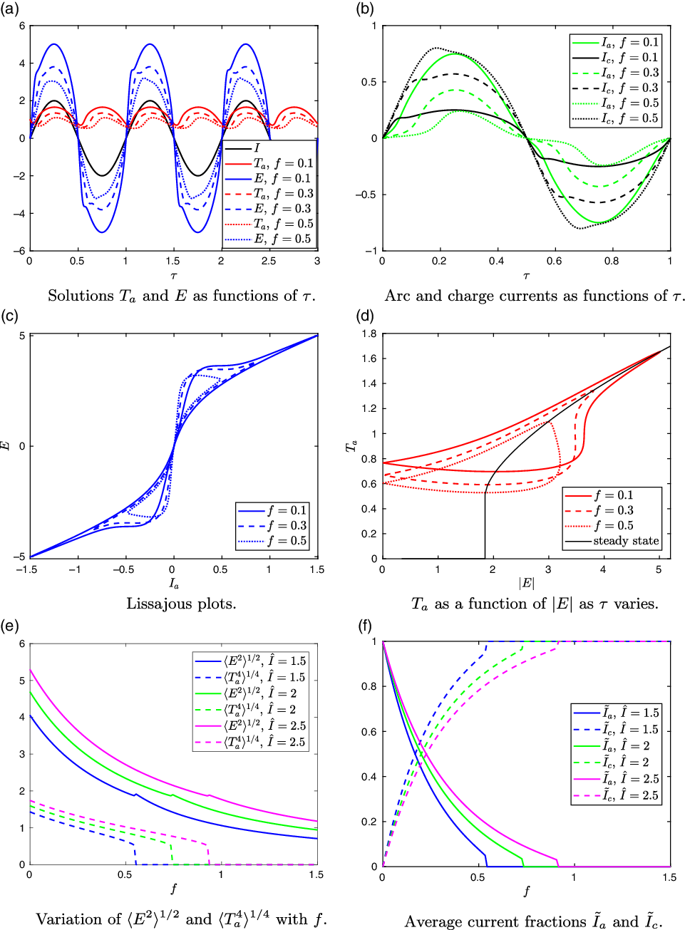


The arc temperature
 $T_a$
in Figure 2(a) oscillates over the AC cycle, with period half of the AC period. There is a time delay in this process, so that the arc temperature minimum occurs after the current passes through zero. For larger values of f, less current passes through the arc, so that the temperature
$T_a$
in Figure 2(a) oscillates over the AC cycle, with period half of the AC period. There is a time delay in this process, so that the arc temperature minimum occurs after the current passes through zero. For larger values of f, less current passes through the arc, so that the temperature
 $T_a$
is lower. The time delay of the arc temperature is more pronounced for larger f, and the asymmetry is visible: there is a faster increase in temperature as the arc ignites and a slower decay as the current passes through zero.
$T_a$
is lower. The time delay of the arc temperature is more pronounced for larger f, and the asymmetry is visible: there is a faster increase in temperature as the arc ignites and a slower decay as the current passes through zero.
Lissajous plots (showing electric field E against arc current
 $I_a$
) corresponding to the solutions in Figure 2(a) are shown in Figure 2(c). Industrially, these Lissajous plots are known as the ‘arc signature’ and are used to visualise the electrical conditions in the furnace. An example arc signature, computed from measurements from an operational furnace, and the expected shape of the arc signature according to [Reference Valderhaug52] are shown in Figure 3.
$I_a$
) corresponding to the solutions in Figure 2(a) are shown in Figure 2(c). Industrially, these Lissajous plots are known as the ‘arc signature’ and are used to visualise the electrical conditions in the furnace. An example arc signature, computed from measurements from an operational furnace, and the expected shape of the arc signature according to [Reference Valderhaug52] are shown in Figure 3.

Figure 3. Lissajous plots (arc voltage against arc current) in the SAF literature. Left: an example arc signature computed from measurements of an operational silicon furnace [24]. Right: an illustration of the expected shape of the arc signature, reproduced from [Reference Valderhaug52] (Figure 3.23, p. 94).
Our simulated Lissajous plots in Figure 2(c) bear reasonable qualitative similarity to the arc signatures in Figure 3, and also to those elsewhere in the literature [Reference Sævarsdóttir39, Reference Schei, Tuset and Tveit42]. The large-f curve in Figure 2(c) is most similar to that on the left of Figure 3, and the smaller f curves are similar to that on the right of Figure 3, although we find the ‘points’ of the curve angle upwards, unlike the horizontal points anticipated on the right of Figure 3. The cause of the different shapes may be understood by considering the changing temperature of the arc over the AC cycle. In Figure 2(d),
 $T_a$
is plotted against the magnitude of the electric field
$T_a$
is plotted against the magnitude of the electric field
 $|E|$
for various f. In Figure 2(d), we also plot, in black, the steady-state solution of the arc temperature equation, i.e., of
$|E|$
for various f. In Figure 2(d), we also plot, in black, the steady-state solution of the arc temperature equation, i.e., of
 $T_a^4=E^2\sigma_a(T_a)$
, which we might interpret as the arc temperature for a much more slowly varying electric current, or the direct current (DC) solution. We note that there are in fact three steady-state solutions
$T_a^4=E^2\sigma_a(T_a)$
, which we might interpret as the arc temperature for a much more slowly varying electric current, or the direct current (DC) solution. We note that there are in fact three steady-state solutions
 $T_a$
for large enough E; here, we show the nontrivial, stable solution where this exists. We observe that the
$T_a$
for large enough E; here, we show the nontrivial, stable solution where this exists. We observe that the
 $\tau$
-varying curves pass through the steady-state curve at the maximum electric field. For smaller f, when a greater proportion of the current passes through the arc, the
$\tau$
-varying curves pass through the steady-state curve at the maximum electric field. For smaller f, when a greater proportion of the current passes through the arc, the
 $\tau$
-varying curve more closely follows the steady-state curve. It is this behaviour that may also be seen in the variety of Lissajous shapes in Figure 2(c). One could therefore use the shape of the Lissajous plots for operational furnaces to interpret how much current is passing through the arc: assuming the total applied current amplitude is constant, rounder shapes suggest more current is passing through the charge material. For instance, one might infer that a reasonable proportion of the current is passing through the charge material in the left of Figure 3, whereas the majority of the current is through the arc on the right of Figure 3.
$\tau$
-varying curve more closely follows the steady-state curve. It is this behaviour that may also be seen in the variety of Lissajous shapes in Figure 2(c). One could therefore use the shape of the Lissajous plots for operational furnaces to interpret how much current is passing through the arc: assuming the total applied current amplitude is constant, rounder shapes suggest more current is passing through the charge material. For instance, one might infer that a reasonable proportion of the current is passing through the charge material in the left of Figure 3, whereas the majority of the current is through the arc on the right of Figure 3.
From these
 $\tau$
-varying solutions, we may compute the averaged quantities
$\tau$
-varying solutions, we may compute the averaged quantities
 $\langle E^2\rangle$
and
$\langle E^2\rangle$
and
 $\langle T_a^4\rangle$
needed for the homogenised problem (3.18c)–(3.18l) in the charge material, by averaging the periodic solutions over the AC period. For a given applied current amplitude
$\langle T_a^4\rangle$
needed for the homogenised problem (3.18c)–(3.18l) in the charge material, by averaging the periodic solutions over the AC period. For a given applied current amplitude
 $\hat{I}$
, we may compute these averaged quantities
$\hat{I}$
, we may compute these averaged quantities
 $\langle E^2\rangle^{1/2}$
and
$\langle E^2\rangle^{1/2}$
and
 $\langle T_a^4\rangle^{1/4}$
for a range of values of f, as shown in Figure 2(e). We note from Figure 2(d) that below a critical electrical field,
$\langle T_a^4\rangle^{1/4}$
for a range of values of f, as shown in Figure 2(e). We note from Figure 2(d) that below a critical electrical field,
 $\langle E^2\rangle^{1/2}_{\text{crit}}$
, there is no non-trivial DC or steady-state solution of the arc temperature equation (for
$\langle E^2\rangle^{1/2}_{\text{crit}}$
, there is no non-trivial DC or steady-state solution of the arc temperature equation (for
 $\hat{I}=2$
as in Figure 2(d), this critical value is
$\hat{I}=2$
as in Figure 2(d), this critical value is
 $\langle E^2\rangle^{1/2}_{\text{crit}}\approx 1.85$
). Below this same
$\langle E^2\rangle^{1/2}_{\text{crit}}\approx 1.85$
). Below this same
 $\langle E^2\rangle^{1/2}_{\text{crit}}$
we see in Figure 2(e) that
$\langle E^2\rangle^{1/2}_{\text{crit}}$
we see in Figure 2(e) that
 $\langle T_a^4\rangle=0$
and that there is therefore no arc in the AC case either. In Figure 2(f), we show the fraction of the average of the magnitude of the currents passing through the arc and charge material, respectively, namely
$\langle T_a^4\rangle=0$
and that there is therefore no arc in the AC case either. In Figure 2(f), we show the fraction of the average of the magnitude of the currents passing through the arc and charge material, respectively, namely
 $\tilde{I}_a:=\pi\langle |\sigma_a(T_a)E|\rangle/(2\hat{I})$
and
$\tilde{I}_a:=\pi\langle |\sigma_a(T_a)E|\rangle/(2\hat{I})$
and
 $\tilde{I}_c:=\pi f\langle |E|\rangle/(2\hat{I}),$
where the average of the magnitude of the total current is
$\tilde{I}_c:=\pi f\langle |E|\rangle/(2\hat{I}),$
where the average of the magnitude of the total current is
 $\langle |I|\rangle=2\hat{I}/\pi$
, so that we do indeed have
$\langle |I|\rangle=2\hat{I}/\pi$
, so that we do indeed have
 $\tilde{I}_a+\tilde{I}_c=1$
. We observe that
$\tilde{I}_a+\tilde{I}_c=1$
. We observe that
 $\tilde{I}_a$
decreases with f, as more current flows instead through the charge material. We also note that for each
$\tilde{I}_a$
decreases with f, as more current flows instead through the charge material. We also note that for each
 $\hat{I}$
there is a critical value of f above which
$\hat{I}$
there is a critical value of f above which
 $\langle E^2\rangle^{1/2}<\langle E^2\rangle^{1/2}_{\text{crit}}$
and the average arc temperature
$\langle E^2\rangle^{1/2}<\langle E^2\rangle^{1/2}_{\text{crit}}$
and the average arc temperature
 $\langle T_a^4\rangle$
becomes zero, so that in Figure 2(f) we have
$\langle T_a^4\rangle$
becomes zero, so that in Figure 2(f) we have
 $\tilde{I}_a=0,$
and
$\tilde{I}_a=0,$
and
 $\tilde{I}_c=1$
, and all current passes through the charge.
$\tilde{I}_c=1$
, and all current passes through the charge.
Compared with many arc models in the literature, (3.18a) is fairly simple, but neverthless it appears to capture much of the qualitative alternating current behaviour of the electrical system seen in practice, including the figure-of-eight shaped Lissajous plots in Figure 2(c). However, our model does not exhibit the phase shift expected in practice between the current and electric field created by the three-phase current, explored in [Reference Valderhaug52]. Neither does it incorporate any asymmetry in the two half-periods when first the electrode and then the crater boundary or melt-pool act as cathode. We do not explore these additional points here.
4.2 Solutions of the coupled model
We first note that the problem for the gas variables
 $u_g, C_g$
and
$u_g, C_g$
and
 $T_g$
decouples from that of the solid variables. Given the solution of the solid problem, we may compute the gas variables as follows. Adding (3.18c) and (3.18d), and integrating the resulting expression using (3.18j)–(3.18k), we express the gas flux as a sum of the flux through the free boundary at
$T_g$
decouples from that of the solid variables. Given the solution of the solid problem, we may compute the gas variables as follows. Adding (3.18c) and (3.18d), and integrating the resulting expression using (3.18j)–(3.18k), we express the gas flux as a sum of the flux through the free boundary at
 $r=s(t)$
, and the material produced by reaction in the charge material:
$r=s(t)$
, and the material produced by reaction in the charge material:
 \begin{equation}u_gC_g=\left(\frac{1}{s}+\dot{s}\right)\left(C_s-C_*\right)+R_ps.\end{equation}
Integrating (3.18g) and substituting (4.1) for
 $u_gC_g$
, we obtain
$u_gC_g$
, we obtain
 \begin{equation}T_g=\frac{R_psT_s(0)+\int_0^XT_s\mathcal{Q}\,\textrm{d}\hat{X}}{R_ps+\left(\dot{s}+\frac{1}{s}\right)(C_s-C_*)}.\end{equation}
Finally, using (3.18e) and (4.1) we find
 \begin{align}C_g&=\frac{(1-C_s)(R_ps+\left(\dot{s}+\frac{1}{s}\right)(C_s-C_*))}{R_psT_s(0)+\int_0^XT_s\mathcal{Q}\,\textrm{d}\hat{X}}, & u_g&=\frac{R_psT_s(0)+\int_0^XT_s\mathcal{Q}\,\textrm{d}\hat{X}}{1-C_s},\end{align}
and so may compute the gas variables once the solution of the coupled arc and solid charge problem is known.
We solve numerically the quasi-steady system (3.18) for a given constant applied current amplitude
 $\hat{I}$
. To do this, we first solve the arc problem (3.18a) as described in Section 4.1, for a range of values of f, computing a look-up table for the values of
$\hat{I}$
. To do this, we first solve the arc problem (3.18a) as described in Section 4.1, for a range of values of f, computing a look-up table for the values of
 $\langle T_a^4\rangle$
and
$\langle T_a^4\rangle$
and
 $\langle E^2\rangle$
as functions of f. Prescribing the value of s, we then solve the boundary value problem in the charge material for
$\langle E^2\rangle$
as functions of f. Prescribing the value of s, we then solve the boundary value problem in the charge material for
 $C_s$
and
$C_s$
and
 $T_s$
, simultaneously solving for
$T_s$
, simultaneously solving for
 $\dot{s}$
,
$\dot{s}$
,
 $\langle E^2\rangle,$
and
$\langle E^2\rangle,$
and
 $\langle T_a^4\rangle$
using the look-up table. We impose the integral constraint in (3.18a) by converting it to an extra differential equation, which gives the boundary value problem
$\langle T_a^4\rangle$
using the look-up table. We impose the integral constraint in (3.18a) by converting it to an extra differential equation, which gives the boundary value problem
 \begin{align} Z(X)&=\alpha s\int_0^X\sigma_c (\hat{X})\,\textrm{d}\hat{X}, & Z'(X)&=\alpha s\sigma_c(X), & Z(0)&=0, & Z(\infty)=f.\end{align}
The far-field behaviour
 $T_s\rightarrow T_s^\infty$
is imposed using the mixed condition
$T_s\rightarrow T_s^\infty$
is imposed using the mixed condition
 \begin{equation}{\frac{\partial{T_s}}{\partial{X}}}+\left(\frac{1}{s}+\dot{s}\right)C_s^\infty(T_s-T_s^\infty)\rightarrow 0 \quad \text{as}\quad X \rightarrow \infty,\end{equation}
which may be derived from (3.18f) and (3.18l) and reduces the required domain size. The numerical solutions are computed using the MATLAB in-built solver bvp4c, which uses a Runge-Kutta finite-difference formula and collocation method to choose and refine the mesh [Reference Kierzenka and Shampine28]. By varying the prescribed value of s, we sweep through the time-dependence of the solutions.
Solutions for various
 $\hat{I}$
are summarised in Figure 4. We see that for large enough values of
$\hat{I}$
are summarised in Figure 4. We see that for large enough values of
 $\hat{I}$
, greater than a critical value
$\hat{I}$
, greater than a critical value
 $\hat{I}_{\text{crit}}\approx 1.8$
as in Figure 4(a), there are two steady state solutions, which we refer to as
$\hat{I}_{\text{crit}}\approx 1.8$
as in Figure 4(a), there are two steady state solutions, which we refer to as
 $s=s_1$
and
$s=s_1$
and
 $s=s_2>s_1$
, respectively, whereas for
$s=s_2>s_1$
, respectively, whereas for
 $\hat{I}<\hat{I}_{\text{crit}}$
, we have not been able to find any steady-state solutions. In Figure 4(b), we show the variation of
$\hat{I}<\hat{I}_{\text{crit}}$
, we have not been able to find any steady-state solutions. In Figure 4(b), we show the variation of
 $\dot{s}$
with s for various values of
$\dot{s}$
with s for various values of
 $\hat{I}$
. For small
$\hat{I}$
. For small
 $\hat{I}<\hat{I}_{\text{crit}}$
, we see that
$\hat{I}<\hat{I}_{\text{crit}}$
, we see that
 $\dot{s}<0$
for all s, so that the crater collapses: there is insufficient energy for the chemical reactions to consume the incoming material. For
$\dot{s}<0$
for all s, so that the crater collapses: there is insufficient energy for the chemical reactions to consume the incoming material. For
 $\hat{I}>\hat{I}_{\text{crit}}$
, we see that
$\hat{I}>\hat{I}_{\text{crit}}$
, we see that
 \begin{align}\dot{s}<0 \quad \text{ if } s<s_1 \text{ or }s>s_2, \qquad \text{ and } \qquad \dot{s}>0 \quad \text{ if } s\in (s_1,s_2),\end{align}
so that all solutions evolve towards
 $s_2$
unless initially
$s_2$
unless initially
 $s<s_1$
. For
$s<s_1$
. For
 $s>s_2$
, the solutions all initiate near the curve
$s>s_2$
, the solutions all initiate near the curve
 $\dot{s}=-1/s$
, which corresponds to the crater wall
$\dot{s}=-1/s$
, which corresponds to the crater wall
 $r=s$
moving inward at the same speed,
$r=s$
moving inward at the same speed,
 $-1/s$
, as the inflowing solid material: at this value of s, the solid material is too cold for the chemical reactions take place. As we increase
$-1/s$
, as the inflowing solid material: at this value of s, the solid material is too cold for the chemical reactions take place. As we increase
 $\hat{I}$
, the stable steady state
$\hat{I}$
, the stable steady state
 $s=s_2$
increases, so that we expect larger craters in furnaces with higher currents. We discuss the structure and evolution of these solutions further in Section 4.3, in terms of the overall balance of energy in the system.
$s=s_2$
increases, so that we expect larger craters in furnaces with higher currents. We discuss the structure and evolution of these solutions further in Section 4.3, in terms of the overall balance of energy in the system.

Figure 4. Numerical solutions of the model (3.18) using the typical parameter values in Table 3, with
 $C_*=0.2,$
 $C_s^\infty=0.75$
and
$C_s^\infty=0.75$
and
 $T_s^\infty=0.33$
.
$T_s^\infty=0.33$
.
The temperature profiles
 $T_s(X)$
and
$T_s(X)$
and
 $T_g(X)$
are shown in Figure 4(c), and the concentration profiles
$T_g(X)$
are shown in Figure 4(c), and the concentration profiles
 $C_s$
and
$C_s$
and
 $C_g$
are shown in Figure 4(d), in both cases at various points along the
$C_g$
are shown in Figure 4(d), in both cases at various points along the
 $\hat{I}=2$
solution, marked with crosses in Figure 4(b). The solid temperature
$\hat{I}=2$
solution, marked with crosses in Figure 4(b). The solid temperature
 $T_s$
decreases monotonically from its maximum at
$T_s$
decreases monotonically from its maximum at
 $X=0$
to the far-field
$X=0$
to the far-field
 $T_s^\infty$
. The solid concentration
$T_s^\infty$
. The solid concentration
 $C_s$
increases from
$C_s$
increases from
 $C_*$
at
$C_*$
at
 $X=0$
to the far-field value
$X=0$
to the far-field value
 $C_s^\infty$
by the point
$C_s^\infty$
by the point
 $T_s=T_m$
, whereafter
$T_s=T_m$
, whereafter
 $\mathcal{Q}=0$
. The gas is likewise hottest as it leaves the crater at
$\mathcal{Q}=0$
. The gas is likewise hottest as it leaves the crater at
 $X=0$
, cooling due to the production of gas, despite the heat,
$X=0$
, cooling due to the production of gas, despite the heat,
 $T_s\mathcal{Q}$
, that this newly formed gas brings with it. The gas temperature reaches a constant value,
$T_s\mathcal{Q}$
, that this newly formed gas brings with it. The gas temperature reaches a constant value,
 $T_g^\infty$
say, by the point
$T_g^\infty$
say, by the point
 $T_s=T_m$
, whereafter
$T_s=T_m$
, whereafter
 $\mathcal{Q}=0$
and both
$\mathcal{Q}=0$
and both
 $C_s$
and
$C_s$
and
 $C_g$
are constant. The concentration
$C_g$
are constant. The concentration
 $C_g$
of the gas, given by (4.3), decreases with X from a maximum at
$C_g$
of the gas, given by (4.3), decreases with X from a maximum at
 $X=0$
, due to the decreasing porosity of the charge material as
$X=0$
, due to the decreasing porosity of the charge material as
 $C_s$
increases. Since the gas flux
$C_s$
increases. Since the gas flux
 $u_gC_g$
increases linearly with
$u_gC_g$
increases linearly with
 $C_s$
according to (4.1), and since
$C_s$
according to (4.1), and since
 $C_s$
increases with X, the gas velocity,
$C_s$
increases with X, the gas velocity,
 $u_g$
, behaving like
$u_g$
, behaving like
 $C_s/C_g$
, must also increase with X until the point
$C_s/C_g$
, must also increase with X until the point
 $T_s=T_m$
.
$T_s=T_m$
.
As s decreases, we see from Figure 4(c) that the temperature at the crater wall
 $X=0$
increases dramatically, as the heat radiated by the arc is distributed over a smaller surface area. The rate of decay of
$X=0$
increases dramatically, as the heat radiated by the arc is distributed over a smaller surface area. The rate of decay of
 $T_s$
with X is also faster for smaller s, so that the region of X for which
$T_s$
with X is also faster for smaller s, so that the region of X for which
 $\mathcal{Q}>0$
and
$\mathcal{Q}>0$
and
 $T_g,C_s$
and
$T_g,C_s$
and
 $C_g$
vary, is narrower.
$C_g$
vary, is narrower.
4.3 Overall power balance
We can understand the structure of the solutions found in the previous section by considering the overall balance of power in the system.
Adding the equations for conservation of energy in the gas and in the solid, (3.18g) and (3.18f), the terms modelling the heat transfer between the solid and gas cancel, and, making use of the form (4.1) of
 $u_gC_g$
, we obtain
$u_gC_g$
, we obtain
 \begin{equation}{\frac{\partial{ }}{\partial{X}}}\bigg[ \left(\left(\frac{1}{s}+\dot{s}\right)(C_s-C_*)+R_ps\right)T_g-\left(\frac{1}{s}+\dot{s}\right)C_s(T_s-\gamma)-{\frac{\partial{T_s}}{\partial{X}}}\bigg]=\alpha\sigma_c\langle E^2\rangle,\end{equation}
where we have also used (3.18c) to write the heat lost to chemical reaction as a derivative of
 $C_s$
. Integrating over the entire charge domain
$C_s$
. Integrating over the entire charge domain
 $X\in[0,\infty)$
and applying the boundary conditions (3.18h)–(3.18l), we obtain a total energy balance of the system, namely
$X\in[0,\infty)$
and applying the boundary conditions (3.18h)–(3.18l), we obtain a total energy balance of the system, namely
 \begin{equation}\begin{aligned}\langle EI\rangle & = \gamma\left(\left(1+s\dot{s}\right)(C_s^\infty-C_*)+s^2R_p\right) +s^2\kappa^*(T_s(0)-T_s^\infty)-(1+s\dot{s})C_s^\infty T_s^\infty\\[3pt]&\qquad +\left((1+s\dot{s})(C_s^\infty-C_*)+R_ps^2\right)T_g^\infty.\end{aligned}\end{equation}
On the left of (4.8), we have the total electrical energy dissipated in the system per unit time over both the arc and the charge which, by averaging the fast-timescale equations (3.18a), is given by
 \begin{equation}\langle EI\rangle=\langle T_a^4\rangle+\alpha s\langle E^2\rangle\int_0^\infty\sigma_c\,\textrm{d}X.\end{equation}
The terms on the right of (4.8) are, respectively, power consumed by chemical reactions, both in the charge and in the melt-pool, power lost by conduction through the top and base of the crater, power gained in the warm incoming solid charge material, and power lost in the flow of hot gases out at infinity. The gas temperature at infinity,
 $T_g^\infty$
, is determined as part of the solution. The unknowns in (4.8) are therefore
$T_g^\infty$
, is determined as part of the solution. The unknowns in (4.8) are therefore
 $E, s, \dot{s}, T_s(0)$
and
$E, s, \dot{s}, T_s(0)$
and
 $T_g^\infty$
. We may consider these to be functions of the position of the free boundary s rather than of time t, since (numerically) we have found a single solution, and so a single value of
$T_g^\infty$
. We may consider these to be functions of the position of the free boundary s rather than of time t, since (numerically) we have found a single solution, and so a single value of
 $E, \dot{s}, T_s(0)$
and
$E, \dot{s}, T_s(0)$
and
 $T_g^\infty$
, for each value s.
$T_g^\infty$
, for each value s.
Rearranging (4.8), we find
 \begin{equation}s\dot{s}=\frac{\langle EI\rangle -H_R}{H_R}-\frac{H_V}{H_R}s^2,\end{equation}
where
 $H_R=(\gamma+T_g^\infty)(C_s^\infty-C_*)-C_s^\infty T_s^\infty$
and
$H_R=(\gamma+T_g^\infty)(C_s^\infty-C_*)-C_s^\infty T_s^\infty$
and
 $H_V=\kappa^*(T_s(0)-T_s^\infty)+R_p(\gamma+T_g^\infty),$
are, respectively, the heat losses in the radial direction (the heat lost to chemical reaction in the charge material, the heat gained from incoming charge material at infinity and the heat lost in the hot gas that escapes to infinity) and the heat losses per unit area in the vertical direction (chemical and conductive heat losses in the melt pool at the base of the cylindrical crater, and through the electrode at the top). We assume that both
$H_V=\kappa^*(T_s(0)-T_s^\infty)+R_p(\gamma+T_g^\infty),$
are, respectively, the heat losses in the radial direction (the heat lost to chemical reaction in the charge material, the heat gained from incoming charge material at infinity and the heat lost in the hot gas that escapes to infinity) and the heat losses per unit area in the vertical direction (chemical and conductive heat losses in the melt pool at the base of the cylindrical crater, and through the electrode at the top). We assume that both
 $H_R$
and
$H_R$
and
 $H_V$
are positive, i.e., that
$H_V$
are positive, i.e., that
 $C_s^\infty T_s^\infty$
is sufficiently small and that
$C_s^\infty T_s^\infty$
is sufficiently small and that
 $T_s(0)\geq T_s^\infty$
.
$T_s(0)\geq T_s^\infty$
.
In order for a steady-state solution, with
 $\dot{s}=0$
, to exist, we see from (4.10) that we require
$\dot{s}=0$
, to exist, we see from (4.10) that we require
 $\langle EI\rangle-H_R>0$
, and hence we need a sufficiently high electrical power
$\langle EI\rangle-H_R>0$
, and hence we need a sufficiently high electrical power
 $\langle EI\rangle $
. If the electrical power is too low, then the first term of (4.10) is negative, or small and positive, and so
$\langle EI\rangle $
. If the electrical power is too low, then the first term of (4.10) is negative, or small and positive, and so
 $\dot{s}<0$
for all s. In this case, the crater will collapse inward, as the electrical power dissipated will be insufficient to react away the incoming flux of solid material. This is the behaviour observed for the numerical solutions in Section 4.2, when the applied current had too small an amplitude
$\dot{s}<0$
for all s. In this case, the crater will collapse inward, as the electrical power dissipated will be insufficient to react away the incoming flux of solid material. This is the behaviour observed for the numerical solutions in Section 4.2, when the applied current had too small an amplitude
 $\hat{I}<\hat{I}_{\text{crit}}$
.
$\hat{I}<\hat{I}_{\text{crit}}$
.
If the applied current is sufficiently large that solutions
 $\langle EI\rangle -H_R>0$
exist, then we expect there to be steady-state solutions. In Figure 5(a), we show the variation of
$\langle EI\rangle -H_R>0$
exist, then we expect there to be steady-state solutions. In Figure 5(a), we show the variation of
 $T_s(0),T_g^\infty$
and
$T_s(0),T_g^\infty$
and
 $\langle EI\rangle$
with s, from the numerical solutions computed in Section 4.2. For large enough s, all three of
$\langle EI\rangle$
with s, from the numerical solutions computed in Section 4.2. For large enough s, all three of
 $T_s(0),T_g^\infty$
and
$T_s(0),T_g^\infty$
and
 $\langle EI\rangle$
vary slowly with s, so that for large enough s,
$\langle EI\rangle$
vary slowly with s, so that for large enough s,
 $\langle EI\rangle, H_R$
and
$\langle EI\rangle, H_R$
and
 $H_V$
are approximately constants. Therefore, if there is a steady- state solution
$H_V$
are approximately constants. Therefore, if there is a steady- state solution
 $s^*$
in this range of sufficiently large s, then from (4.10), we see that for
$s^*$
in this range of sufficiently large s, then from (4.10), we see that for
 $s>s^*$
, we have
$s>s^*$
, we have
 $\dot{s}<0$
, while for
$\dot{s}<0$
, while for
 $s<s^*$
, we have
$s<s^*$
, we have
 $\dot{s}>0$
. Thus, such a steady state is stable. This describes the behaviour of the larger steady state
$\dot{s}>0$
. Thus, such a steady state is stable. This describes the behaviour of the larger steady state
 $s=s_2$
seen numerically in Section 4.2. We note that it is the changing geometry of the system that determines the stability of this steady state: since
$s=s_2$
seen numerically in Section 4.2. We note that it is the changing geometry of the system that determines the stability of this steady state: since
 $H_R,H_V$
and
$H_R,H_V$
and
 $\langle EI\rangle$
are all approximately constant, the increasing surface area of the crater top and base, which behaves like
$\langle EI\rangle$
are all approximately constant, the increasing surface area of the crater top and base, which behaves like
 $s^2$
, means that as s increases from
$s^2$
, means that as s increases from
 $s_2$
the heat loss in the vertical direction increases while the total energy produced does not vary much, and hence
$s_2$
the heat loss in the vertical direction increases while the total energy produced does not vary much, and hence
 $\dot{s}$
decreases through the steady state, making it stable.
$\dot{s}$
decreases through the steady state, making it stable.

Figure 5. Behaviour of
 $\langle EI\rangle$
,
$\langle EI\rangle$
,
 $T_s(0)$
,
$T_s(0)$
,
 $T_g^\infty$
with s, corresponding to the numerical solutions presented in Figure 4.
$T_g^\infty$
with s, corresponding to the numerical solutions presented in Figure 4.
From Figure 5(a), we see that as s becomes small, while
 $\langle EI\rangle$
remains roughly constant,
$\langle EI\rangle$
remains roughly constant,
 $T_s(0)$
and
$T_s(0)$
and
 $T_g^\infty$
increase dramatically. This is because the energy radiated from the arc remains roughly constant, but is distributed over an increasingly small surface area, causing
$T_g^\infty$
increase dramatically. This is because the energy radiated from the arc remains roughly constant, but is distributed over an increasingly small surface area, causing
 $T_s(0)$
to blow up, which causes a similar, but lesser, increase in
$T_s(0)$
to blow up, which causes a similar, but lesser, increase in
 $T_g^\infty$
. Since both
$T_g^\infty$
. Since both
 $H_V$
and
$H_V$
and
 $H_R$
are linear in
$H_R$
are linear in
 $T_g^\infty$
or
$T_g^\infty$
or
 $T_s(0)$
, these blow up as s becomes small, causing
$T_s(0)$
, these blow up as s becomes small, causing
 $\dot{s}$
to become negative for small s. This is the cause of the second steady state,
$\dot{s}$
to become negative for small s. This is the cause of the second steady state,
 $s_1$
, observed numerically. Specifically, from the numerical solutions in Figure 5(b) we see that, even though
$s_1$
, observed numerically. Specifically, from the numerical solutions in Figure 5(b) we see that, even though
 $T_s(0)$
increases faster than
$T_s(0)$
increases faster than
 $T_g^\infty$
as s becomes small,
$T_g^\infty$
as s becomes small,
 $(T_s(0)/T_g^\infty)s^2$
is bounded, and approaches zero as
$(T_s(0)/T_g^\infty)s^2$
is bounded, and approaches zero as
 $s\rightarrow 0$
. Thus, the quadratic-type term,
$s\rightarrow 0$
. Thus, the quadratic-type term,
 $(H_V/H_R)s^2$
, in (4.10) remains bounded. The change in the sign of
$(H_V/H_R)s^2$
, in (4.10) remains bounded. The change in the sign of
 $\dot{s}$
as s becomes small is therefore due to the change in sign of the first term, or of
$\dot{s}$
as s becomes small is therefore due to the change in sign of the first term, or of
 $\langle EI\rangle-H_R$
. Thus, it is the blow-up in the heat,
$\langle EI\rangle-H_R$
. Thus, it is the blow-up in the heat,
 $T_g^\infty(C_s^\infty-C_*)$
, lost in the gas escaping at infinity that creates the second steady state
$T_g^\infty(C_s^\infty-C_*)$
, lost in the gas escaping at infinity that creates the second steady state
 $s_1$
.
$s_1$
.
4.4 Crater evolution and the stoking of industrial furnaces
We have seen that when
 $\hat{I}$
is large enough for steady states
$\hat{I}$
is large enough for steady states
 $s_1$
and
$s_1$
and
 $s_2$
to exist, the system evolves from any initial state with
$s_2$
to exist, the system evolves from any initial state with
 $s>s_1$
to the larger steady state
$s>s_1$
to the larger steady state
 $s_2$
over the timescale
$s_2$
over the timescale
 $[t_s]\approx 5$
h as in Section 2.6. However, the steady state
$[t_s]\approx 5$
h as in Section 2.6. However, the steady state
 $s_2$
is unlikely to be attained in reality, due to the practice of stoking.
$s_2$
is unlikely to be attained in reality, due to the practice of stoking.
In realistic industrial configurations, the furnace is stoked at regular intervals (on the order of 45 min to an hour). The stoking process involves manually breaking up and mixing the top layer of charge material in the furnace, using a large pole (in the same way one might stoke a fire with a poker). This practice ensures the gases can flow out through the charge, preventing gas blows and ensuring good silicon production. Stoking is also seen to increase the flow of solid material down towards the crater, and it is understood that during stoking the crater quickly shrinks, before slowly growing back outwards until the next stoking.
While our model is not designed to capture rapid changes in the flux of solid material to the crater, we can understand the stoking cycle in terms of an instantaneous re-setting of the crater radius s during the stoking. Since the dimensional analysis suggests that the temperature and concentration fields are all quasi-steady on the
 $[t_s]$
timescale, we expect to rapidly revert to the quasi-steady
$[t_s]$
timescale, we expect to rapidly revert to the quasi-steady
 $\dot{s}(s)$
solution curve. Stoking can therefore be thought of as rapidly reducing the crater radius to a smaller value of s, and the system instantaneously reverting to the
$\dot{s}(s)$
solution curve. Stoking can therefore be thought of as rapidly reducing the crater radius to a smaller value of s, and the system instantaneously reverting to the
 $\dot{s}(s)$
solution curve for the new value of s. The system then evolves slowly along the
$\dot{s}(s)$
solution curve for the new value of s. The system then evolves slowly along the
 $\dot{s}(s)$
curve, with s increasing towards
$\dot{s}(s)$
curve, with s increasing towards
 $s_2$
until the next stoking period. The current distribution through the furnace varies as we pass along the curve. Immediately after stoking, we would expect the fraction of the current passing through the charge to be greater and then to decrease steadily again as s increases.
$s_2$
until the next stoking period. The current distribution through the furnace varies as we pass along the curve. Immediately after stoking, we would expect the fraction of the current passing through the charge to be greater and then to decrease steadily again as s increases.
Within this framework, we can also understand the effect of stoking on the overall reaction rate. We consider the total chemical reaction, defined by
 \begin{equation} \mathcal{Q}_T=s\int_{X=0}^\infty \mathcal{Q} \,\textrm{d}X,\end{equation}
which, if redimensionalised, would have dimensions
 $[\textrm{mol}\,\textrm{s}^{-1}]$
. Since this is the rate at which charge material is consumed, we may think of it as a proxy for the silicon production rate. We note that, in reality, the silicon production rate is not necessarily equal to the rate of production of SiO gas, since some SiO gas may be lost out of the top surface of the charge material, and so is not converted to silicon.
$[\textrm{mol}\,\textrm{s}^{-1}]$
. Since this is the rate at which charge material is consumed, we may think of it as a proxy for the silicon production rate. We note that, in reality, the silicon production rate is not necessarily equal to the rate of production of SiO gas, since some SiO gas may be lost out of the top surface of the charge material, and so is not converted to silicon.
By integrating the equation of conservation of mass (3.18c), we see that
 \begin{equation} \mathcal{Q}_T=s\int_{X=0}^\infty \left(\dot{s}+\frac{1}{s}\right){\frac{\partial{C_s}}{\partial{X}}} \, \textrm{d}X=(1+s\dot{s})(C_s^\infty-C_*).\end{equation}
While this expression has no explicit dependence on the functional form of
 $\mathcal{Q}$
, we note that the dependence is through the values of s and
$\mathcal{Q}$
, we note that the dependence is through the values of s and
 $\dot{s}$
in the solution.
$\dot{s}$
in the solution.
Taking partial derivatives of (4.12) with respect to s we see that
 \begin{equation} {\frac{\partial{\mathcal{Q}_T}}{\partial{s}}}=(C_s^\infty-C_*)\left(\dot{s}+s{\frac{\partial{\dot{s}}}{\partial{s}}}\right).\end{equation}
We suppose that the furnace is running at sufficiently high current that steady states of our model exist:
 $s=s_1$
and
$s=s_1$
and
 $s=s_2>s_1$
. At each of these steady states,
$s=s_2>s_1$
. At each of these steady states,
 $\mathcal{Q}_T=C_s^\infty-C_*$
, and further, since
$\mathcal{Q}_T=C_s^\infty-C_*$
, and further, since
 ${\frac{\partial{\dot{s}}}{\partial{s}}}>0 \text{ at }s=s_1,$
and
${\frac{\partial{\dot{s}}}{\partial{s}}}>0 \text{ at }s=s_1,$
and
 ${\frac{\partial{\dot{s}}}{\partial{s}}}<0 \text{ at }s=s_2,$
we see that
${\frac{\partial{\dot{s}}}{\partial{s}}}<0 \text{ at }s=s_2,$
we see that
 \begin{align}{\frac{\partial{\mathcal{Q}_T}}{\partial{s}}}>0 \text{ at }s=s_1 \quad \text{and} \quad {\frac{\partial{\mathcal{Q}_T}}{\partial{s}}}<0 \text{ at }s=s_2.\end{align}
Hence, the maximum value of
 $\mathcal{Q}_T$
must always be between
$\mathcal{Q}_T$
must always be between
 $s_1$
and
$s_1$
and
 $s_2$
. This is illustrated in Figure 6 (left), in which we show the variation of
$s_2$
. This is illustrated in Figure 6 (left), in which we show the variation of
 $\mathcal{Q}_T$
with s along solution curves
$\mathcal{Q}_T$
with s along solution curves
 $\dot{s}(s)$
.
$\dot{s}(s)$
.

Figure 6. Behaviour of total reaction rate
 $\mathcal{Q}_T$
corresponding to the numerical solutions presented in Figure 4: variation of
$\mathcal{Q}_T$
corresponding to the numerical solutions presented in Figure 4: variation of
 $\mathcal{Q}_T$
with s for various
$\mathcal{Q}_T$
with s for various
 $\hat{I}$
, with the dotted line showing the value of
$\hat{I}$
, with the dotted line showing the value of
 $\mathcal{Q}_T=C_s^\infty-C_*$
at the steady states
$\mathcal{Q}_T=C_s^\infty-C_*$
at the steady states
 $s=s_1$
and
$s=s_1$
and
 $s_2$
(left), and the maximum over s of
$s_2$
(left), and the maximum over s of
 $\mathcal{Q}_T$
, as
$\mathcal{Q}_T$
, as
 $\hat{I}$
varies (right).
$\hat{I}$
varies (right).
By stoking the furnace, and so repeatedly pushing s below
 $s_2$
, we must increase
$s_2$
, we must increase
 $\mathcal{Q}_T$
. Thus, by integrating
$\mathcal{Q}_T$
. Thus, by integrating
 $\mathcal{Q}_T$
over the time of many stoking cycles, we see that the overall rate of consumption of solid material will be increased by the stoking, compared with the crater remaining at the
$\mathcal{Q}_T$
over the time of many stoking cycles, we see that the overall rate of consumption of solid material will be increased by the stoking, compared with the crater remaining at the
 $s=s_2$
steady state. Intuitively, the repeated stoking should increase the overall rate of material consumption, since more charge material is provided to the furnace overall. The above analysis, however, places a limit on the extent to which one might increase silicon production by stoking: if the stoking event is too extreme, resulting in
$s=s_2$
steady state. Intuitively, the repeated stoking should increase the overall rate of material consumption, since more charge material is provided to the furnace overall. The above analysis, however, places a limit on the extent to which one might increase silicon production by stoking: if the stoking event is too extreme, resulting in
 $s<s_1$
, then
$s<s_1$
, then
 $\dot{s}<0$
and the crater collapses.
$\dot{s}<0$
and the crater collapses.
Furthermore, in Figure 6 (right), we see that the maximum of
 $\mathcal{Q}_T$
increases with
$\mathcal{Q}_T$
increases with
 $\hat{I}$
. Thus, while
$\hat{I}$
. Thus, while
 $\mathcal{Q}_T=C_s^\infty-C_*$
at
$\mathcal{Q}_T=C_s^\infty-C_*$
at
 $s=s_2$
does not vary with
$s=s_2$
does not vary with
 $\hat{I}$
, for larger values of
$\hat{I}$
, for larger values of
 $\hat{I}$
, we would expect stoking to have a greater effect on the overall rate of chemical reaction, since the maximum of
$\hat{I}$
, we would expect stoking to have a greater effect on the overall rate of chemical reaction, since the maximum of
 $\mathcal{Q}_T$
is greater.
$\mathcal{Q}_T$
is greater.
5 Discussion
We have derived a model coupling the electrical, thermal and chemical processes in and around the crater of a submerged arc furnace of relevance to the manufacture of silicon, making several important simplifications to obtain a tractable model. Motivated by the range of timescales in the model, we performed a homogenisation analysis, averaging our model over the fast timescale of the alternating current. This analysis separated the different processes in the model by timescale: we found that only the arc temperature and electric field varied with the alternating applied current, while the temperatures and species concentrations in the charge material remained constant over this fast timescale. The resulting averaged model in the charge material only differs from the original model in that the heating mechanisms (radiation from the arc on the charge surface and Ohmic heating within the charge) are replaced with their averaged values. These may be computed a priori by solution of the fast-timescale arc model. Thus, the homogenised model may be solved efficiently for the evolution of the furnace structure (over a timescale of hours) while still rigorously accounting for the variations due to the alternating current (over a timescale of milliseconds).
Numerical solutions of the homogenised model under a further quasi-steady reduction, in which we neglect the time variation of the solid concentration and temperature in the charge material, gave insight into the arc dynamics and the much slower evolution of the crater structure. Despite its simplicity, solutions of the fast-timescale problem were shown to give reasonable qualitative agreement with industrial measurements and models in the literature. In particular, we found that the Lissajous curve takes on a more sharply-pointed shape when a greater proportion of current passed through the charge material, an observation that may help furnace operators infer the current distribution from the electrical measurements. We found that steady-state solutions of the full homogenised model only exist for sufficiently large applied current amplitudes
 $\hat{I}$
. This is due to the overall energy balance of the system: if the applied current is too small, the chemical reaction rate is insufficient to react away the influx of charge material, and so the crater must collapse with
$\hat{I}$
. This is due to the overall energy balance of the system: if the applied current is too small, the chemical reaction rate is insufficient to react away the influx of charge material, and so the crater must collapse with
 $s\rightarrow 0$
. For sufficiently large
$s\rightarrow 0$
. For sufficiently large
 $\hat{I}$
, two distinct steady-state solutions were found, at fixed crater radii
$\hat{I}$
, two distinct steady-state solutions were found, at fixed crater radii
 $s=s_1$
and
$s=s_1$
and
 $s_2>s_1$
. In the quasi-steady limit, the
$s_2>s_1$
. In the quasi-steady limit, the
 $s_1$
steady state was shown to be unstable, and
$s_1$
steady state was shown to be unstable, and
 $s_2$
stable, and hence the furnace must evolve toward the radius
$s_2$
stable, and hence the furnace must evolve toward the radius
 $s=s_2$
, unless initially
$s=s_2$
, unless initially
 $s<s_1$
. For small values of s, there is a balance between the power dissipated by the arc and the flux of hot gas out of the system. It is therefore the loss of energy from the system in the gas, which is responsible for the collapse of the crater (
$s<s_1$
. For small values of s, there is a balance between the power dissipated by the arc and the flux of hot gas out of the system. It is therefore the loss of energy from the system in the gas, which is responsible for the collapse of the crater (
 $\dot{s}<0$
) for small
$\dot{s}<0$
) for small
 $s<s_1$
. We saw that the fraction of the electric current
$s<s_1$
. We saw that the fraction of the electric current
 $\tilde{I}_c$
passing through the charge material is greater at
$\tilde{I}_c$
passing through the charge material is greater at
 $s=s_2$
than at
$s=s_2$
than at
 $s=s_1$
, and furthermore, that the value of
$s=s_1$
, and furthermore, that the value of
 $\tilde{I}_c$
at
$\tilde{I}_c$
at
 $s=s_2$
increases with the amplitude of the applied current up to a maximal value corresponding to a critical value
$s=s_2$
increases with the amplitude of the applied current up to a maximal value corresponding to a critical value
 $\hat{I}_m$
.
$\hat{I}_m$
.
Given this structure and evolution behaviour of the furnace system, we showed that there must be a maximum value of the overall rate of material consumption
 $\mathcal{Q}_T$
at some crater radius s between the two steady states. The practice of stoking the furnace, which we interpret as periodically reducing the crater radius s below
$\mathcal{Q}_T$
at some crater radius s between the two steady states. The practice of stoking the furnace, which we interpret as periodically reducing the crater radius s below
 $s=s_2$
, therefore causes the value of
$s=s_2$
, therefore causes the value of
 $\mathcal{Q}_T$
to increase. Since
$\mathcal{Q}_T$
to increase. Since
 $\mathcal{Q}_T$
may be viewed as a proxy for the rate of silicon production, any stoking of the furnace therefore increases the overall furnace efficiency.
$\mathcal{Q}_T$
may be viewed as a proxy for the rate of silicon production, any stoking of the furnace therefore increases the overall furnace efficiency.
To optimise the rate of material consumption, furnace operators should aim to keep s as close as possible to the position of maximum
 $\mathcal{Q}_T$
, by frequent stoking. Ideal operating conditions are therefore when the crater radius is located between the two steady states
$\mathcal{Q}_T$
, by frequent stoking. Ideal operating conditions are therefore when the crater radius is located between the two steady states
 $s_1<s(t)\leq s_2$
(and crucially does not fall below
$s_1<s(t)\leq s_2$
(and crucially does not fall below
 $s_1$
, since in this case the crater collapses). For small applied current magnitudes
$s_1$
, since in this case the crater collapses). For small applied current magnitudes
 $\hat{I} \approx \hat{I}_{\text{crit}}$
, the steady-state radii
$\hat{I} \approx \hat{I}_{\text{crit}}$
, the steady-state radii
 $s_1$
and
$s_1$
and
 $s_2$
are close together, and thus it may prove difficult to keep the crater radius within the optimal range
$s_2$
are close together, and thus it may prove difficult to keep the crater radius within the optimal range
 $s\in(s_1,s_2]$
when operating a real furnace. However, we found that
$s\in(s_1,s_2]$
when operating a real furnace. However, we found that
 $s_1$
decreases and
$s_1$
decreases and
 $s_2$
increases with an increase in the applied current magnitude
$s_2$
increases with an increase in the applied current magnitude
 $\hat{I}$
, widening the optimal range
$\hat{I}$
, widening the optimal range
 $s\in(s_1,s_2]$
. Furthermore, while
$s\in(s_1,s_2]$
. Furthermore, while
 $\mathcal{Q}_T=C^\infty_s-C_*$
at both
$\mathcal{Q}_T=C^\infty_s-C_*$
at both
 $s=s_1$
and
$s=s_1$
and
 $s=s_2$
, the maximum value of
$s=s_2$
, the maximum value of
 $\mathcal{Q}_T$
(between
$\mathcal{Q}_T$
(between
 $s_1$
and
$s_1$
and
 $s_2$
) increases with
$s_2$
) increases with
 $\hat{I}$
. It therefore follows that by applying a greater current magnitude, both the optimal range for s becomes wider (and so is easier to remain within under real operating conditions which inherently involve a degree of variability and uncertainty), and also the stoking will have a larger impact on increasing the rate of material consumption.
$\hat{I}$
. It therefore follows that by applying a greater current magnitude, both the optimal range for s becomes wider (and so is easier to remain within under real operating conditions which inherently involve a degree of variability and uncertainty), and also the stoking will have a larger impact on increasing the rate of material consumption.
The model derived in this paper provides a framework to understand the qualitative interaction of electrical current with the thermal and chemical processes in the furnace. However, several of the simplifications used to derive this model might be relaxed in subsequent work, to improve accuracy of the model in a quantitative sense. First, we note that the system behaviour predicted by our model is dependent on the choice of constitutive laws for the temperature-dependence of
 $\mathcal{Q}$
and
$\mathcal{Q}$
and
 $\sigma_c$
, neither of which are well-known. The model predicts very high temperatures in the charge material when s becomes small. This might be rectified by introducing other chemical processes that come into effect for high temperatures, not captured by our simplified chemical system and Arrhenius dependence for
$\sigma_c$
, neither of which are well-known. The model predicts very high temperatures in the charge material when s becomes small. This might be rectified by introducing other chemical processes that come into effect for high temperatures, not captured by our simplified chemical system and Arrhenius dependence for
 $\mathcal{Q}$
, or by including the loss of heat in the liquid silicon that is tapped out of the crater. Second, we restricted our model to a thin layer of charge material at the edge of the crater. For this semi-infinite region in X, the chemical reaction rate
$\mathcal{Q}$
, or by including the loss of heat in the liquid silicon that is tapped out of the crater. Second, we restricted our model to a thin layer of charge material at the edge of the crater. For this semi-infinite region in X, the chemical reaction rate
 $\mathcal{Q}$
was truncated from a true Arrhenius form, in order for the reactions to stop by the outer edge of the boundary (
$\mathcal{Q}$
was truncated from a true Arrhenius form, in order for the reactions to stop by the outer edge of the boundary (
 $\mathcal{Q}\rightarrow 0$
as
$\mathcal{Q}\rightarrow 0$
as
 $X\rightarrow\infty$
). Further, over such a thin region, it is reasonable to neglect any convective heat transfer between the gas and the solid, but this effect may become important over the larger lengthscale of the furnace. The effect of more realistic furnace geometries and flow profiles for the charge material should also be explored. In particular, the assumption that the flux of solid material is a prescribed constant u may not necessarily hold in reality, and the relationship between the flow of the solid charge material and its heating, partial melting, and chemical consumption requires further investigation. Improved understanding of the flow of the charge material would also enable investigation of how best to supply raw material to the furnace in order to maximise the rate of silicon production. Finally, while the model appears to capture the usual electrical current distribution well, it does not predict situations where a large proportion of current suddenly flows through the charge rather than the arc, as is very occasionally seen in the failure of industrial scale furnaces. This may be due to our choice of constitutive law for
$X\rightarrow\infty$
). Further, over such a thin region, it is reasonable to neglect any convective heat transfer between the gas and the solid, but this effect may become important over the larger lengthscale of the furnace. The effect of more realistic furnace geometries and flow profiles for the charge material should also be explored. In particular, the assumption that the flux of solid material is a prescribed constant u may not necessarily hold in reality, and the relationship between the flow of the solid charge material and its heating, partial melting, and chemical consumption requires further investigation. Improved understanding of the flow of the charge material would also enable investigation of how best to supply raw material to the furnace in order to maximise the rate of silicon production. Finally, while the model appears to capture the usual electrical current distribution well, it does not predict situations where a large proportion of current suddenly flows through the charge rather than the arc, as is very occasionally seen in the failure of industrial scale furnaces. This may be due to our choice of constitutive law for
 $\sigma_c(T)$
, which may not allow for the dramatic localised changes necessary for such effects. It may also be necessary to allow for current to flow much higher in the charge material than in the thin layer on the edge of the crater which we have considered here. The model we have presented gives good insight into the general behaviour of submerged arc furnaces, but further work is required to refine the model to account for the aspects of furnace behaviour discussed above.
$\sigma_c(T)$
, which may not allow for the dramatic localised changes necessary for such effects. It may also be necessary to allow for current to flow much higher in the charge material than in the thin layer on the edge of the crater which we have considered here. The model we have presented gives good insight into the general behaviour of submerged arc furnaces, but further work is required to refine the model to account for the aspects of furnace behaviour discussed above.
Acknowledgements
We are grateful for many extremely useful discussions with Aasgeir Valderhaug and Egil Vålandsmyr Herland at Elkem. This publication is based on work supported by the EPSRC Centre For Doctoral Training in Industrially Focused Mathematical Modelling (EP/L015803/1) in collaboration with Elkem ASA.
Appendix A. Reduction of the radiative heat flux boundary condition
In this Appendix we simplify the heat flux boundary condition on the edge of the crater, (2.23), in the case where the surface radiation terms dominate.
Using the approximate data values given in Section 2.6, we may estimate the size of each of the terms in (2.23). We see that the volume integral may be approximated by
 \begin{align} I_a:&=\int_{V}4a\sigma_BT^4(\boldsymbol{r}')\frac{\cos(\gamma)}{4\pi|\boldsymbol{r}-\boldsymbol{r}'|^2}\,\textrm{d}\boldsymbol{r}'\approx \frac{a\sigma_BT^4_a \pi r_a^2h}{\pi\times(\text{distance from arc})^2} \approx 4.5\times 10^4\,\text{W}\,\text{m}^{-2},\end{align}
assuming the distance form the arc is approximately
 $1\,$
m [Reference Sævarsdóttir39], while the surface emission term
$1\,$
m [Reference Sævarsdóttir39], while the surface emission term
 $\epsilon_{\partial V} \sigma_B T^4(\boldsymbol{r})$
, is the same scale as the incident radiation from the crater surfaces, and may be approximated by
$\epsilon_{\partial V} \sigma_B T^4(\boldsymbol{r})$
, is the same scale as the incident radiation from the crater surfaces, and may be approximated by
 \begin{align} I_S:=\int_{\partial V}\epsilon_{\partial V}\sigma_BT^4(\boldsymbol{r}')\frac{\cos(\gamma)\cos(\gamma')}{\pi|\boldsymbol{r}-\boldsymbol{r}'|^2}\,\textrm{d}S' \approx\epsilon_{\partial V}\sigma_BT_S^4\approx 4.6\times 10^6\,\text{W}\,\text{m}^{-2},\end{align}
using
 $\epsilon_{\partial V}=1$
[Reference Andresen1]. Nondimensionalising (2.23) we write
$\epsilon_{\partial V}=1$
[Reference Andresen1]. Nondimensionalising (2.23) we write
 \begin{align} \beta[\boldsymbol{q}\cdot\boldsymbol{n}]^+_-&=T^4-\int_{\partial V}T^4(\boldsymbol{r}')\frac{\cos(\gamma)\cos(\gamma')}{\pi|\boldsymbol{r}-\boldsymbol{r}'|^2}\,\textrm{d}S' -\nu\int_{V}T^4(\boldsymbol{r}')\frac{\cos(\gamma)}{\pi|\boldsymbol{r}-\boldsymbol{r}'|^2}\,\textrm{d}\boldsymbol{r}',\end{align}
where
 $ \nu=[I_a]/[I_S]$
and
$ \nu=[I_a]/[I_S]$
and
 $\beta$
is the ratio of heat loss to the solid material at that point, to the radiative heat loss term.
$\beta$
is the ratio of heat loss to the solid material at that point, to the radiative heat loss term.
From our approximations (A1)–(A2), we see that
 $\nu\approx 0.01\ll 1$
is small, so that the surface radiation dominates the radiation from the arc. We also expect that
$\nu\approx 0.01\ll 1$
is small, so that the surface radiation dominates the radiation from the arc. We also expect that
 $\beta=O(\nu)$
, since if
$\beta=O(\nu)$
, since if
 $\beta$
were O(1) then the crater surfaces could not be maintained at the required temperatures, as there would be too much heat lost from the system. In this case, expanding the surface temperature
$\beta$
were O(1) then the crater surfaces could not be maintained at the required temperatures, as there would be too much heat lost from the system. In this case, expanding the surface temperature
 $T\sim T_0+\nu T_1$
as
$T\sim T_0+\nu T_1$
as
 $\nu\rightarrow 0$
, at leading order we have
$\nu\rightarrow 0$
, at leading order we have
 \begin{equation} T_0^4(\boldsymbol{r})=\int_{\partial V}T_0^4(\boldsymbol{r}')\frac{\cos(\gamma)\cos(\gamma')}{\pi|\boldsymbol{r}-\boldsymbol{r}'|^2}\,\textrm{d}S'.\end{equation}
For ease of notation we define the radiation energy
 $y(\boldsymbol{r}):=T_0^4(\boldsymbol{r}),$
and the surface view factor
$y(\boldsymbol{r}):=T_0^4(\boldsymbol{r}),$
and the surface view factor
 $F(\boldsymbol{r},\boldsymbol{r}'):= \cos(\gamma)\cos(\gamma')/(\pi|\boldsymbol{r}-\boldsymbol{r}'|^2),$
noting that, if V is convex and closed (which is certainly true for our choice of geometry), by definition F satisfies (see e.g., [Reference Howell and Siegel22, Reference Kiradjiev, Halvorsen, Van Gorder and Howison29, Reference Modest32])
$F(\boldsymbol{r},\boldsymbol{r}'):= \cos(\gamma)\cos(\gamma')/(\pi|\boldsymbol{r}-\boldsymbol{r}'|^2),$
noting that, if V is convex and closed (which is certainly true for our choice of geometry), by definition F satisfies (see e.g., [Reference Howell and Siegel22, Reference Kiradjiev, Halvorsen, Van Gorder and Howison29, Reference Modest32])
 \begin{align}F(\boldsymbol{r},\boldsymbol{r}')>0 \quad \text{for}\quad \boldsymbol{r}\neq\boldsymbol{r}' \qquad \text{and}\qquad \int_{\partial V}F(\boldsymbol{r},\boldsymbol{r}')\,\textrm{d}S'=1.\end{align}
We now prove that the only continuous, non-negative solutions
 $y(\boldsymbol{r})$
of (A4), or of
$y(\boldsymbol{r})$
of (A4), or of
 \begin{equation}y(\boldsymbol{r})=\int_{\partial V}y(\boldsymbol{r}')F(\boldsymbol{r},\boldsymbol{r}')\,\textrm{d}S',\end{equation}
where F satisfies (A5), are uniform, so that
 $y(\boldsymbol{r})= y_0$
for all
$y(\boldsymbol{r})= y_0$
for all
 $\boldsymbol{r}\in\partial V$
. It then follows that the leading order temperature
$\boldsymbol{r}\in\partial V$
. It then follows that the leading order temperature
 $T_0$
, the solution of (A4), is uniform on the crater boundary. Our proof of this fact has also been used by [Reference Rooney, Please and Howison38].
$T_0$
, the solution of (A4), is uniform on the crater boundary. Our proof of this fact has also been used by [Reference Rooney, Please and Howison38].
The proof is by contradiction. We suppose that y is a non-constant solution of (A6). Then, as the domain is bounded, y attains a minimum
 $y_m$
, and since y is non-constant and continuous there exists a subset
$y_m$
, and since y is non-constant and continuous there exists a subset
 $\Gamma$
of
$\Gamma$
of
 $\partial V$
(with non-zero measure) such that for
$\partial V$
(with non-zero measure) such that for
 $\boldsymbol{r}\in\Gamma$
,
$\boldsymbol{r}\in\Gamma$
,
 $y(\boldsymbol{r})>y_m.$
As y is a solution of (A6), for any
$y(\boldsymbol{r})>y_m.$
As y is a solution of (A6), for any
 $\boldsymbol{r}\in\partial V \setminus\Gamma$
,
$\boldsymbol{r}\in\partial V \setminus\Gamma$
,
 \begin{equation}\begin{aligned}y_m & =y(\boldsymbol{r}) =\int_{\partial V}y(\boldsymbol{r}')F(\boldsymbol{r},\boldsymbol{r}')\,\textrm{d}S' \\[2pt]& =\int_{\partial V\setminus\Gamma}y_mF(\boldsymbol{r},\boldsymbol{r}')\,\textrm{d}S'+\int_{\Gamma}y(\boldsymbol{r}')F(\boldsymbol{r},\boldsymbol{r}')\,\textrm{d}S'\\[2pt]& >\int_{\partial V\setminus\Gamma}y_mF(\boldsymbol{r},\boldsymbol{r}')\,\textrm{d}S'+\int_{\Gamma}y_mF(\boldsymbol{r},\boldsymbol{r}')\,\textrm{d}S' \\[2pt]& =y_m\int_{\partial V}F(\boldsymbol{r},\boldsymbol{r}')\,\textrm{d}S' \\[2pt]& =y_m \qquad \text{using (A5)},\end{aligned}\end{equation}
which gives the contradiction. Hence the only solutions of (A6) are uniform.
To fix the value of this uniform surface temperature
 $T_0$
, we must find a solvability condition by continuing to next order in
$T_0$
, we must find a solvability condition by continuing to next order in
 $\nu$
, where we see that
$\nu$
, where we see that
 \begin{equation} [ \boldsymbol{q}\cdot\boldsymbol{n}]^+_-=4T_0^3T_1-\int_{\partial V}4T_0^3T_1(\boldsymbol{r}')\frac{\cos(\gamma)\cos(\gamma')}{\pi|\boldsymbol{r}-\boldsymbol{r}'|^2}\,\textrm{d}S' -\int_{V}T^4(\boldsymbol{r}')\frac{\cos(\gamma)}{\pi|\boldsymbol{r}-\boldsymbol{r}'|^2}\,\textrm{d}\boldsymbol{r}'.\end{equation}
Integrating over the whole surface
 $\partial V$
, and exchanging the order of integration, the first two terms on the right hand side cancel, leaving
$\partial V$
, and exchanging the order of integration, the first two terms on the right hand side cancel, leaving
 \begin{equation} \int_{\partial V}[\boldsymbol{q}\cdot\boldsymbol{n}]^+_-\,\textrm{d}S=-\int_{\partial V}\int_{V}T^4(\boldsymbol{r}')\frac{\cos(\gamma)}{\pi|\boldsymbol{r}-\boldsymbol{r}'|^2}\,\textrm{d}\boldsymbol{r}'\textrm{d}S,\end{equation}
which may be interpreted as a global conservation of energy. The left hand side depends on the surface temperature
 $T_0$
, and hence this is a solvability condition, fixing
$T_0$
, and hence this is a solvability condition, fixing
 $T_0$
.
$T_0$
.


