


1.0 INTRODUCTION
Stable combustion is a major consideration in design of solid rocket motors. Instability results when positive feedback between acoustic waves and unsteady combustion response overwhelms the mechanisms that damp acoustic oscillations. Ensuring linear stability is a first step towards realizing this goal. While linear stability prediction does not guarantee stability, linear instability prediction does guarantee instability. It turns out that motors predicted to be linearly stable can be pulsed into instability(Reference Blomshield, Mathes, Crump, Beiter and Beckstead2). In this sense, linear instability is the worst kind of instability. In linear analysis, various amplifying and damping mechanisms can be first independently quantified and then brought together in an additive sense to make a stability prediction. The present study of the damping phenomena is a step towards realizing linear stability analysis tools for solid rocket motors.
The damping mechanisms are mostly due to fluid dynamics and, with the exception of that, associated with condensed phase particulate matter are relatively easier to model than combustion. The particle damping is not considered here because particles do not necessarily damp acoustic oscillations unless they are fully inert. Adding combustible particles may not always be a solution for suppressing instabilities(Reference Blomshield1,Reference Brownlee3,Reference Fabingnon, Dupays, Avalon, Vuillot, Lupoglazoff, Casalis and Prvost4) . The particulate effects are also non-linear and cannot be handled in the linear framework(Reference Blomshield, Mathes, Crump, Beiter and Beckstead2). Energetics and characteristic response frequencies can also change as a result of such addition(Reference Blomshield1). Structural damping is also left out because it is negligible in slender non-segmented motors(Reference Blomshield1).
Only axial mode fluctuations are dealt with in this work because small rocket motors are most susceptible to them. Pure radial or mixed radial modes have negligible amplitudes in solid rocket motors(Reference Blomshield1). Both kinds of transverse modes in small motors have very high characteristic frequencies at which AP-based propellants, in the linear limit, respond minimally. Axial modes are more difficult to control. Baffles have been proposed and used successfully in large motors, but they introduce an additional complication of undesirable vortex shedding that can feed acoustic oscillations. Helmholtz resonators have also been proposed but are, generally, not used in real motors because of the need for additional space. Axial modes that cause instabilities are usually the ones with low frequencies where particle damping is not as effective(Reference Blomshield1). Changing the axial variation of cross-sectional area, therefore, remains the only real non-propellant-based option. This has been explored in a couple of experimental studies (e.g., Refs 5 and 6) based on motor tests. Some useful observations were made but without sufficient explanations.
One-dimensional model1ing could be used for studying axial modes. In fact, quasi-1D models have been developed in several past studies. Most of the work was done in two phases. Earlier work in 1980s(Reference Levine and Baum7) was focussed on developing numerical methods capable of capturing shock-like steep-fronted waves that precede non-linear instabilities (as observed clearly in windowed motors(Reference Hughes and Saber8)). In a series of papers, triggered instabilities were explored numerically using ad hoc combustion models. Their use of finite difference approach was a break from the modal representation of the spatial variations in earlier modelling studies of Culick et al(Reference Culick9). Perhaps because of this, mode-wise analyses was avoided, and there was not much emphasis on modal decay rates. The features of non-linear instabilities were reported to have been captured qualitatively.
Much of the recent work on combustion instability using quasi-1D modelling has been done by Greatrix et al(Reference Loncaric, Greatrix and Fawaz10-Reference Montesano, Greatrix, Behdinan and Fawaz15). Earlier work based on simple combustion modelling was used to study coupling of acoustics with structural vibrations, whereas later emphasis has shifted towards the development of sophisticated propellant combustion models which can predict erosive burning and unsteady response. Damping mechanisms were not sufficiently quantified. To the authors’ knowledge, the errors associated with the 1D simplification have not been explored to date. That issue is also addressed here. Specifically, two different approaches for computing decay rates of axial modes are developed and compared for accuracy with multi-dimensional viscous simulations.
Acoustic damping is mostly due to combustion products turning towards the axial direction and convecting through the nozzle. The nozzle damping loss with convective and radiative components is clearly understood. Analytical expressions for the two have been derived in case of cylindrical grain geometries, which seem reasonably accurate(Reference Chakravarthy, Iyer and Chakraborty16). The origin of flow-turning loss, by comparison, has been controversial(Reference Matta and Zinn17). Some studies(Reference García-Schäfer and Linan18) have argued that it is a consequence of acoustic modes interacting with the mean vorticity field despite the fact Culick(Reference Culick9) was able to account for it in a purely 1D approach. The presence of flow-turning loss in three dimensions was questioned based on Culick’s result. Flandro et al(Reference Flandro, Fischbach and Majdalani19) assert that flow turning actually resulted from an irrotational term, and inclusion of rotational dynamics created a term that cancels out the flow turning completely in a full-length cylindrical grain. Though some previous studies were apparently in agreement with this assertion, there is considerable evidence that cylindrical grains do have a flow-turning loss(Reference Matta and Zinn17,Reference García-Schäfer and Linan18) . Recent multi-dimensional simulations(Reference Javed and Chakraborty20) have also shown that total damping rate of axial modes is nearly the same whether the boundary layer at the grain surface is set to be laminar or fully turbulent. Since the vorticity distribution is very different in laminar and turbulent flows, this implies that the integrated effect depends on how much the flow turns overall and not on how the turning (i.e. vorticity) varies radially. It is not surprising that an inviscid quasi-1D approach(Reference Chakravarthy and Chakraborty21) that accounts for overall turning was able to predict the flow-turning loss accurately for a cylindrical grain geometry in line with expression provided from theoretical studies(Reference García-Schäfer and Linan18,Reference Vuillot and Casalis22) . This ability is tested further for non-cylindrical geometries here.
Note that the thrust time trace is also affected by changes in cross-sectional area variation. The focus here, however, is solely on acoustics alone. Any ideas for avoiding instabilities resulting from this study should be accordingly constrained by ballistics requirements when being put into practise.
The rest of this document is organised as follows. In the following sections, the computational methods and the test geometries used for this study are described. The next section outlines the procedures for characteristic mode shapes and frequencies for motor geometries under the assumption of linear acoustics. The decay rates computed using various methods are then compared, and finally a summary of present work with brief discussion of future plans is presented.
2.0 COMPUTATIONAL TOOLS
The flow inside all rocket motors is most likely laminar at the head end. In high-length motors, flow transitions and becomes turbulent within the motor(Reference Glick, Micci and Caveny23). In shorter motors, the transition might not be complete, and flow may be intermittent if it not fully turbulent. This poses a challenge for modelling using Reynolds-Averaged Navier-Stokes (RANS)-based approaches. The viscous and turbulent dissipation are small-scale phenomena, so their contribution to damping of low-frequency, high-wavelength axial acoustic modes is negligible. The only concern is regarding the flow-turning loss, which some studies(Reference García-Schäfer and Linan18) have claimed depends on radial distribution of vorticity. This, however, can now be refuted using the fact that both laminar and turbulent simulations predict almost equal damping rates(Reference Javed and Chakraborty20). It should, therefore, be possible to capture the flow-turning loss in quasi-1D simulations as long as the source terms to account for mass addition at grain boundaries correspond to a no-slip condition. The flow-turning loss is associated with combustion products entering the combustion chamber in the transverse direction and acquiring an oscillating axial velocity component(Reference Culick24). If the axial velocity of the mass added is set equal to the local bulk flow axial velocity, this corresponds to a slip condition, and no loss would be predicted(Reference Chakravarthy, Iyer and Chakraborty16).
2.1 Multi-dimensional flow solver
Multi-dimensional simulations for validating the quasi-1D tools are performed using Fluent, a commercial CFD software package(25). Roe scheme with entropy fix, which is second-order accurate both in space and time, is used for the simulations. On the propellant surface, mass flux calculated from the burn rate is specified, while the no-slip condition is enforced on other solid boundaries walls. Since the flow exits through a choked convergent-divergent nozzle, supersonic outflow conditions are used at the exit. The gas coming into the domain is assumed to be burned, and its temperature is specified to be the adiabatic flame temperature of the propellant.
2.2 Eigen-solver
The following quasi-1D forms of continuity and momentum equations serve as starting points for this approach.
 $$\begin{equation}
\frac{\partial \rho A}{\partial t}+\frac{\partial \rho u A}{\partial x}=0,
\end{equation}$$
$$\begin{equation}
\frac{\partial \rho A}{\partial t}+\frac{\partial \rho u A}{\partial x}=0,
\end{equation}$$
 $$\begin{equation}
\rho \frac{\partial u}{\partial t} +\rho u \frac{\partial u}{\partial x} + \frac{\partial p}{\partial x}=0
\end{equation}$$
$$\begin{equation}
\rho \frac{\partial u}{\partial t} +\rho u \frac{\partial u}{\partial x} + \frac{\partial p}{\partial x}=0
\end{equation}$$
ρ, u, p are, respectively, density, axial velocity and pressure. x and t represent axial coordinate and time, while A is the cross-sectional area, which may vary with space and time. For linearisation, all quantities are decomposed into mean and fluctuating components.
 $$\begin{equation}
q=\bar{q}+{q}^{\prime }
\end{equation}$$
$$\begin{equation}
q=\bar{q}+{q}^{\prime }
\end{equation}$$
The fluctuation component is assumed to be small and terms that are second order with respect to fluctuating quantities are neglected (i.e. (q′)2 ≪ q′). With this assumption, the equations are now of the following form.
 $$\begin{equation}
A\frac{\partial \bar{\rho }}{\partial t}+A\frac{\partial {\rho }^{\prime }}{\partial t}+\frac{\partial {\rho }^{\prime }\bar{u}A}{\partial x}+\frac{\partial \bar{\rho }{u}^{\prime }A}{\partial x}+\frac{\partial \overline{\rho u}A}{\partial x}=0,
\end{equation}$$
$$\begin{equation}
A\frac{\partial \bar{\rho }}{\partial t}+A\frac{\partial {\rho }^{\prime }}{\partial t}+\frac{\partial {\rho }^{\prime }\bar{u}A}{\partial x}+\frac{\partial \bar{\rho }{u}^{\prime }A}{\partial x}+\frac{\partial \overline{\rho u}A}{\partial x}=0,
\end{equation}$$
 $$\begin{equation}
(\bar{\rho }+{\rho }^{\prime })\frac{\partial (\bar{u}+{u}^{\prime })}{\partial t} +(\bar{\rho }+{\rho }^{\prime }) (\bar{u}+{u}^{\prime }) \frac{\partial (\bar{u}+{u}^{\prime })}{\partial x} + \frac{\partial (\bar{p}+{p}^{\prime })}{\partial x}=0
\end{equation}$$
$$\begin{equation}
(\bar{\rho }+{\rho }^{\prime })\frac{\partial (\bar{u}+{u}^{\prime })}{\partial t} +(\bar{\rho }+{\rho }^{\prime }) (\bar{u}+{u}^{\prime }) \frac{\partial (\bar{u}+{u}^{\prime })}{\partial x} + \frac{\partial (\bar{p}+{p}^{\prime })}{\partial x}=0
\end{equation}$$
The equation for the fluctuating quantities are obtained by subtracting the corresponding equations for mean quantities.
 $$\begin{equation}
\frac{\partial {\rho }^{\prime }}{\partial t}+\bar{u}\frac{\partial {\rho }^{\prime }}{\partial x}+\frac{{\rho }^{\prime }}{A}\frac{\partial \bar{u}A}{\partial x}+\bar{\rho }\frac{\partial {u}^{\prime }}{\partial x}+\frac{{u}^{\prime }}{A}\frac{\partial \bar{\rho A}}{\partial x}=0,
\end{equation}$$
$$\begin{equation}
\frac{\partial {\rho }^{\prime }}{\partial t}+\bar{u}\frac{\partial {\rho }^{\prime }}{\partial x}+\frac{{\rho }^{\prime }}{A}\frac{\partial \bar{u}A}{\partial x}+\bar{\rho }\frac{\partial {u}^{\prime }}{\partial x}+\frac{{u}^{\prime }}{A}\frac{\partial \bar{\rho A}}{\partial x}=0,
\end{equation}$$
 $$\begin{equation}
\bar{\rho } \frac{\partial {u}^{\prime }}{\partial t} + {\rho }^{\prime } \bar{u} \frac{\partial \bar{u}}{\partial x} + \bar{\rho }{u}^{\prime }\frac{\partial \bar{u}}{\partial x}+\overline{\rho u}\frac{\partial {u}^{\prime }}{\partial x} + \frac{\partial {p}^{\prime }}{\partial x} = 0
\end{equation}$$
$$\begin{equation}
\bar{\rho } \frac{\partial {u}^{\prime }}{\partial t} + {\rho }^{\prime } \bar{u} \frac{\partial \bar{u}}{\partial x} + \bar{\rho }{u}^{\prime }\frac{\partial \bar{u}}{\partial x}+\overline{\rho u}\frac{\partial {u}^{\prime }}{\partial x} + \frac{\partial {p}^{\prime }}{\partial x} = 0
\end{equation}$$
Using the isentropic relation
 ${p}^{\prime }=\bar{c}^2{\rho }^{\prime }$
(where
${p}^{\prime }=\bar{c}^2{\rho }^{\prime }$
(where
 $\bar{c}$
is the mean speed of sound), linear equations for density and velocity fluctuations can be derived.
$\bar{c}$
is the mean speed of sound), linear equations for density and velocity fluctuations can be derived.
 $$\begin{equation}
\frac{\partial }{\partial t}\left[\begin{array}{c}{\rho }^{\prime }\\
{u}^{\prime }\end{array}\right]+\underbrace{\left(\left[\begin{array}{cc}\frac{1}{A}\frac{\partial \bar{u}A}{\partial x} & \frac{1}{A}\frac{\partial \bar{\rho }A}{\partial x} \\
\frac{\bar{u}}{\bar{\rho }} \frac{\partial \bar{u}}{\partial x} + \frac{2}{\bar{\rho }}\frac{\partial \bar{c}}{\partial x} & \frac{\partial \bar{u}}{\partial x} \end{array}\right]+\left[\begin{array}{cc}\bar{u} & \bar{\rho } \\
\frac{\bar{c}^2}{\bar{\rho }} & \bar{u} \end{array}\right]\mathcal {D}\right)}_{\mathcal {M}}\left[\begin{array}{c}{\rho }^{\prime }\\
{u}^{\prime }\end{array}\right]=0
\end{equation}$$
$$\begin{equation}
\frac{\partial }{\partial t}\left[\begin{array}{c}{\rho }^{\prime }\\
{u}^{\prime }\end{array}\right]+\underbrace{\left(\left[\begin{array}{cc}\frac{1}{A}\frac{\partial \bar{u}A}{\partial x} & \frac{1}{A}\frac{\partial \bar{\rho }A}{\partial x} \\
\frac{\bar{u}}{\bar{\rho }} \frac{\partial \bar{u}}{\partial x} + \frac{2}{\bar{\rho }}\frac{\partial \bar{c}}{\partial x} & \frac{\partial \bar{u}}{\partial x} \end{array}\right]+\left[\begin{array}{cc}\bar{u} & \bar{\rho } \\
\frac{\bar{c}^2}{\bar{\rho }} & \bar{u} \end{array}\right]\mathcal {D}\right)}_{\mathcal {M}}\left[\begin{array}{c}{\rho }^{\prime }\\
{u}^{\prime }\end{array}\right]=0
\end{equation}$$
D represents the spatial differentiation operator. The mean quantities for calculation of
 $\mathcal {M}$
are provided by running steady-state calculations using ballistics code based on a shooting method and a short nozzle approximation(Reference Javed, Sundaram and Chakraborty26).
$\mathcal {M}$
are provided by running steady-state calculations using ballistics code based on a shooting method and a short nozzle approximation(Reference Javed, Sundaram and Chakraborty26).
The head end of the combustion chamber is a perfectly reflecting boundary. The nozzle end of the combustion chamber can also be assumed to be one(Reference Vuillot and Casalis22,Reference French27) for computing eigen mode shapes and frequencies. This is valid for the lower modes whose characteristic wavelengths/length scales are much higher than the lateral dimension of the combustion chamber. Higher modes can couple with lateral modes and exchange energy depending on the nozzle shape. The frequencies and damping rates of higher axial modes may also be affected by the nozzle shape(Reference French27,Reference French and Coats28) .
With the above simplification, the boundary conditions on either ends for the above set of equations are zero condition for velocity fluctuations and zero gradient condition for density (and pressure in accordance with isentropic relation).
 $$\begin{equation}
{u}^{\prime }|_{x=0}={u}^{\prime }|_{x=L}=\left.\frac{\partial {\rho }^{\prime }}{\partial x}\right|_{x=0}=\left.\frac{\partial {\rho }^{\prime }}{\partial x}\right|_{x=L}=0
\end{equation}$$
$$\begin{equation}
{u}^{\prime }|_{x=0}={u}^{\prime }|_{x=L}=\left.\frac{\partial {\rho }^{\prime }}{\partial x}\right|_{x=0}=\left.\frac{\partial {\rho }^{\prime }}{\partial x}\right|_{x=L}=0
\end{equation}$$
After discretising D using a fourth-order compact scheme on a uniform mesh (along axial direction) and applying the boundary conditions, the equations for density and velocity fluctuations over the whole domain are obtained.
 $$\begin{equation}
\frac{\partial }{\partial t}\left[\begin{array}{c}{\rho _0}^{\prime }\\
{v_0}^{\prime }\\
{\rho _1}^{\prime }\\
{v_1}^{\prime }\\
\vdots \\
{\rho _{n-1}}^{\prime }\\
{v_{n-1}}^{\prime }\end{array}\right]+\mathcal {M}\left[\begin{array}{c}{\rho _0}^{\prime }\\
{v_0}^{\prime }\\
{\rho _1}^{\prime }\\
{v_1}^{\prime }\\
\vdots \\
{\rho _{n-1}}^{\prime }\\
{v_{n-1}}^{\prime }\end{array}\right]= 0
\end{equation}$$
$$\begin{equation}
\frac{\partial }{\partial t}\left[\begin{array}{c}{\rho _0}^{\prime }\\
{v_0}^{\prime }\\
{\rho _1}^{\prime }\\
{v_1}^{\prime }\\
\vdots \\
{\rho _{n-1}}^{\prime }\\
{v_{n-1}}^{\prime }\end{array}\right]+\mathcal {M}\left[\begin{array}{c}{\rho _0}^{\prime }\\
{v_0}^{\prime }\\
{\rho _1}^{\prime }\\
{v_1}^{\prime }\\
\vdots \\
{\rho _{n-1}}^{\prime }\\
{v_{n-1}}^{\prime }\end{array}\right]= 0
\end{equation}$$
This vector equation is of the form
 $$\begin{equation}
\frac{\partial S}{\partial t}+\mathcal {M}S=0
\end{equation}$$
$$\begin{equation}
\frac{\partial S}{\partial t}+\mathcal {M}S=0
\end{equation}$$
The Singular Value Decomposition (SVD) of
 $\mathcal {M}$
,
$\mathcal {M}$
,
 $ \mathcal {M} = V^{-1} \Lambda V$
provides the matrix of eigen vectors, V and a diagonal matrix with eigen values as non-zero entries, Λ.
$ \mathcal {M} = V^{-1} \Lambda V$
provides the matrix of eigen vectors, V and a diagonal matrix with eigen values as non-zero entries, Λ.
The equation set can now be rewritten in a canonical form.
 $$\begin{equation}
\frac{\partial q}{\partial t}+\Lambda q=0\hspace{28.45274pt}\mbox{where,}\hspace{14.22636pt}q\equiv V S
\end{equation}$$
$$\begin{equation}
\frac{\partial q}{\partial t}+\Lambda q=0\hspace{28.45274pt}\mbox{where,}\hspace{14.22636pt}q\equiv V S
\end{equation}$$
Λ is a diagonal matrix, so each element of q can be computed independently using the following equation.
 $$\begin{equation}
\frac{\partial q_i}{\partial t}+\lambda _i q_i=0
\end{equation}$$
$$\begin{equation}
\frac{\partial q_i}{\partial t}+\lambda _i q_i=0
\end{equation}$$
This equation has a simple solution qi (x, t) = e −λ i t. The real part of λ i is the growth rate (if − ve) or the decay rate (if + ve) of the mode, the imaginary part is the frequency (ω, actually) and the eigen vector represents the mode shape. The ordering of modes from lower to higher can be done by sorting the modes in the ascending order of their frequencies.
As for nozzle damping, it impacts only the real parts of the eigen values, the mode shapes and the frequencies, especially those of lower modes are relatively unaffected. This is strictly true under the short nozzle approximation (when quasi-steady assumption is valid), which is generally valid. In general, however, nozzle impedance can have both real and imaginary parts.
Admittance boundary conditions could also be applied at the nozzle end in a eigen-solver, but that would require separate computation of the complex nozzle admittance(Reference Sigman and Zinn29), and errors associated with uncertainty about where this boundary condition is applied have been reported by French(Reference French27). Eigen-solvers that include the nozzle portion also have been developed(Reference French27,Reference French and Coats28) , but their results for nozzle effects, especially decay rates, differ from direct admittance calculations using unsteady flow solvers(Reference French27,Reference French and Coats28) . For these reasons, the nozzle end is assumed to be a closed boundary in the eigen-analysis. The solutions obtained would, therefore, correspond to an undamped system.
2.3 Quasi-1D flow solver
Quasi-1D equations in the non-conservation form i.e. 1D Euler equations with source terms to account for cross-sectional area variations in time and space are used to develop a simple flow solver(Reference Chakravarthy, Iyer and Chakraborty16). Similar forms of the equations that were used by Greatrix et al(Reference Loncaric, Greatrix and Fawaz10,Reference Montesano, Behdinan, Greatrix and Fawaz12) have based much of their work on acoustic dynamics in rocket motors on similar forms of the governing equations. Unlike their stochastic random choice method, a deterministic simple low-dissipation advection upwind splitting method (SLAU2)(Reference Chakravarthy and Chakraborty21,Reference Shima and Kitamura30) is used here. This choice is motivated by the fact that this scheme yields more accurate solutions for acoustics compared to the Roe scheme, which is among the most used shock-capturing scheme in CFD. Use of a flux-splitting scheme ensures stable solutions both in subsonic and supersonic regimes. Steep-fronted shocklets resulting from the collapse of high-amplitude compression waves during the onset of non-linear instabilities can also be captured(Reference Chakravarthy, Iyer and Chakraborty16), although the present work is mostly confined to linear analysis. An explicit second-order Runge-Kutta scheme is used for temporal integration, and second-order accuracy in space is achieved using the MUSCL approach.
The steady-state predictions of quasi-1D code are free of numerical oscillations and match well with those of an in-house ballistics code based on a shooting method and short nozzle approximation even for cases where cross-sectional area variation along the axis is not smooth(Reference Chakravarthy, Iyer and Chakraborty16). This comparison is left out here for brevity.
3.0 GEOMETRIES FOR THE GRAINS AND THE TEST CONDITIONS
Four test grain geometries shown in Figs 1-4 are analysed in this study. The first geometry is a simple cylindrical grain geometry. This is used to validate the results against theoretical results for mode shapes and the damping correlations. The next three geometries have an increased port area zone at three locations, respectively: Aftcone, with the increased port area towards the nozzle end; Midcone, where the increased port area is near the centre of the grain; and Frontcone, where the increased port area is at the head end. The Aftcone and Frontcone are axisymmetric approximations of the finocyl and reverse finocyl grain geometries, respectively.

Figure 1. Cylindrical geometry (all dimensions in metres).

Figure 2. AftCone geometry (all dimensions in metres).

Figure 3. MidCone geometry (all dimensions in metres).

Figure 4. FrontCone geometry (all dimensions in metres).
For each of the test cases, the throat dimension is
 $45.2\,\text{mm}$
. Table 1 lists the operating conditions. The burn rate is a constant, so there is no unsteady propellant response in this study. The geometry of the Midcone is designed so that its burning area equals that of Aftcone and Frontcone geometries. This ensures that the pressure at the nozzle end is nearly the same (
$45.2\,\text{mm}$
. Table 1 lists the operating conditions. The burn rate is a constant, so there is no unsteady propellant response in this study. The geometry of the Midcone is designed so that its burning area equals that of Aftcone and Frontcone geometries. This ensures that the pressure at the nozzle end is nearly the same (
 ${\approx }96.2\,\text{bar}$
) for all these cases.
${\approx }96.2\,\text{bar}$
) for all these cases.
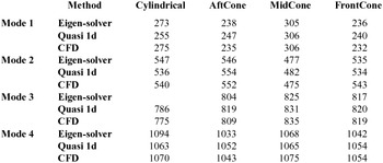
Table 1 Operating conditions for the tests

In addition to the test geometries, more realistic motor geometries of roughly the same length and with initial four-fin finocyl and reverse finocyl grain configurations are also considered for testing the quasi-1D tools. The grain geometries after few seconds of burning are considered here. One eighth of the flow geometry of the former is shown in Fig. 5, and its axial variations of the cross-sectional area and the perimeter of the grain surface are shown in Fig. 6. A structured mesh is used for discretising the domain. The mesh near the nozzle entrance is shown in Fig. 7. The axial variations of cross-sectional areas and burning perimeters for the two cases are shown in Fig. 6. The 3D simulations are also conducted with the same parameter values, except for the burn rates, which are adjusted to achieve target mean chamber pressures.

Figure 5. Geometry of the a solid rocket motor (one-eighth sector) with initial finocyl grain geometry after few seconds of burning (a) whole length and (b) zoomed-in view of fin region.

Figure 6. Axial variations of cross-sectional area and grain perimeter for motors with (a) finocyl and (b) reverse finocyl grain geometries.

Figure 7. Mesh used in 3D simulations close to the nozzle.
4.0 MODE IDENTIFICATION AND DAMPING CALCULATION PROCEDURE
Determination of characteristic mode shapes and damping rates would be difficult when multiple modes are activated. Doing so is considerably easier if only a single mode is activated. Characteristic frequencies, on the other hand, are relatively easier to determine. Starting with a converged steady-state solution, system response to random forcing at the head end in the form fluctuating velocity is simulated. The frequency spectrum of predicted pressure-time data has peaks at characteristic frequencies.
The pressures at several locations have to be noted with time in order to compute frequency spectra. This is because use of the spectra at a single point is problematic. If a single point is chosen and it happens to be a pressure node for one of the modes, the pressure spectra will not show a peak at the frequency corresponding to that particular mode. The head end seems like an ideal choice, but because random forcing is introduced at this end, the spectra tends to be very noisy. The nozzle end of the chamber is also not a perfectly reflecting boundary. This is why spectra at multiple locations are computed so that no peaks are missed.
Smith et al(Reference Smith, Ellis, Xia, Sankaran, Anderson and Merkle31) used a method similar to one used here to identify the eigen-frequencies in a liquid fueled engine. In their work, however, identification of peaks clearly was not possible, so instead of random forcing, they switched to forcing with a combination of multiple frequencies. The forcing frequencies varied from the lowest to the highest in steps of 50 Hz. In the present work, however, locating the peaks seems possible even with random forcing. The difference is perhaps due to the aspect ratio differences between the solid rocket motors and the liquid fuel engines. The lower modes in longer solid rocket motors tend to be primarily axial, and there is no mode coupling with transverse modes. For nearly cylindrical geometries, the characteristic frequencies are integral multiples of the fundamental frequency and can be easily isolated. Even when the geometries are far from cylindrical, the lower characteristic frequencies are well separated.
Even though peaks in the spectra are well separated, the characteristic frequencies are not accurate due to the noise associated with use of white noise forcing and a rather small time step. Using the rough estimate of a frequency peak obtained through random forcing, the velocity at the head end is varied sinusoidally with a small amplitude. Only the mode corresponding to that particular frequency is activated. The fluctuating component of the pressure upon saturation provides the mode shape.
After saturation, the forcing is switched off and decay of a single mode is simulated. By fitting the head-end pressure signal with a decaying sine wave, estimates of frequency and damping rate are obtained. This frequency may be slightly different from one used for forcing because the response to random forcing provides only a rough estimate. The frequency obtained during damping can be used to simulate monochromatic forcing followed by decay again. This kind of iterative procedure eventually leads to an accurate estimate of the characteristic frequency. This iterative procedure is, however, not usually necessary because, in all cases discussed here, the frequency estimated from the first decay simulation is within
 $0.5\,\text{Hz}$
of the final converged value.
$0.5\,\text{Hz}$
of the final converged value.
The procedure outlined above is followed in case of multi-dimensional simulations as well. The results may, however, turn out to be different. Forcing is purely axial in the former. In multi-dimensional simulations, the forcing at the head-end plane is multi-dimensional. Therefore, the lateral modes may also get excited. As seen later, the amplitude of such modes are very small for the geometries chosen here, and no distinct peaks corresponding to them show up in frequency spectra. The identifiable peak locations are close to those in the frequency spectra of quasi-1D results.
The CFD spectra will also capture peaks corresponding to vortex shedding, if any exist. This study actually started with geometries with much steeper cone angles. The CFD spectra showed additional peaks that were missing from those resulting from quasi-1D simulations. The frequencies were too low to be associated with transverse acoustic modes. Vortex shedding was clearly evident upon close examination of the vorticity fields. Vortex shedding is one of the considerations while designing grain geometries for rocket motors. Abrupt or steep changes in area are generally avoided to prevent vortex shedding. The area variations in the geometries finalised for this study are more representative of practical designs.
In linear theory, each mode decays monochromatically. The amplitude decays exponentially. Pressure perturbation corresponding to a single mode decays as follows.
 $$\begin{equation}
p^{\prime }(t;x)=p_o \psi (x) e^{\alpha t}\sin (\omega t)
\end{equation}$$
$$\begin{equation}
p^{\prime }(t;x)=p_o \psi (x) e^{\alpha t}\sin (\omega t)
\end{equation}$$
ψ(x) is the mode shape and po is the initial amplitude. The value of α is negative for a damping signal. The net damping rate has contributions due to flow turning, nozzle radiation and convection through the nozzle.
 $$\begin{equation}
\alpha =\alpha _{FT}+\alpha _{NR}+\alpha _{NC}
\end{equation}$$
$$\begin{equation}
\alpha =\alpha _{FT}+\alpha _{NR}+\alpha _{NC}
\end{equation}$$
By fitting a decaying sine-wave to the pressure signal predicted in simulations after turning off the monochromatic forcing at head end after saturation, the net decay rate can be obtained. Vuillot and Cassalis(Reference Vuillot and Casalis22) provide theoretically derived expressions for each of the individual contributions. The mode shapes required in these expressions can be obtained using the eigen-solver. The latter approach based on a combination of a steady-state ballistics code, eigen-solver and these expressions provides an alternative to simulation-based approaches. The simulation-based approaches are simple but expensive due the fact that isolation and estimation of decay rate have to be done separately for each mode.
The flow-turning loss is calculated using the following expression.
 $$\begin{equation}
\alpha _{FT}=\frac{a}{2 k_N^2 E_N^2} \int \limits _{S_{\mbox{inj}}} \bar{M_{\mbox{{inj}}}} \left(\frac{d \hat{p}_N}{dx}\right)^{2}dS,
\end{equation}$$
$$\begin{equation}
\alpha _{FT}=\frac{a}{2 k_N^2 E_N^2} \int \limits _{S_{\mbox{inj}}} \bar{M_{\mbox{{inj}}}} \left(\frac{d \hat{p}_N}{dx}\right)^{2}dS,
\end{equation}$$
where
- α FT
-
is the flow-turning loss
- a
-
is the average acoustic velocity
- kN
-
is the wave number in radians per unit length, that is,
 $k_N=q\frac{\pi }{L}$
- q
-
is the mode number 1, 2, . . .
-
$\hat{p_N}$
-
is the mode shape of the pressure fluctuation
- EN
-
is the pressure energy defined as
$E_N^2=\int \limits _\Omega \hat{p_N}^2dV$
- Ω
-
is the motor cavity
- M inj
-
is the injection Mach number


Calculation of αFT requires numerical evaluation of a volume integral and a surface integral over the burning surface. The axisymmetric domains in this current study are discretised into disks and integration is performed using trapezoidal rule.
The convection and the radiation losses due to a choked nozzle are calculated using the following expressions, respectively.
 $$\begin{equation}
\alpha _{NC}= a \bar{M_L} \frac{\int \limits _{S_L}\hat{p_N}^2 dS}{2 E_N^2} ,
\end{equation}$$
$$\begin{equation}
\alpha _{NC}= a \bar{M_L} \frac{\int \limits _{S_L}\hat{p_N}^2 dS}{2 E_N^2} ,
\end{equation}$$
 $$\begin{equation}
\alpha _{NR}= a \mathcal {R}(A_L) \frac{\int \limits _{S_L}\hat{p_N}^2 dS}{2 E_N^2},
\end{equation}$$
$$\begin{equation}
\alpha _{NR}= a \mathcal {R}(A_L) \frac{\int \limits _{S_L}\hat{p_N}^2 dS}{2 E_N^2},
\end{equation}$$
where, in addition to the terms mentioned above,
- ML
-
is the Mach number at the entry to the nozzle
- SL
-
is the area of the nozzle entry plane
-
$\mathcal {R}(A_L)$
-
is the nozzle admittance, which for a short nozzle is
$\mathcal {R}(A_L)=\frac{\gamma -1}{2}M_L$

The nozzle loss involves integration on the nozzle entry plane, in addition to the volume integral for the acoustic energy. In both the above nozzle damping terms, the value of the modal function value is obtained from the eigen-solver, which is assumed to be constant at the nozzle entry plane. Hence, the above equations reduce to much simpler forms.
 $$\begin{equation}
\alpha _{NC}= a \bar{M_L} \frac{S_L \hat{p_N}^2 }{2 E_N^2},
\end{equation}$$
$$\begin{equation}
\alpha _{NC}= a \bar{M_L} \frac{S_L \hat{p_N}^2 }{2 E_N^2},
\end{equation}$$
 $$\begin{equation}
\alpha _{NR}= a \mathcal {R}(A_L) \frac{S_L \hat{p_N}^2}{2 E_N^2}
\end{equation}$$
$$\begin{equation}
\alpha _{NR}= a \mathcal {R}(A_L) \frac{S_L \hat{p_N}^2}{2 E_N^2}
\end{equation}$$
5.0 RESULTS AND DISCUSSIONS
Modal frequencies and shapes of the lower modes computed using different approaches are compared first before presenting damping calculations. This comparison would be useful for testing the quasi-1D approximation made in two of the approaches adopted here. Obviously, transverse modes are expected to have higher frequencies and lower modes are all primarily axial, but there is a possibility of coupled axial-transverse modes that needs to be checked.
5.1 Characteristic frequencies and mode shapes
The frequency responses predicted using the two simulation based approaches for the Midcone geometry are shown in Fig. 8. This geometry has been chosen to highlight the fact that frequencies of higher modes need not be integral multiples of the fundamental frequency. In this case more than others, approximating characteristic frequencies using constant area pipe harmonics would be highly erroneous.

Figure 8. Frequency response of motor with Midcone geometry to random noise as predicted by (a) multidimensional CFD (b) quasi-1D model.
Table 2 compares the lowest four characteristic frequencies resulting from various approaches. The frequency spectra based on quasi-1D predictions, in general, tends to be noisy due to use of a very small time step, which makes it difficult to pick out the peaks. Only rough estimates of the characteristic frequencies can be obtained from this approach. More accurate estimates can be obtained by filtering out high frequencies before calculating the spectra or by using simulations of using monochromatic forcing and iterative adjustment. These exercises are, as explained previously, not necessary because frequencies estimated from damping simulations turn out to be very accurate.
Table 2 Summary of modal frequencies
The first and second mode shapes resulting from the three approaches are compared in Figs 9 and 10, respectively. The peak magnitudes are normalised to unity for convenience.

Figure 9. Mode shapes for the first mode for different geometries.

Figure 10. Mode shapes for the second mode for different geometries.
The first mode shapes predicted by the three approaches for any given geometry coincide almost exactly, while the predictions for the second mode differ slightly at the nozzle end. One surprise in these results is that the predictions of the eigen-solver and CFD match very well and differ from quasi-1D code results. The effects of the nozzle are present in both simulation-based approaches, so the results of these two approaches should have actually been closer to each other. This issue will be analysed further in the future.
One crucial point to be noted is that the mode shapes are not always symmetric. In general, zones of larger area have smaller amplitudes. This feature plays a critical role in determining the overall damping rate. Use of symmetric mode shape (assuming cosine function shaped modes) would lead to significant errors.
5.2 Damping rates
The head-end pressure profiles predicted by the two (multi-dimensional CFD and quasi-1D) solvers during the first mode decay in the AftCone geometry are shown in Fig. 11. Also shown are the decaying sine wave fits to the predictions. The corresponding plots for the second mode decay are shown in Fig. 12. Multi-mode decay was predicted in simulations of Afroz and Chakraborty(Reference Javed and Chakraborty20) due to use of cosine function for the mode shape in a non-cylindrical geometry. With the procedure outlined here to isolate a single mode, decay at a single frequency is predicted.
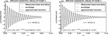
Figure 11. Decay of first mode in the AftCone geometry as predicted by (a) multi-dimensional solver and (b) quas-1D model.

Figure 12. Decay of second mode in the AftCone geometry as predicted by (a) multi-dimensional solver and (b) quas-1D model.
The decay rates computed using the three approaches are summarised in Table 3.
Table 3 Summary of damping rates
For the first mode, both simulations predict similar decay rates in all cases. The maximum difference is less than 1%. For the second mode, however, the maximum difference grows to about 5%. The analytical approach though quite different in terms of predictions provides reasonable first-cut estimates of the damping rates.
It must be noted here that the cylindrical case should not be compared at face value with the others, since the injection velocity in this case is larger to compensate for the lower burning area, to be able to maintain roughly the same mean chamber pressure across the cases.
The predictions of the analytical approach of Vuillot and Casalis(Reference Vuillot and Casalis22) differ by as much as 15%–20% from corresponding flow solver-based predictions. One known source of the error is the use of pseuso-steady-state (short nozzle) assumption for nozzle admittance in calculation of radiative loss term. Measured values of nozzle admittance have been reported to be higher(Reference Zinn32) than estimates based on this assumption.
A glaring observation is that the Aftcone geometry has much lower damping for both the modes. The Midcone geometry has greater damping for the first mode but a lower value for the second mode as compared to the Frontcone. The Aftcone geometry has less than half the damping of both the others. This effect needs to be understood. Based on the fact that analytical approach roughly predicts the trends correctly (i.e. the damping of the Aftcone is far lower than the other two), it can be used to explain the observations.
The modal frequencies of the two approaches obtained from the fitting procedure are tabulated and compared in Table 4. There is an extremely good match between the two methods. The differences are much smaller here compared to those resulting from random forcing and peak identification. This shows that the quasi-1D model is as reliable as the complete CFD in predicting the acoustic frequencies.
Table 4 Summary of modal frequencies during damping
Various contributions to damping are listed separately in Fig. 13. The highest contribution to the damping comes from the convection at the nozzle end, followed by the flow-turning loss, and finally the nozzle radiative losses. It is the nozzle damping component which becomes small in the case of the Aftcone geometry as compared to the other two, in fact, this component is almost one fourth of the other two.
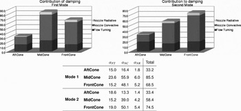
Figure 13. Contribution to the losses from different mechanisms.
To understand the effect of the pressure fluctuations at the nozzle end, the theoretical expression for nozzle damping is reproduced here.
 $$\begin{equation}
\alpha _{NC}= a \bar{M_L} \frac{S_L \hat{p_N}^2 }{2 E_N^2}
\end{equation}$$
$$\begin{equation}
\alpha _{NC}= a \bar{M_L} \frac{S_L \hat{p_N}^2 }{2 E_N^2}
\end{equation}$$
The mass flux for all the cases is roughly the same because the propellant burn rate and the surface area of the burning is equal in all cases. This implies that on the exit plane
 $\dot{m} = \rho _L S_L U_L$
is roughly the same for all the three geometries. Out of this, the density is also not different for the three geometries, because the chamber pressure is the same, as is the temperature. Hence, it is expected that SLUL
is roughly same for all the three geometries. This implies that aMLSL
in Equation (21) must be roughly the same for all the three geometries. Even if ML
of the AftCone is smaller than in the others, the greater area at the nozzle end compensates for this.
$\dot{m} = \rho _L S_L U_L$
is roughly the same for all the three geometries. Out of this, the density is also not different for the three geometries, because the chamber pressure is the same, as is the temperature. Hence, it is expected that SLUL
is roughly same for all the three geometries. This implies that aMLSL
in Equation (21) must be roughly the same for all the three geometries. Even if ML
of the AftCone is smaller than in the others, the greater area at the nozzle end compensates for this.
The main difference, however, comes in the value of
 $\hat{p_N}$
at the nozzle entrance. For the first mode, the value of the
$\hat{p_N}$
at the nozzle entrance. For the first mode, the value of the
 $\hat{p_N}$
for the Aftcone geometry is about 57% of the corresponding values of other geometries. Since this appears as the square in the expression, the numerator in the above equations is much smaller for this geometry. Physically, this may be understood in the following way: the larger the area, the smaller the magnitude of the fluctuation of pressure. This is clearly seen from the mode shape diagrams as well as from the conservation of momentum point of view. The Aftcone geometry with highest area at the nozzle entry plane has the smallest fluctuations at the nozzle end. The smaller the fluctuations, the smaller are the fluctuating energy convected out of the nozzle and the damping. To increase the damping, it is the best to have the largest fluctuations at the nozzle entry plane so that the maximum energy may be convected out. Blomshield(Reference Blomshield, Mathes, Crump, Beiter and Beckstead2,Reference Blomshield, Crump, Mathes, Stalnaker and Beckstead33) has noted this point while explaining why star-forward geometry is more stable than the star-aft geometry in his analysis, although he later(Reference Blomshield1) added velocity coupling and distributed combustion also as contributing factors.
$\hat{p_N}$
for the Aftcone geometry is about 57% of the corresponding values of other geometries. Since this appears as the square in the expression, the numerator in the above equations is much smaller for this geometry. Physically, this may be understood in the following way: the larger the area, the smaller the magnitude of the fluctuation of pressure. This is clearly seen from the mode shape diagrams as well as from the conservation of momentum point of view. The Aftcone geometry with highest area at the nozzle entry plane has the smallest fluctuations at the nozzle end. The smaller the fluctuations, the smaller are the fluctuating energy convected out of the nozzle and the damping. To increase the damping, it is the best to have the largest fluctuations at the nozzle entry plane so that the maximum energy may be convected out. Blomshield(Reference Blomshield, Mathes, Crump, Beiter and Beckstead2,Reference Blomshield, Crump, Mathes, Stalnaker and Beckstead33) has noted this point while explaining why star-forward geometry is more stable than the star-aft geometry in his analysis, although he later(Reference Blomshield1) added velocity coupling and distributed combustion also as contributing factors.
Koreki et al(Reference Koreki, Aoki, Shirota, Toda and Kuratani5) also prescribed grain shapes converging towards the nozzle end for increased stability. They also observed that steeper area transitions are beneficial in such configurations but detrimental in case of diverging grain configurations. Similar observations were made in a computational study by Baczynski et al(Reference Baczynski and Greatrix13). The prescription of lower area at the nozzle end also seems to be applicable in avoiding pulse triggering instabilities(Reference Golafshani, Farshchi and Ghassemi6). Although such instabilities are non-linear, the nozzle damping mechanism remains the same. These observations being consistent with those of this study prove the usefulness of the quasi-1D tools.
The flow-turning loss has been known to depend on where the mass is added into the bulk flow(Reference Matta and Zinn17). It is evident from Equation (16) that flow-turning loss is maximum when combustion adds more mass where the pressure gradient is maximum (i.e. pressure node). The Midcone geometry has more burning area in the middle; therefore, the damping rate of the fundamental mode due to flow turning is the highest among all geometries. The second mode shape in this geometry is almost symmetric, and the pressure gradient is near zero at the center, so its flow-turning loss contribution is much lower.
Another, albeit smaller, effect comes from the value of the denominator (i.e. EN ). EN is evaluated from the expression
 $$\begin{equation}
E_N^2=\int \limits _\Omega \hat{p}_N^2dV
\end{equation}$$
$$\begin{equation}
E_N^2=\int \limits _\Omega \hat{p}_N^2dV
\end{equation}$$
A smaller value of this integral will increase the damping. Observe the shape difference in the mode shapes of the different geometries shown in Fig. 14.

Figure 14. Comparison of first modes in various geometries.
It is evident that in the region where the pressure mode has a large value, having a larger area increases the integral and hence reduces the damping. Hence, it is preferable to have a greater volume of port where the pressure mode has the smallest value. Figure 14 shows that only the Midcone case satisfies this criteria for the first mode. This integral is about 10% lower in the case of Midcone when compared to other geometries. Note that Blomshield(Reference Blomshield1) also prescribed more burning area in the middle, but that was based on combustion, a driving mechanism. Having more area where pressure oscillations are minimal (at least in case of first mode) lower the overall driving force. The damping effect of such a configuration is an independent, additional benefit.
5.3 Realistic small rocket motor geometry
The frequency response to white noise in the motor geometry is plotted in Fig. 15. In this case, the first two peaks correspond to 226 Hz and 524 Hz. Using this lower frequency for forcing, the first mode is activated and its decay is simulated using both 3D CFD and quasi-1D solvers. The predicted head-end pressures are shown in Fig. 16. The frequency and decay rate resulting from fitting these curves with decaying sine waves are also noted in both cases. The predictions of these quantities differ by less than 2% and 3%, respectively.

Figure 15. Frequency spectrum of the motor with finocyl grain due to white noise forcing.

Figure 16. Pressure profiles predicted for the motor with finocyl grain geometry along with corresponding decaying sine-wave fits. The frequency and decay rate of the fit are noted in the legends.
For the case of reverse finocyl grain, the quasi-1D code’s frequency prediction of 218.6 Hz is very close to 217.1 Hz, a value predicted by the 3D simulations. The decay rates predictions of 63.6/s and 64.0/s are also very close to each other.
6.0 CONCLUSIONS
The present work provides with very useful insights into the mechanisms of damping in solid propellant rocket motors from different perspectives. The following is a summary of the observations:
-
1. The frequency of oscillations changes quite dramatically with the geometry. Given same length of the motor, for the cylindrical grain the frequency is roughly 266 Hz, quite close to the pipe harmonics frequency, the frequency of the Aftcone and the Frontcone geometries is about 238 Hz (about 10% lower) and that of the Midcone is about 305 Hz (about 14% greater). This range of about 25% is dependent on the area ratio of the larger to the smaller portions. Thus, it is clear that the geometry of the grain can be designed to have different characteristic frequencies.
-
2. The modes for a non-cylindrical grain are far from the pipe harmonics. Assuming a cosine mode shape for a generic grain is bound to induce errors. The differences in the observed damping rates between the grain geometries can be attributed to the mode shape.
-
3. The modal function value at the nozzle entry is a very important parameter in determining nozzle damping. Higher the relative pressure mode value at the nozzle entry plane, greater the damping. This fact is perhaps the single most important parameter to be incorporated in the design of rocket motors, because the largest source of damping in the class of motors studied is often the nozzle damping.
-
4. The analytical expressions of Vuillot and Casalis(Reference Vuillot and Casalis22), when performed using the correct mode shape, provide very quick rough estimates of the damping rates.
-
5. The observations on grain geometry effects in present work are in line with past experimental(Reference Koreki, Aoki, Shirota, Toda and Kuratani5,Reference Golafshani, Farshchi and Ghassemi6) and numerical(Reference Baczynski and Greatrix11,Reference Baczynski and Greatrix13) studies. The effect of steepness of area variations has not been explored in the present work but is planned for the future. The recommendations regarding the grain geometry made here are based only on damping considerations and combustion effects have not been considered. Some of the recommendations of Blomshield(Reference Blomshield1) are based on combustion. It is interesting that these two set of recommendations are mostly in line with each other.
-
6. The quasi-1D code predicts damping as that of CFD in most cases and almost the exact frequencies as that of CFD. The quasi-1D code takes a small fraction of the time as that of a complete CFD code, which makes the former a very good substitute.


