A) Aqueous solutions

In order to perform measurements on samples similar to a biological cell suspension, household salt (mainly sodium chloride) and sugar (mainly sucrose) are dissolved in deionized water in different concentrations. The concentrations are given in % w/w. The samples are then filled into the funnels and the resulting resonances are recorded.

Figure 3 shows the resonant frequency versus quality factor for the three sensors. The changes of resonance caused by the salt solutions (green stars) are similar for all sensors. Increasing the concentration mainly affects the quality factor and to a lower degree also the resonant frequency.

Fig. 3. Measured resonator parameters for different aqueous solutions.

It is worth noting that an increasing salt concentration, i.e. conductivity, has a greater impact on sensors with lower resonant frequency. This is expected since the effect of conductivity on permittivity decreases with frequency. The effect of dissolved sugar (red plus signs) also differs for the sensors, especially regarding the quality factor. The resonant frequency increases for all sensors, while the quality factor decreases for Sensor 1 but increases for Sensor 3. The quality factor of Sensor 2 is hardly affected. This indicates, at least for higher frequencies, that the dissolved sugar, a non-ionic but slightly polar molecule, reduces permittivity and even loss of the solution. These results are in agreement with measurements on sucrose solutions performed by Kent in similar frequency ranges [Reference Kent and Kress-Rogers17].

In order to estimate reproducibility, each solution is measured several times. A new sample is used in each measurement, i.e. the funnel is emptied and refilled between all measurements. The plots show the average values for each solution.

The error sources in this setup can be separated into three different groups.

The first error source is the electrical noise inherent to the network analyzer. Secondly, the solutions themselves may not be perfectly homogeneous, so that the samples can be slightly different from each other. This can be seen as a chemical error. Thirdly, the funnel structure is not perfectly sealed and the surface is not perfectly smooth. The elastic rubber seal may allow for some of the liquid to creep into the small gaps at the junctions of different materials and surface roughness can hinder wetting of the surface around the sensing tip. The resulting errors are thus due to mechanical inaccuracies.

The three error sources can be evaluated by the recorded resonator parameters for the sample air, water, and saline solutions. The encountered standard deviations for Sensor 1 are given in Table 3. For air samples, the only error that can occur the electrical noise since the other two error sources do not apply here. The deviation of resonant frequency is lower than numerical accuracy used in the evaluation. The standard deviation of the quality factor is also very low (0.1%). For the water samples, the mechanical inaccuracies also play a role, but not the chemical ones, since deionized water is homogeneous. As can be seen in Table 3, the deviations are significantly larger for water samples compared to air. It is obvious that the electrical noise is small compared to the mechanical inaccuracies. The saline solutions also include chemical inaccuracies. However, the encountered deviations are lower than water samples. This indicates that the chemical inaccuracies are also negligible, which is expected at concentrations much lower than in a saturated solution.

Table 3. Standard deviations of resonant frequencies and quality factors encountered in measurements with air, water, and saline solution samples with Sensor 1 for error discussion.

The measured resonances show that the sensors can discriminate between different concentrations. The salt concentration is most easily determined at lower frequencies because of the higher influence of ions on permittivity. The sugar solutions can be discriminated best at higher frequencies because of strong influence on resonant frequency.

All in all, the quality factors are drastically lower when measuring aqueous solutions than with an air sample (compare Table 2). This is caused by high losses of water at microwave frequencies and by strong coupling between the sensor and the sample which is necessary for high sensitivity. The loss tangent of water according to the well established Debye model increases by up to almost 2 in the higher GHz range [Reference Kaatze18]. Therefore, resonant sensors such as these may be less suitable for measurements on biological substances at even higher frequencies since the quality factor of the sensors will be extremely low leading to difficulties in evaluation of the resonance.

B) Evaluation based on perturbation theory

In order to obtain quantitative results for measured permittivity, a perturbation approach is chosen. The change of resonance of microwave near-field sensors can be described by perturbation theory because field changes occur only in the small sampling volume at the tip. The frequency shift of a dielectric (non-magnetic) perturbation, in this case the sample with a relative permittivity ε_r, is given by [Reference Pozar19]

(1)$${{f_1 - f_0} \over {f_0}} \approx - {{\displaystyle{{\vint\int\vint_{V_{s}} \epsilon_0 \lpar \epsilon_{{r}1} - \epsilon_{{r}0} \rpar {\bi E}_1 {\bi E}_0^ {\ast} dV }}} \over \displaystyle{\vint\int\vint_{V_{res}} \epsilon \vert {\bi E}_0 \vert ^2+\mu \vert {\bi H}_0 \vert ^2 dV} \; },$$

where V _s is the sampling volume of the sensor and V _res is the total resonator volume. The subscripts 0 and 1 of frequency f, relative permittivity ε_r, and electric field vector E refer to the unperturbed and the perturbed scenario, respectively. The material inside the resonator has permittivity ε = ε₀ε_r,res and permeability μ = μ₀μ_r,res.

Since the permittivity of aqueous solutions and cell suspensions is close to that of water, some approximations can be made. First, for a homogeneous sample relative permittivity can be pulled out from the integral. Second, since the permittivity changes only slightly, the perturbed electrical field E₁ can be assumed to be equal for all aqueous samples. The unperturbed sensor refers to an empty funnel, i.e. ε_r0 = 1 (air). The reference permittivity of water ε_r1 = ε_r,water (f _r) for the integral can be calculated from the Debye model

(2)$$\displaystyle{\epsilon_{r\comma water}\lpar f\rpar =\epsilon_{\infty\comma water}+\displaystyle{{\epsilon_{0\comma water} - \epsilon _{\infty\comma water}} \over {\displaystyle{1 - j2{\rm \pi}\tau _{water}f}}}}$$

for each sensor at the respective resonant frequency. The static and high-frequency permittivities ε_0,water and ε_∞,water as well as the relaxation time τ_water in equation (2) are determined using the equations developed in [Reference Stogryn15] at 20°C. The volume integral over the electric and magnetic energy in the sensor

(3)$$\displaystyle{{\vint\int\vint_{V_s } \epsilon _0 {\bi E}_{{water}} {\bi E}_0^ {\ast} dV} \over {\displaystyle{\vint\int\vint_{V_{res}} \epsilon \vert {\bi E}_0 \vert ^2+\mu \vert {\bi H}_0 \vert ^2 dV}}}={\displaystyle{{f_0 - f_{water}} \over {f_0 \lpar \epsilon _{r\comma water} - 1\rpar }}=C}$$

is assumed to be equal for different aqueous samples.

In equation (3), the resonant frequency can be substituted by the equivalent complex resonant frequency [Reference Collin20]

(4)$$f_{cr\comma i}=f_{r\comma i} \left({1+j\displaystyle{1 \over {2Q_{0\comma i}}}} \right).$$

Here, subscript i refers to the sample in the funnel, i.e. air, water, etc.

Using the complex permittivities and resonant frequencies of air and water, C can be calculated from equation (3). The complex resonant frequencies of air and water and the resulting complex Cs are listed in Table 4. The complex permittivity ε_r,s of a sample loaded in the funnel is obtained from

(5)$$\epsilon_{r\comma s}=\epsilon_{r\comma s}^{\prime} - j \epsilon_{r\comma s}^{\prime \prime}=\,\displaystyle{{f_{c\comma 0} - f_{c\comma s}} \over {f_{c\comma 0}C}}+1\comma \;$$

Table 4. Complex resonant frequencies and constants C used in the perturbation approach for calculation of complex permittivity.

with f _c,s the measured complex resonant frequency of the sensor. In the following, the real part of complex permittivity ε_r′ will be referred to as permittivity and the imaginary part ε_r″ as loss factor.

The frequency dependent complex permittivity of deionized water and saline solutions is well known from the literature. The values given in the following refer to the results of Stogryn in [Reference Stogryn15].

The accuracy of the approach is estimated by comparing the calculated and the reference permittivities. The values from the measurement and the literature are shown in Fig. 4. Obviously, the accuracy of the approximation decreases for higher salt concentrations. However, for salt concentrations below 1%, the deviation to the reference value is lower than 3% for all sensors except Sensor 1, for which the error is higher (5.4%) for the loss. The reason for this is the large change of the loss at 3 GHz due to increased conductivity. When increasing the conductivity, the field distribution changes slightly compared to the case with a water sample. Thus, the assumptions made in equation (3) become less accurate, which leads to some error.

Fig. 4. Measured and reference [Reference Stogryn15] permittivity values for different saline solutions.

Previous measurements on cell suspensions have shown that permittivity in the frequency range considered here is quite close to that of water, while the loss is decreased by a factor of up to two [Reference Grenier, Dubuc, Poupot and Fournie21]. This is similar to the contrast encountered in the measurement on saline solutions with Sensor 1, where the loss is increased by more than a factor two. Even though the error is not negligible, an evaluation such as this can thus yield a decent estimation of permittivity of cell suspensions. The permittivity estimations for cell suspensions examined in the following can be expected to be within approximately 5 and 10% of the true value for the real and the imaginary part, respectively.

However, since the slope of the calculated permittivity for saline solutions is quite similar to the reference (see Fig. 4), small dielectric contrasts can still be determined with this method since the errors due to the perturbation approach essentially cancel each other.

A) Different cell concentrations

In a first measurement, living CHO cells in the culture medium are used in the measurement. The following biological protocol was applied to the cells before the experiments. The cell concentration after cultivation is determined using a hemocytometer and trypan blue. The cells are then separated from the used culture medium with a centrifuge and are resuspended in fresh culture medium to obtain the desired concentration. This is performed for each cell concentration. The protocol is schematically described in Fig. 6.

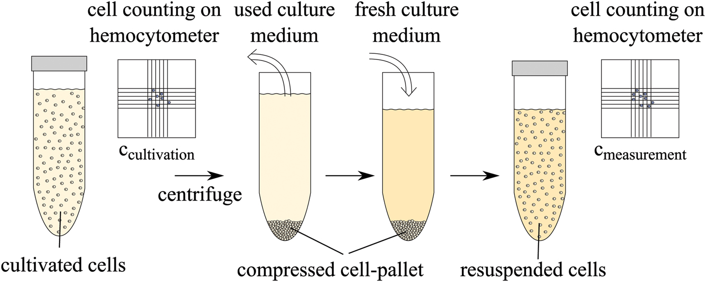
Fig. 6. Biological protocol for preparation of different cell concentrations after cultivation.

Three different concentrations, namely c ₁ = 5 × 10⁶, c ₂ = 10 × 10⁶, and c ₃ = 15 × 10⁶ cells/ml culture medium are inserted into the funnels of the sensors successively. Each sample is measured for 30 minutes in order to allow the cells to sediment at the bottom of the funnel, i.e. on the sensing tip as shown in Fig. 7. The thickness h _s of the sedimented cell layer depends on the cell concentration, i.e. it is higher for larger concentrations. Assuming spherical cells with an average radius of 7 μm and a dense packing of 74% density, the thickness of the sedimented cell layer can be estimated using geometrical considerations. Assuming that 90% of the funnel volume is filled, the volume of the cell suspension is approximately 80 μl. The estimated resulting thickness h _s is given in Table 5 for the three concentrations.

Fig. 7. Sketch of cell behavior in funnel, not to scale. ○1 Plexiglas funnel, sensing tip, seal to prevent leakage, seal to avoid evaporation, cells, evenly distributed, cells, sedimented.

Table 5. Estimated thickness of sedimented cells based on geometrical considerations.

The change of resonance resulting from the sedimenting cells is recorded in intervals of 2 minutes. The results are used to calculate the complex permittivity and are depicted exemplarily in Fig. 8 for Sensors 1 and 2. Both permittivity and loss factor of cell suspension decrease during the experiment. This can be explained by the increased volume percent of cells in the sampling volume which have many components than lower permittivity and loss compared to pure water, such as cell membrane, proteins, organelles, etc. The three concentrations can be distinguished with Sensor 1 but not with the other sensors. The reason for this is the smaller sampling volume of Sensors 2 and 3 which is due to the smaller tip size (see Table 1). The main difference between the three cell suspensions is the layer thickness h _s of the sedimented cells. For Sensor 1, apparently, the sampling volume is higher than h _s since a difference between the suspensions can be observed. For the other sensors, the sampling volume is already filled with the sedimented cells in the suspension with 5 × 10⁶ cells/ml, therefore the increased h _s of the other suspensions does not influence the sensors.

Fig. 8. Complex permittivity of alive cells sedimenting on Sensors 1 and 2 in different concentrations.

The permittivity and loss factor of the sedimented cells, $\bar{\epsilon}_{r\comma sed}^{\prime}$ and $\bar{\epsilon}_{r\comma sed}^{\prime\prime}$, as well as the dielectric change during sedimentation ${\bar \Delta} \epsilon_{r\comma sed}^{\prime}$ and ${\bar \Delta} \epsilon_{r\comma sed}^{\prime\prime}$ are summarized in Table 6 for c = 10 × 10⁶ cells/ml.

Table 6. Permittivity and loss factor of sedimented cells and dielectric change during sedimentation in a cell suspension of c = 10 × 10⁶ cells/ml.

The permittivity of the cell solutions remains below that of water. This is expected because both ionic and non-ionic solvents in the culture medium reduce the permittivity of the liquid as was shown in the experiments with the aqueous solutions (see Fig. 3). The cells also lower the permittivity, as discussed above. The loss factor is lowered by the sedimenting cells, and this effect increases with frequency because the impact of the ions on dissipation decreases.

B) Different vital states

In a second measurement, the dielectric signature of dead cells is investigated. A cell suspension with concentration c ₂ = 10 × 10⁶ cells/ml is prepared using the same protocol as mentioned above. Three samples are taken from the cultivated cells and two of them are ‘killed’ in different ways: one cell suspension is shock-frozen and one is treated with mild heat. The biological protocol is sketched in Fig. 9. Sample 1 contains living cells. Sample 2 is immersed into liquid nitrogen at −196°C. As a result of such a temperature shock, ice crystals form inside the cells and the culture medium and as a result the cell membranes burst [Reference Mazur22]. Thus, after thawing, the cytoplasm of the cells mixes with the culture medium and the remains of the cell membrane and organelles are distributed in the liquid. Sample 3, heated for 10 minutes at 70°C in a thermoshaker, contains dead cells which are still mainly intact, i.e. the cell membrane is not destroyed in this process. The proteins are merely denatured in the heating process which leads to an immediate cell death [Reference Henle and Dethlefsen23].

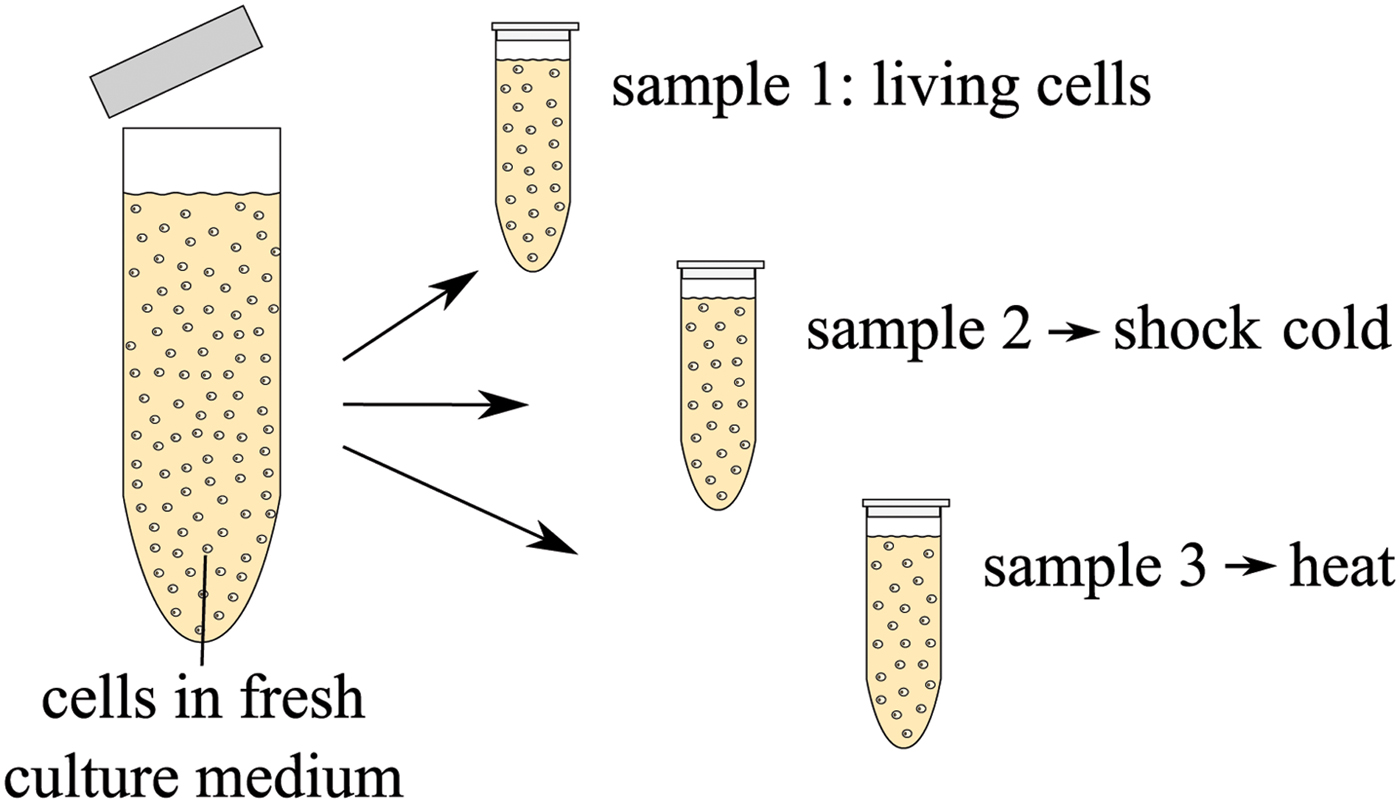
Fig. 9. Biological protocol for preparation of different vital states of cells.

In order to confirm the vital states of the cells, samples of the three cell suspensions are mixed with the vital stain trypan blue. Although the living cells are not colored, dead cells are dyed in dark blue. Photographs taken through a microscope showing the cell suspensions are displayed in Fig. 10. The cells killed with heat are clearly dead but otherwise intact, as expected. In the cell suspension which was shock-frozen, some cells remain alive and some are dead. However, the observed cell concentration is lower in this suspension, since the cells that burst during the frost-thaw cycle are not dyed by the vital stain and are thus not visible.

Fig. 10. Images of different vital states of CHO cell suspensions. The colouring indicates the vital state of the cells: light cells are alive, dark cells are dead. Cell fragments are not coloured, therefore not visible optically.

Prior to the measurements, the cell suspensions are allowed to cool or re-heat to room temperature (20°C), respectively. The different cell suspensions are then filled into the funnels one after the other to sediment on the sensors. The resulting permittivities are shown in Fig. 11 for Sensors 1 and 3. Obviously, the difference between the suspensions affects the loss factor and to a smaller degree also the permittivity. The loss factor of the dead cells is lower than that of the living ones; the values of the frozen cells is between the two other solutions, since both living and dead cells are present in that suspension. This behavior is visible at all three frequencies. The differences Δε_r,dead between the permittivity of sedimented living and dead (heated) cells are listed in Table 7.

Fig. 11. Calculated complex permittivity of cell sedimentation using Sensors 1 and 3. The cell concentration is 10 × 10⁶.

Table 7. Difference between permittivity of living and dead cells observed with the sensors.

The measurements show that the dielectric contrast between living and dead cells is significant. Especially the loss factor can be used to discriminate between different cell suspensions used here. In addition, the experimental results are in agreement with optical observations of the cell suspensions concerning the vitality of the cells in the suspensions. In other measurements in the microwave range with living and dead human umbilical vein endothelial cells, similar observations were made concerning the loss factor of the suspension [Reference Grenier, Dubuc, Poleni, Kumemura, Toshiyoshi, Fujii and Fujita24], i.e. a lowering of the loss factor for dead cells compared to living ones. In that publication, an increase of the permittivity was found for the dead cells, which is not observed here. However, since the cell suspension investigated here is not the same, the diverging observations are most likely found in biological differences between the cell types.