1. Introduction
The Danian–Selandian transition is a period of climatic change. It witnessed two strong depositional changes that can be linked to climatic processes. The first change, dated at 60.3 Ma, is characterized by the onset of continental deposits in Belgium, the formation of channel systems in Tunisia and non-deposition in Egypt (Steurbaut & Sztrákos, Reference Steurbaut and Sztrákos2008). The second change marks the Danian–Selandian boundary (DSB), which was originally defined as the base of the Lellinge Greensand in Denmark and is now defined as the base of the Itzurun Formation in Zumaia, Spain, its Global Boundary Stratotype Section and Point (GSSP), dated at 59.9 Ma (Steurbaut & Sztrákos, Reference Steurbaut and Sztrákos2008; Schmitz et al. Reference Schmitz, Pujalte, Molina, Monechi, Orue-Etxebarria, Speijer, Alegret, Apellaniz, Arenillas, Aubry, Baceta, Berggren, Bernaola, Caballero, Clemmensen, Dinares-Turell, Dupuis, Heilmann-Clausen, Hilario Orus, Knox, Martin-Rubio, Ortiz, Payros, Petrizzo, von Salis, Sprong, Steurbaut and Thomsen2011). The first depositional change corresponds to the P3a/P3b planktonic foraminiferal subzonal boundary and is correlated to a short-term C isotope negative excursion: the Latest Danian Event, or LDE (Bornemann et al. Reference Bornemann, Schulte, Sprong, Steurbaut, Youssef and Speijer2009). This event is one of the first of the Palaeogene hyperthermals, i.e. short-term warming events (Bornemann et al. Reference Bornemann, Schulte, Sprong, Steurbaut, Youssef and Speijer2009; Westerhold et al. Reference Westerhold, Röhl, Donner, McCarren and Zachos2011; Deprez et al. Reference Deprez, Jehle, Bornemann and Speijer2017). The DSB itself is the beginning of climatic fluctuations, with organic and inorganic stable isotope data suggesting a c. 30 kyr hyperthermal event at the very beginning of the Selandian followed by a period of climatic cooling of a few 100 kyr (Storme et al. Reference Storme, Steurbaut, Devleeschouwer, Dupuis, Iacumin, Rochez and Yans2014).
In this paper we aim at understanding the depositional changes and the related climatic events occurring around the DSB from coeval sections using rock-magnetic techniques. Rock-magnetic techniques allow the identification, characterization and quantification of magnetic minerals in rocks by measuring magnetic parameters. These parameters can then be used to understand a wide range of geological processes involving these minerals (e.g. Evans & Heller, Reference Evans and Heller2003). For instance, the goethite over goethite plus haematite ratio (G/(G + H)) can be used to determine humidity levels (Abrajevitch et al. Reference Abrajevitch, der Voo and Rea2009). Anhysteretic remanent magnetization (ARM) can be used to quantify low-coercivity minerals like magnetite, titanomagnetite or greigite (Kodama & Hinnov, Reference Kodama and Hinnov2014), whose origin can be interpreted as detrital or biogenic (Moskowitz et al. Reference Moskowitz, Frankel and Bazylinski1993; Kodama et al. Reference Kodama, Anastasio, Newton, Pares and Hinnov2010). Changes in magnetic mineralogy can thus be interpreted as changes in deposition that can in turn be attributed to climatic changes.
The magnetic susceptibility (MS) is one of the most widely used magnetic proxies. Its fast acquisition allows it to be easily used to study the content of magnetic minerals in sedimentary rocks (e.g. Ellwood et al. Reference Ellwood, Crick and Hassani1999; Mayer & Appel, Reference Mayer and Appel1999; Da Silva et al. Reference Da Silva, De Vleeschouwer, Boulvain, Claeys, Fagel, Humblet, Mabille, Michel, Sardar Abadi, Pas and Dekkers2013; De Vleeschouwer et al. Reference De Vleeschouwer, Boulvain, Da Silva, Pas, Labaye, Claeys, Da Silva, Whalen, Hladil, Chadimova, Chen, Spassov, Boulvain and Devleeschouwer2015). However, the MS of a sample can be influenced by several types of magnetic minerals that show different behaviours (Kodama & Hinnov, Reference Kodama and Hinnov2014); thus, interpreting a MS signal is not always unequivocal. Typically, both paramagnetic and ferromagnetic minerals (ferromagnetic being used sensu lato in this paper) have positive MS values, but for an identical mass the latter have a much higher MS value (Evans & Heller, Reference Evans and Heller2003). Complementary magnetic parameters have to be determined to estimate the contribution to the MS of ferromagnetic, diamagnetic and paramagnetic minerals as well as to provide information about the size, coercivity (i.e. the ability of a ferromagnetic mineral to remain magnetized against an external opposite magnetic field) and type of ferromagnetic minerals. These parameters typically characterize the behaviour of magnetization depending on the magnetic field (e.g. hysteresis loops, isothermal remanent magnetization (IRM)), the temperature or the time.
However, the interpretation of magnetic parameters obtained in weakly magnetic samples such as limestones can be complicated by their high analytical variability. Owing to the low ferromagnetic mineral content in these samples, some of the magnetic parameters will present higher variability than in strongly magnetic materials. Moreover, the magnetic mineralogy may be influenced by a variety of small-scale geological processes that will generate horizontal heterogeneity. This in turn blurs large-scale processes such as the one expected to record climatic variations. This is especially true for parameters influenced by ferromagnetic minerals, as these minerals can form, change and dissolve locally at each step between deposition and cropping out.
The analytical variability of magnetic parameters and the high susceptibility to horizontal heterogeneity make such proxies prone to over-interpretation. Therefore, prior to the depositional changes study, focus will also be set on providing a comprehensive overview of the interpretation of our magnetic parameters, with a focus on the analytical error and on the reproducibility of our results between sections of overlapping age.
Following the work of Storme et al. (Reference Storme, Steurbaut, Devleeschouwer, Dupuis, Iacumin, Rochez and Yans2014), we study here the same three coeval sections spanning the Danian–Selandian transition: Loubieng (France), Zumaia (Spain) and Sidi Nasseur (Tunisia). The goal is to identify, characterize and compare depositional changes in these sections by using magnetic parameters as proxies. The rock-magnetic data obtained for this study are used together with biostratigraphic and δ13Corg data to provide new constraints on the stratigraphic framework and thus on the changes in the sedimentation rates in the Atlantic and the Tethyan sections around the DSB.
2. Geographical and geological setting
2.a. The Zumaia GSSP section
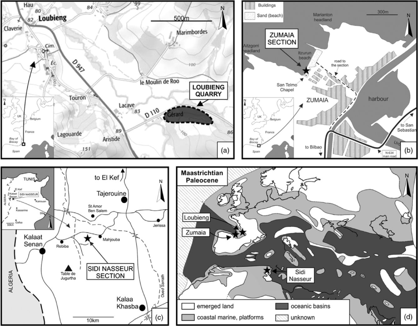
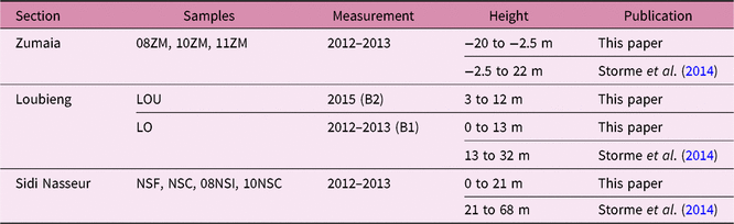
The Zumaia sea-cliff section contains the GSSP for the base of the Selandian Stage (also referred to as the DSB; Schmitz et al. Reference Schmitz, Pujalte, Molina, Monechi, Orue-Etxebarria, Speijer, Alegret, Apellaniz, Arenillas, Aubry, Baceta, Berggren, Bernaola, Caballero, Clemmensen, Dinares-Turell, Dupuis, Heilmann-Clausen, Hilario Orus, Knox, Martin-Rubio, Ortiz, Payros, Petrizzo, von Salis, Sprong, Steurbaut and Thomsen2011). It is located on Itzurun beach, c. 500 m to the northwest of Zumaia city centre, in Spain (43° 18’ 5” N, 2° 15’ 35” W; Fig. 1b; Storme et al. Reference Storme, Steurbaut, Devleeschouwer, Dupuis, Iacumin, Rochez and Yans2014). A long sequence of rocks of Late Cretaceous to early Palaeogene age crop out along the beach, the Palaeocene being represented by 165 m thick hemipelagic deposits (Schmitz et al. Reference Schmitz, Pujalte, Molina, Monechi, Orue-Etxebarria, Speijer, Alegret, Apellaniz, Arenillas, Aubry, Baceta, Berggren, Bernaola, Caballero, Clemmensen, Dinares-Turell, Dupuis, Heilmann-Clausen, Hilario Orus, Knox, Martin-Rubio, Ortiz, Payros, Petrizzo, von Salis, Sprong, Steurbaut and Thomsen2011). The palaeogeographical position of the section is in the Bay of Biscay, in the Atlantic realm (Fig. 1d). The section spans the upper part of the Danian Aitzgorri Limestone Formation and the lower part of the Selandian Itzurun Formation (Schmitz et al. Reference Schmitz, Pujalte, Molina, Monechi, Orue-Etxebarria, Speijer, Alegret, Apellaniz, Arenillas, Aubry, Baceta, Berggren, Bernaola, Caballero, Clemmensen, Dinares-Turell, Dupuis, Heilmann-Clausen, Hilario Orus, Knox, Martin-Rubio, Ortiz, Payros, Petrizzo, von Salis, Sprong, Steurbaut and Thomsen2011). An important lithological change occurs at the boundary between the two formations where the reddish marl of the Selandian overlies the greyish-to-reddish alternating marl and limestone beds of the Danian. This lithological change defines the base of the Selandian (Schmitz et al. Reference Schmitz, Pujalte, Molina, Monechi, Orue-Etxebarria, Speijer, Alegret, Apellaniz, Arenillas, Aubry, Baceta, Berggren, Bernaola, Caballero, Clemmensen, Dinares-Turell, Dupuis, Heilmann-Clausen, Hilario Orus, Knox, Martin-Rubio, Ortiz, Payros, Petrizzo, von Salis, Sprong, Steurbaut and Thomsen2011), and coincides with bio-event E4 (Storme et al. Reference Storme, Steurbaut, Devleeschouwer, Dupuis, Iacumin, Rochez and Yans2014), i.e. the end of the acme of Braarudosphaera and the lowest consistent occurrence of Lithoptychius aff. bitectus (Fasciculithus janii sensu Steurbaut & Sztrákos, Reference Steurbaut and Sztrákos2008). The hemipelagic sediments were deposited at an estimated water depth of between 900 and 1100 m (Arenillas et al. Reference Arenillas, Molina, Ortiz and Schmitz2008). A total of 89 samples were studied here. Some of the C and O stable isotope measurements were already presented in Storme et al. (Reference Storme, Steurbaut, Devleeschouwer, Dupuis, Iacumin, Rochez and Yans2014) (Table 1). The sampling interval is irregular, ranging from 0.10 to 2.75 m.

Fig. 1. Location of the (a) Loubieng (Bureau de Recherches Géologiques et Minières maps database, available at http://infoterre.brgm.fr/viewer/MainTileForward.do; accessed 11 February 2015), (b) Zumaia and (c) Sidi Nasseur sections (Storme et al. Reference Storme, Steurbaut, Devleeschouwer, Dupuis, Iacumin, Rochez and Yans2014). (d) Palaeogeographical context during Maastrichtian and Paleocene times (modified from Gheerbrant & Rage, Reference Gheerbrant and Rage2006 following Storme et al. Reference Storme, Steurbaut, Devleeschouwer, Dupuis, Iacumin, Rochez and Yans2014).
Table 1. Details of C and O isotope analyses
2.b. The Loubieng section
The Loubieng section is located in the North Pyrenean Tectonic Zone westward of Pau, in France (Henry et al. Reference Henry, Zolnaï, Le Pochat and Mondeilh1989; Storme et al. Reference Storme, Steurbaut, Devleeschouwer, Dupuis, Iacumin, Rochez and Yans2014). It is an abandoned quarry located 300 m to the east of the junction between route départementale D947 Orthez–Navarrenx and route départementale D110 Loubieng–Sauvelade (43° 25’ 38” N, 0° 44’ 37” W; Fig. 1a). It is formed by several faulted blocks marked by small displacements along normal faults. It was investigated in the past for biostratigraphy (Peybernès et al. Reference Peybernès, Fondecave-Wallez, Hottinger, Eichène and Segonzac2000; Steurbaut & Sztrákos, Reference Steurbaut and Sztrákos2008; Storme et al. Reference Storme, Steurbaut, Devleeschouwer, Dupuis, Iacumin, Rochez and Yans2014), stable isotopes (Storme et al. Reference Storme, Steurbaut, Devleeschouwer, Dupuis, Iacumin, Rochez and Yans2014) and cyclostratigraphy (Dinarès-Turell et al. Reference Dinarès-Turell, Stoykova, Baceta, Ivanov and Pujalte2010). Palaeomagnetic measurements were carried out; however, the primary remanent magnetization record was overprinted by a consistently reverse component of unknown age blocked in low-coercivity minerals (Dinarès-Turell et al. Reference Dinarès-Turell, Stoykova, Baceta, Ivanov and Pujalte2010). The lower part of the section belongs to the upper part of the Lasseube Formation (Steurbaut & Sztrákos, Reference Steurbaut and Sztrákos2008; Storme et al. Reference Storme, Steurbaut, Devleeschouwer, Dupuis, Iacumin, Rochez and Yans2014). It forms the quarry front and consists of an alternation of almost horizontally bedded limestone beds and marl intercalations. As in Zumaia, the lithology evolves from carbonates to fine-grained siliciclastic deposits from the Danian towards the Selandian. This is most obvious at the boundary between the limestone beds of the Lasseube Formation and the overlying marl and clays of the Pont-Labau Formation (Latapy Member). The DSB has been placed at this formation boundary by Steurbaut & Sztrákos (Reference Steurbaut and Sztrákos2008). It also coincides with bio-event E4 (Storme et al. Reference Storme, Steurbaut, Devleeschouwer, Dupuis, Iacumin, Rochez and Yans2014). The palaeogeographical position of the Loubieng deposits is in the Bay of Biscay, in the Atlantic realm (Fig. 1d; Storme et al. Reference Storme, Steurbaut, Devleeschouwer, Dupuis, Iacumin, Rochez and Yans2014). The depositional depth of the sediments has been estimated to be more than 600 m (Steurbaut & Sztrákos, Reference Steurbaut and Sztrákos2008). A bed-to-bed correlation of the Danian interval between the Loubieng, Zumaia and Bjala (Bulgaria) sections was established by Dinarès-Turell et al. (Reference Dinarès-Turell, Stoykova, Baceta, Ivanov and Pujalte2010) on the basis of lithologic stacking patterns that represent eccentricity orbital cycles, with limestone–marl couplets representing precession cycles.
The first batch of samples (namely, B1) was initially collected in marl and claystone beds by Steurbaut & Sztrákos (Reference Steurbaut and Sztrákos2008). Batch B1 was used for C and O isotope geochemistry and biostratigraphy analyses. Parts of these results were presented in Storme et al. (Reference Storme, Steurbaut, Devleeschouwer, Dupuis, Iacumin, Rochez and Yans2014), and are reworked in this study as part of a larger set of measurements on batch B1 (Table 1). Additionally, we collected samples every 0.10 m through the Danian and basal Selandian, and every 0.25 m in the upper part of the Selandian to provide a second batch of samples (batch B2; Table 1) representative of all lithologies present in the section. Batch B2 contains 266 samples, making Loubieng the most completely sampled section of the three. However, the sampling resolution is not sufficient to allow the robust detection of short-term cycles (Martinez et al. Reference Martinez, Kotov, De Vleeschouwer, Pas and Pälike2016), which is beyond the scope of this study.
2.c. The Sidi Nasseur section
The Sidi Nasseur section is located between Kalaat Senan, Tajerouine and Kalaa Khasba in Tunisia, close to the Algerian border (35° 48’ 18” N, 8° 26’ 48” E; Fig. 1c; Storme et al. Reference Storme, Steurbaut, Devleeschouwer, Dupuis, Iacumin, Rochez and Yans2014). It is a composite section, formed by four subsections (namely, NSC, 10NSC, NSF and 08NSI), exposed on the flank of an incised gully (Storme et al. Reference Storme, Steurbaut, Devleeschouwer, Dupuis, Iacumin, Rochez and Yans2014). The sediments are marl-shales deposited in a neritic environment and form part of the El Haria Formation (Guasti et al. Reference Guasti, Speijer, Brinkhuis, Smit and Steurbaut2006; Van Itterbeeck et al. Reference Van Itterbeeck, Sprong, Dupuis, Speijer and Steurbaut2007). Intercalations of limestone and indurated marl can also be found (Storme et al. Reference Storme, Steurbaut, Devleeschouwer, Dupuis, Iacumin, Rochez and Yans2014). Palaeogeographically it belongs to the southern Tethys realm, near Kasserine island, which supplied significant terrigenous input (Fig. 1d; Guasti et al. Reference Guasti, Speijer, Brinkhuis, Smit and Steurbaut2006). The position of the DSB in the section was proposed at 38.5 m by Storme et al. (Reference Storme, Steurbaut, Devleeschouwer, Dupuis, Iacumin, Rochez and Yans2014) based on the bio-event E4. A total of 149 samples were studied here. Some of them provided C and O stable isotope measurements that were presented in Storme et al. (Reference Storme, Steurbaut, Devleeschouwer, Dupuis, Iacumin, Rochez and Yans2014) (Table 1). The sampling interval is irregular in the lower part of the section (in the NSC, 10NSC and NSF subsections), with a range of from 0.20 to 1.75 m between samples, but the upper part was sampled regularly every 0.25 m (in the 08NSI subsection).
3. Materials and analytical methods
3.a. Biostratigraphy
The foraminiferal and calcareous nannofossil biostratigraphic interpretations of the Zumaia, Sidi Nasseur and Loubieng sections are based on bio-events E1 to E7 as defined by Storme et al. (Reference Storme, Steurbaut, Devleeschouwer, Dupuis, Iacumin, Rochez and Yans2014), essentially relying on Schmitz et al. (Reference Schmitz, Pujalte, Molina, Monechi, Orue-Etxebarria, Speijer, Alegret, Apellaniz, Arenillas, Aubry, Baceta, Berggren, Bernaola, Caballero, Clemmensen, Dinares-Turell, Dupuis, Heilmann-Clausen, Hilario Orus, Knox, Martin-Rubio, Ortiz, Payros, Petrizzo, von Salis, Sprong, Steurbaut and Thomsen2011) for the Zumaia section and on Steurbaut & Sztrákos (Reference Steurbaut and Sztrákos2008) for the Loubieng section. Additional calcareous nannofossil investigations were carried out on six samples from the Loubieng section to pinpoint the second radiation of the fasciculiths (FR2; Schmitz et al. Reference Schmitz, Pujalte, Molina, Monechi, Orue-Etxebarria, Speijer, Alegret, Apellaniz, Arenillas, Aubry, Baceta, Berggren, Bernaola, Caballero, Clemmensen, Dinares-Turell, Dupuis, Heilmann-Clausen, Hilario Orus, Knox, Martin-Rubio, Ortiz, Payros, Petrizzo, von Salis, Sprong, Steurbaut and Thomsen2011), which was not discussed previously for this section, and to verify the position of E5. Four additional samples were collected in the uppermost 2 m of the Danian (25b, 27a, 27c and 27d at 17.73, 18.41, 18.85 and 19.20 m, respectively) and two in the lowermost 9 m of the Selandian (29b at 26.87 m and 32a at 31.5 m). The biozonation and taxonomy adopted here were detailed in Storme et al. (Reference Storme, Steurbaut, Devleeschouwer, Dupuis, Iacumin, Rochez and Yans2014). Smear slides and samples are stored in the collections of the Royal Belgian Institute of Natural Sciences (Brussels, Belgium).
3.b. Sample colour determination
Standard lithological and colour observations were made to use as a reference against the magnetic parameters. Sample colour determination was achieved by visual comparison of humidified samples with a Munsell chart adapted for geological purposes (Goddard et al. Reference Goddard, Trask, De Ford, Rove, Singewald, Overbeck and Overbeck1948). Colours are classified by a code, giving the hue, lightness and chroma, and by a name from the ISCC-NBS classification (in italics in this article). Some sample sections were polished to observe the distribution of colour using optical microscopy.
3.c. Instrumentation for magnetic measurements
Low-field magnetic susceptibility (XLF) was measured with a Kappabridge MFK1-A (AGICO) installed at the Royal Belgian Institute of Natural Sciences (RBINS) and set at a field intensity of 400 A m−1 and a frequency of 976 Hz. The sample mass for these measurements (c. 10 g) was determined with a 1 mg precision weighing scale. Induced and remanent isothermal magnetization curves were measured with an induction coercivity meter (J-meter; Evans & Heller, Reference Evans and Heller2003) at the Royal Meteorological Institute of Belgium (RMIB). The J-meter works in a range of magnetic fields limited to ± 500 mT. Additional magnetic techniques were further performed at much higher magnetic fields to study the influence of high-coercivity minerals on XLF and on the J-meter measurements. The additional analyses were performed using a Magnetic Property Measurement System MPMS 3 (Quantum Design), which is installed at the RMIB and can reach magnetic fields of up to 7 T. In each of the sections, 40 to 55 samples were selected and measured with the J-meter. From those samples measured using the J-meter, 13 were further selected to be studied using the MPMS 3 (four from Zumaia, nine from Loubieng). For these types of measurements, the sample mass was determined using a laboratory weighing scale with a precision of 0.02 mg. Typical sample masses were in the order of 1 g and 25 mg, for the J-meter and the MPMS 3 measurements, respectively. The J-meter measurement sequence is explained in detail in Devleeschouwer et al. (Reference Devleeschouwer, Petitclerc, Spassov and Preat2010).
3.d. Magnetic parameters calculation
3.d.1. Parameters related to magnetic susceptibility
The high-field magnetic susceptibility (XHF) estimates the contribution of diamagnetic and paramagnetic minerals to XLF. XHF is obtained from a linear regression on the induced magnetization curve at high magnetic fields (Equation 1). In this study, the high-field interval ranges from c. 0.3 to c. 0.5 T (the precise interval is adjusted for each sample to avoid artefacts in case of low signal-to-noise (S/N) ratio).
 $${X_{HF}} = {{d{M_i}(H)} \over {{\mu _0}\,dH}}$$
(1)
$${X_{HF}} = {{d{M_i}(H)} \over {{\mu _0}\,dH}}$$
(1)
where Mi is the induced magnetization intensity, H the magnetizing field and µ0 is the magnetic permeability of a vacuum. With the magnetic fields of less than 0.5 T reached by the J-meter, the presence of high-coercivity minerals such as haematite, goethite or pyrrhotite (Dekkers, Reference Dekkers, Gubbins and Herrero-Bervera2007) can also increase the value of XHF. The Xferri parameter quantifies the contribution to XLF of ferrimagnetic (or low-coercivity) minerals such as magnetite, maghaemite and greigite. Xferri is obtained by subtracting XHF (estimating the contribution of diamagnetic, paramagnetic and high-coercivity minerals) from XLF, as the ferrimagnetic minerals are considered saturated in a field above 0.3 T (Dekkers, Reference Dekkers, Gubbins and Herrero-Bervera2007).
3.d.2. Parameters for viscous remanence decay
The viscous remanence decay is the decrease of remanent magnetization with time. It is measured during the final measurement step of the J-meter sequence and is related to the occurrence of magnetically viscous grains, depending on their size. Viscous behaviour can be observed in multidomain (MD) grains, large enough to have several magnetic domains. Magnetic minerals around the superparamagnetic (SP)/stable single domain (SSD) grain-size boundary (c. 20–30 nm at 25 °C) also display viscous behaviour (Néel, Reference Néel1949; Liu et al. Reference Liu, Torrent, Maher, Yu, Deng, Zhu and Zhao2005). In these SP/SSD grains, the viscous effect is usually much more pronounced than in MD grains. Magnetic minerals below the SP/SSD grain-size boundary are superparamagnetic and lose their remanent magnetization before it can reliably be observed with our instruments. Conversely, SSD grains do not show such an effect within typical observation times, i.e. seconds to weeks. This is due to magnetization decay of a magnetic grain following an exponential law in relation to grain size. The overall viscous decay of a sample is quantified by the dimensionless parameter Sd (Dunlop, Reference Dunlop1973; Wang et al. Reference Wang, Løvlie, Zhao, Yang, Jiang and Wang2010):
 $${S_d} = {{d{M_{r\,relative}}(log(t))} \over {dlog(t)}}$$
(2)
$${S_d} = {{d{M_{r\,relative}}(log(t))} \over {dlog(t)}}$$
(2)
where Mr relative is the remanent magnetization intensity normalized to its initial value at 0 s. In the case of the J-meter measurements, the magnetization values were normalized to M(t = 0.4 s), because the magnet needs 0.4 s to drive the field down from 500 to 0 mT. The Sd parameter was calculated here with a similar time interval for all samples, from 0.4 to 100 s.
3.d.3. Parameters related to the saturation of ferromagnetic minerals
The J-meter device can reach fields of up to 0.5 T, which exceed the saturation magnetic field of most of the low-coercivity minerals. This magnetic field is nonetheless not strong enough to saturate the high-coercivity minerals. We define here the ΔIRM and the high-coercivity mineral contribution (HCMC) parameters to estimate their contribution to the IRM at the maximum field available (Devleeschouwer et al. Reference Devleeschouwer, Riquier, Bábek, De Vleeshouwer, Petitclerc, Sterckx, Spassov, Da Silva, Whalen, Hladil, Chadimova, Chen, Spassov, Boulvain and Devleeschouwer2015):
 $${\rm \Delta IRM} = IR{M_{ - 0.5T}} - IR{M_{ - 0.3T}}$$
(3)
$${\rm \Delta IRM} = IR{M_{ - 0.5T}} - IR{M_{ - 0.3T}}$$
(3)
 $$HCMC(\% ) = 100\% *{{\rm \Delta IRM} \over {IR{M_{ - 0.5T}}}}$$
(4)
$$HCMC(\% ) = 100\% *{{\rm \Delta IRM} \over {IR{M_{ - 0.5T}}}}$$
(4)
ΔIRM is not normalized, and should be used compared to the IRM at 0.3 T and/or 0.5 T. Note that high-coercivity minerals can display magnetization over the whole field spectrum and thus contribute to the IRM−0.3 T value (Equation 3). In addition, the maximum available field is limited to 0.5 T; contributions of high-coercivity minerals at higher fields are thus not detected. For these reasons, high values in HCMC and ΔIRM underestimate the actual proportion of high-coercivity minerals and must be considered rather as an approximation of the contribution of high-coercivity minerals to the total remanence of the sample. In this study, HCMC and ΔIRM are calculated from the backfield curve, which justifies the negative magnetic field values used in Equations 3 and 4. This approach allows all samples to go through a similar initial magnetization at 0.5 T and minimizes the effect of any natural remanent magnetization left in the sample at −0.5 T.
3.d.4. Hysteresis parameters
Four parameters usually characterize hysteresis loops: saturation remanent magnetization (Mrs), coercivity of remanence (Hcr), saturation magnetization (Ms) and coercive force (Hc). Mrs and Hcr can be obtained from the remanent magnetization data and are not influenced by dia- and/or paramagnetic contributions. Mrs is equivalent to the IRM−0.5 T if saturation is attained at −0.5 T, and Hcr is obtained by finding the field value at zero remanent magnetization. Usually, Mrs is determined from the hysteresis loop (i.e. from induced magnetization data), but in this study it was calculated from the remanent magnetization at the maximum field of 0.5 T if saturation is reached. This is a more accurate determination because the hysteresis measurement is influenced by the remanent field of the electromagnet. Conversely, remanent magnetization is measured in a magnetically shielded induction coil outside of the electromagnet.
Natural samples often contain significant amounts of dia- and/or paramagnetic minerals, both having a linear induced magnetization dependence to the magnetic field. A high-field slope correction can be applied to induced magnetization data to subtract the contribution of dia- and/or paramagnetic minerals, following Equation 5:
 $${M_{i\,corrected}}(H) = {M_i}(H) - {\mu _0}*H*{X_{HF}}$$
(5)
$${M_{i\,corrected}}(H) = {M_i}(H) - {\mu _0}*H*{X_{HF}}$$
(5)
where Mi corrected is the corrected induced magnetization. From Mi corrected, Ms can then be determined as the Mi corrected at 0.5 T, and Hc as the field value where Mi corrected is zero. This correction only applies when the saturation is reached between 0.3 and 0.5 T. Otherwise, high-coercivity minerals would also contribute to XHF and mislead the correction. If the HCMC exceeds the arbitrarily chosen threshold of 5 %, we consider that saturation is not reached. In that case, the parameters Mrs, Mi corrected, Ms and Hc are incorrect and not taken into account.
3.d.5. Variability and uncertainty calculation
The calculations of the several magnetic parameters used in this study rely on isothermal magnetization curves that are measured with a J-meter. Because of the low magnetic content of the samples, the obtained magnetization curves are relatively noisy, especially for the induced magnetization at high fields. At a field of c. 0.4 T, the S/N ratio is typically about 0.75 for samples with an induced magnetization of 2 to 4 mA m2 kg−1 (typically the limestone samples in this study). The weakest samples have a S/N ratio of c. 0.50. The data is thus smoothed, applying a linear regression on specific magnetic field intervals (e.g. around 0 mT for Mrs, around Hcr, etc.). The magnetic field intervals chosen for smoothing are adapted on a visual basis for each sample to compensate for noise without creating artefacts. The variability of the parameters is different for each sample and is especially high in weakly magnetic samples such as the limestones studied here. To account for this, measurements and parameter calculations were done three times and averaged. The standard deviation of the three samples was calculated using the central limit theorem, allowing the variability of the parameters to be estimated for each sample separately.
3.d.6. High-field (7T) hysteresis
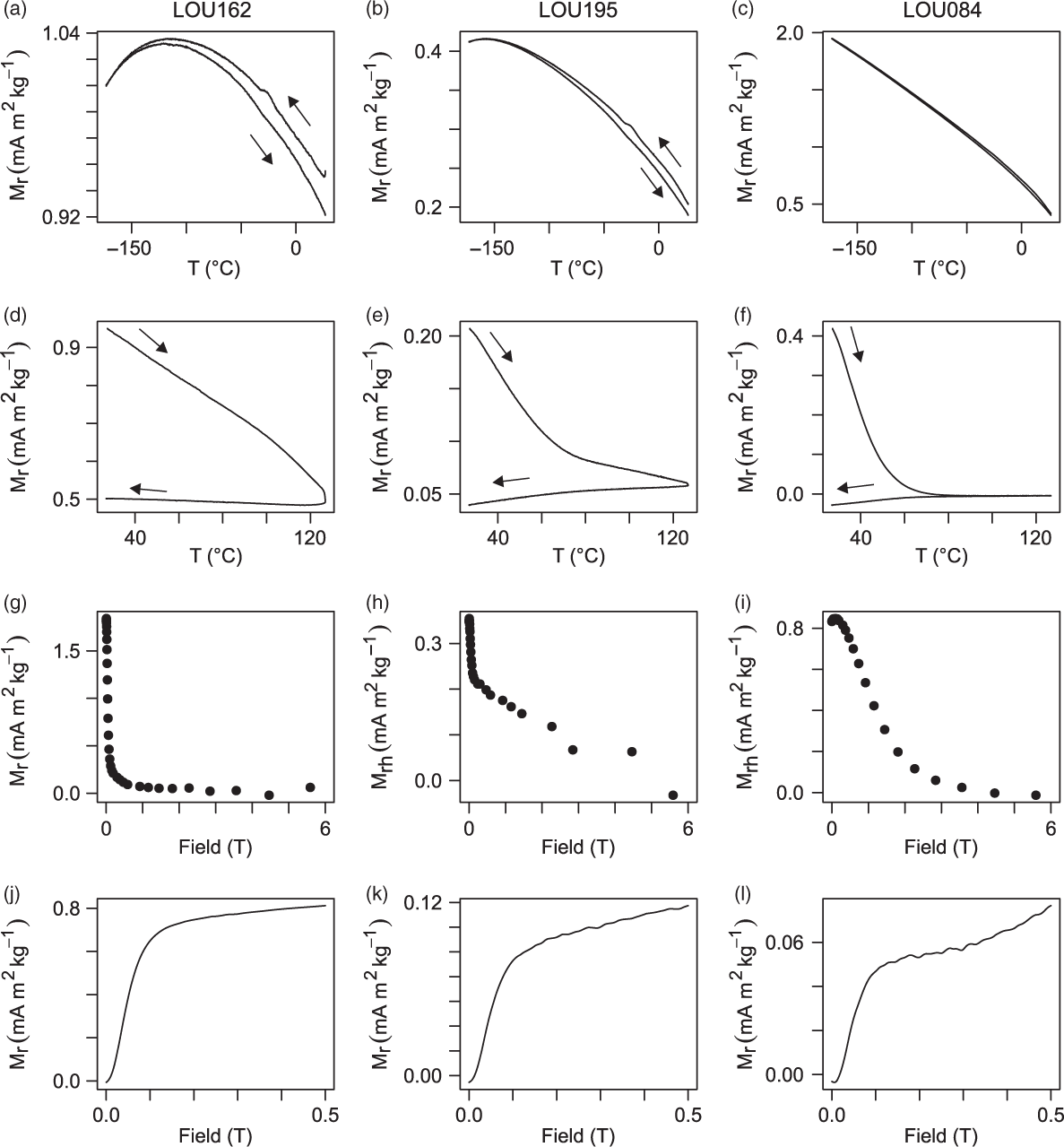
Some samples from the Loubieng and Zumaia sections showed evidence of the presence of high-coercivity minerals. High-field hysteresis loops (up to 7 T) were performed on 13 of these samples to study their saturation at high fields using the remanent hysteretic magnetization (Mrh; Fabian & von Dobeneck, Reference Fabian and von Dobeneck1997):
 $${M_{rh}}(H) = {{{M^ + }(H) - {M^ - }(H)} \over 2}$$
(6)
$${M_{rh}}(H) = {{{M^ + }(H) - {M^ - }(H)} \over 2}$$
(6)
where M+ and M− are the upper and lower branches of the hysteresis. Mrh accounts for the opening of the hysteresis curve and its calculation does not require slope correction (e.g. Fig. 2g–i). If the sample is saturated, the hysteresis loop should be closed and Mrh should stabilize to zero in the high-field ranges.

Fig. 2. Comparison of magnetic analyses of selected samples from Loubieng section, where high-coercivity minerals are present: in sample LOU162 haematite, in sample LOU195 a mixture between haematite and goethite and in sample LOU084 goethite. (a–f) Remanent magnetization versus temperature (measured with the MPMS 3). The small fluctuation observed at −25 °C is interpreted as the Morin transition that is characteristic for haematite. Goethite-bearing samples have a more linear and reversible cooling cycle, and goethite loses its remanence before 80 °C during the warming cycle. (g–i) Mrh of a hysteresis at 7 T (measured with the MPMS 3). Only half of the hysteresis is represented. Goethite samples do not saturate, but in the goethite-dominated sample (LOU084) remanence decreases smoothly well before 6 T. (j–l) IRM of the samples (measured with the J-meter), with a higher coercivity component in LOU084 relative to the other samples (goethite). The partial saturation at 0.3 T also indicates the presence of low-coercivity minerals in all three samples.
3.d.7. Temperature dependence of remanent magnetization
The same 13 samples were analysed for their temperature dependence of remanent magnetization (e.g. Fig. 2a–f). Before measurement, the samples were magnetized at ‘room temperature’ (27 °C or 300 K) in a 7 T field. Then the field was switched off and a waiting time of 10 min was applied to minimize the viscous remanent magnetization contributions to the total remanent magnetization. After that, the remanent magnetization was measured during a low-temperature cycle from 27 °C to −173 °C (300 to 100 K) and back to 27 °C. A second measurement was carried out, during a high-temperature cycle from 27 °C to 127 °C (400 K) and back to 27 °C. The sample was prepared before the second measurement with another 7 T remanence acquisition at 27 °C followed by a 10 min waiting time.
From the latter analysis, the goethite contribution (GC) to the remanent magnetization was calculated. It relies on goethite having an unblocking temperature (Tb) of lower than 110 °C, and on the assumption that the remanence after Tb can be used to approximate the remanence behaviour of haematite and of low-coercivity minerals before Tb (see also Dekkers, Reference Dekkers1989). The unblocking temperature is here used rather than the Néel temperature (120 °C; Özdemir & Dunlop, Reference Özdemir and Dunlop1996), as the latter is too close to the maximum temperature reached by the MPMS 3 (400 K or 127 °C). The remanence between Tb and the maximal temperature that the MPMS 3 reaches (i.e. 127 °C) is modelled by a linear function for which the parameters a and b are determined by linear regression:
 $$M_r^{model}(T) = aT + b$$
(7)
$$M_r^{model}(T) = aT + b$$
(7)
Next, this function was extrapolated to 27 °C and the GC parameter was calculated as follows:
 $$GC = 100\% *{{M_r^{total}(27^\circ C) - M_r^{model}(27^\circ C)} \over {M_r^{total}(27^\circ C)}}$$
(8)
$$GC = 100\% *{{M_r^{total}(27^\circ C) - M_r^{model}(27^\circ C)} \over {M_r^{total}(27^\circ C)}}$$
(8)
3.e. Organic carbon isotope (δ13Corg) measurements
The methodology to measure the δ13Corg is the same as in Storme et al. (Reference Storme, Steurbaut, Devleeschouwer, Dupuis, Iacumin, Rochez and Yans2014): samples were powdered, acidified in 25 % HCl for 2 hours to remove carbonates and centrifuged repeatedly with deionized water until a neutral sediment was obtained. The remainder was dried and powdered again. These treated samples were then weighed in tin capsules, which were rolled into balls and measured for δ13Corg using a Carlo Erba EA1110 elemental analyser coupled to a Thermo Finnigan Delta plus XP mass spectrometer. Carbonates and total organic carbon contents were measured with a Bernard calcimeter and a standard LECO carbon analyser (CS-200), respectively. The variability of repeated δ13Corg measurements was 0.4 ‰ (2σ) on laboratory standards and selected samples.
Two batches of samples were processed and measured separately for organic carbon isotope (δ13Corg) measurements; see Table 1 for further details. As they were measured separately, there might be a slight offset of δ13Corg absolute values between these two batches owing to calibration differences.
4. Results
4.a. Biostratigraphy
4.a.1. Loubieng
The calcareous nannofossil investigation of the six additional samples from the Loubieng section (Fig. 3) confirms the biostratigraphic interpretation of Storme et al. (Reference Storme, Steurbaut, Devleeschouwer, Dupuis, Iacumin, Rochez and Yans2014). The following bio-events are identified (Fig. 3):
Bio-event E2 at 8.95 m. This event coincides with the calcareous nannofossil subzonal NTp7a and NTp7b boundary defined by Varol (Reference Varol, Crux and van Heck1989). It corresponds to the first radiation of Fasciculithus (Bernaola et al. Reference Bernaola, Martín-Rubio and Baceta2009).
Bio-event E3 at 9.80 m. It corresponds to the NTp7b and NTp8a boundary (Varol, Reference Varol, Crux and van Heck1989).
Bio-event E4 at 19.70 m. It corresponds to the end of the acme of Braarudosphaera and marks the DSB.
Bio-event E5 at 22.60 m. It is defined by the lowest occurrence of Fasciculithus tympaniformis.
Bio-event E6 at 27.95 m. It corresponds to a major decrease in Morozovella.
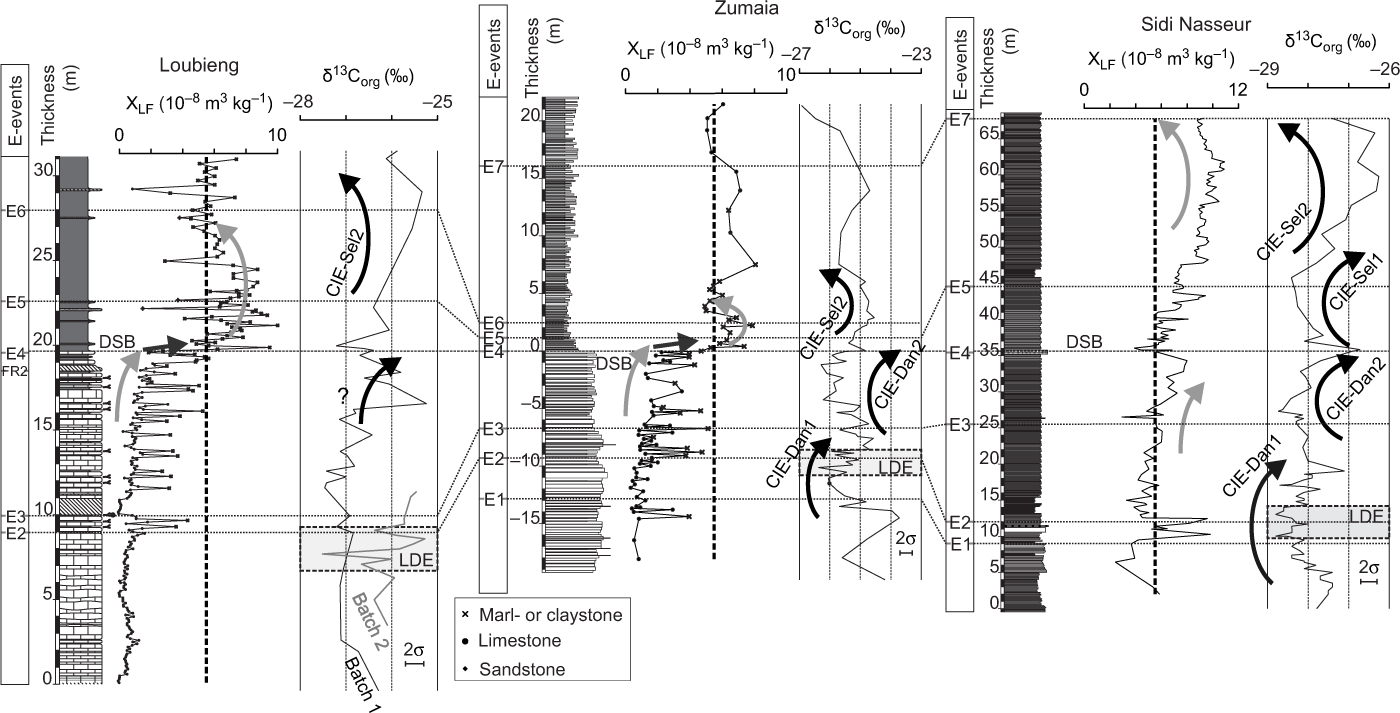
Fig. 3. Comparison between magnetic susceptibility, organic carbon isotopes (δ13Corg) and biostratigraphic E-event results for the Loubieng, Zumaia and Sidi Nasseur sections (partly based on Storme et al. Reference Storme, Steurbaut, Devleeschouwer, Dupuis, Iacumin, Rochez and Yans2014). DSB – Danian–Selandian boundary; LDE – Latest Danian Event; FR2 – second radiation of fasciculiths; E – bio-events.
The present study also pinpoints the second influx of various Lithoptychius species, known as the second Fasciculithus radiation (Bernaola et al. Reference Bernaola, Martín-Rubio and Baceta2009; Schmitz et al. Reference Schmitz, Pujalte, Molina, Monechi, Orue-Etxebarria, Speijer, Alegret, Apellaniz, Arenillas, Aubry, Baceta, Berggren, Bernaola, Caballero, Clemmensen, Dinares-Turell, Dupuis, Heilmann-Clausen, Hilario Orus, Knox, Martin-Rubio, Ortiz, Payros, Petrizzo, von Salis, Sprong, Steurbaut and Thomsen2011) at exactly 18.70 m, between samples 27a (new) and 27b (former sample 27 of Steurbaut & Sztrákos, Reference Steurbaut and Sztrákos2008), respectively.
It should be noted that the position of E2 lacks precision owing to the scarcity of suitable material (clay or marl) in this interval and could be located in the 2 m below. Its position is justified here as it is coherent with what is observed in the Zumaia section.
4.b. Colour
4.b.1. Loubieng
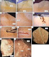
At Loubieng, the sediment colour mostly depends on the lithology. Limestone beds are white (N9), very light grey (N8) or in the majority yellowish grey (5Y 8/1). Marl and claystone ranges from yellowish grey (5Y 8/1) to olive grey (5Y 4/1). However, 54 ‘yellow’ samples and 11 ‘red’ ones break this strict link to lithology: they are encountered as coloured levels whose stratigraphic extent is independent from the limestone and marl beds. Note that the denomination of levels as ‘yellow’ and ‘red’ used generally in this study is based on their hue and their magnetic mineralogy (see Section 4.e) and is not part of the ISCC-NBS classification.
The ‘yellow’ samples have a hue of 10YR in the Munsell system and range from 10YR 8/2 (very pale orange) to 10YR 8/5 (10YR 8/6 being dark yellowish orange). ‘Yellow’ samples have a particularly strong chroma (up to 6 in the chromatic scale) between 7 and 9 m. The ‘yellow’ colour is observed in polished sections as milli- to centimetre-wide bands that are not necessarily parallel (Fig. 4e), overprinting bioturbation (Fig. 4a–d). The colour is sometimes more pronounced near bioturbation (Fig. 4a, c, d). Oxides can be found disseminated in the bulk rock: orange iron oxides and black manganese oxides (Fig. 4f–h). The rock can sometimes be discoloured (Fig. 4h). The ‘red’ samples have a hue of 10R or 5YR. Colours are pale red (10R 6/2) in limestone and range from moderate brown (5YR 4/4) to light brown (5YR 6/4) in marl and claystone. These ‘red’ levels are found between 16 and 20 m. Bioturbation strongly mixes different shades of ‘red’ (arrows in Fig. 4j, k), and near small fractures discolouration can be seen (Fig. 4i).

Fig. 4. (a–d) ‘Yellow’ levels overprinting bioturbation. (e) Non-parallel ‘yellow’ levels. (f–h) Oxide remineralizations and discolouration around these remineralizations (h). (i–k) ‘Red’ samples with strong mixing due to bioturbation, highlighted by several shades of ‘red’ (arrows). Discolouration is also observed in these samples close to a fracture (i).
4.b.2. Zumaia
At Zumaia ‘grey’ and ‘red’ samples can be identified. ‘Grey’ samples display colours from medium grey (N5) to yellowish grey (5Y 8/1). Twenty-three ‘red’ samples have a hue of 5R, 10R or 5YR and colours between greyish red (10R 4/2) and pale red (10R 6/2), or between pale brown (5YR 5/2) and pinkish grey (5YR 8/1). Two ‘yellow’ samples were found, with a hue of 10YR. As in Loubieng, bioturbation is highlighted by colour contrasts.
4.b.3. Sidi Nasseur
The Sidi Nasseur section samples are very monotonous in lithology and colour. They are therefore not characterized by colour any further.
4.c. Magnetic susceptibility
4.c.1. Loubieng
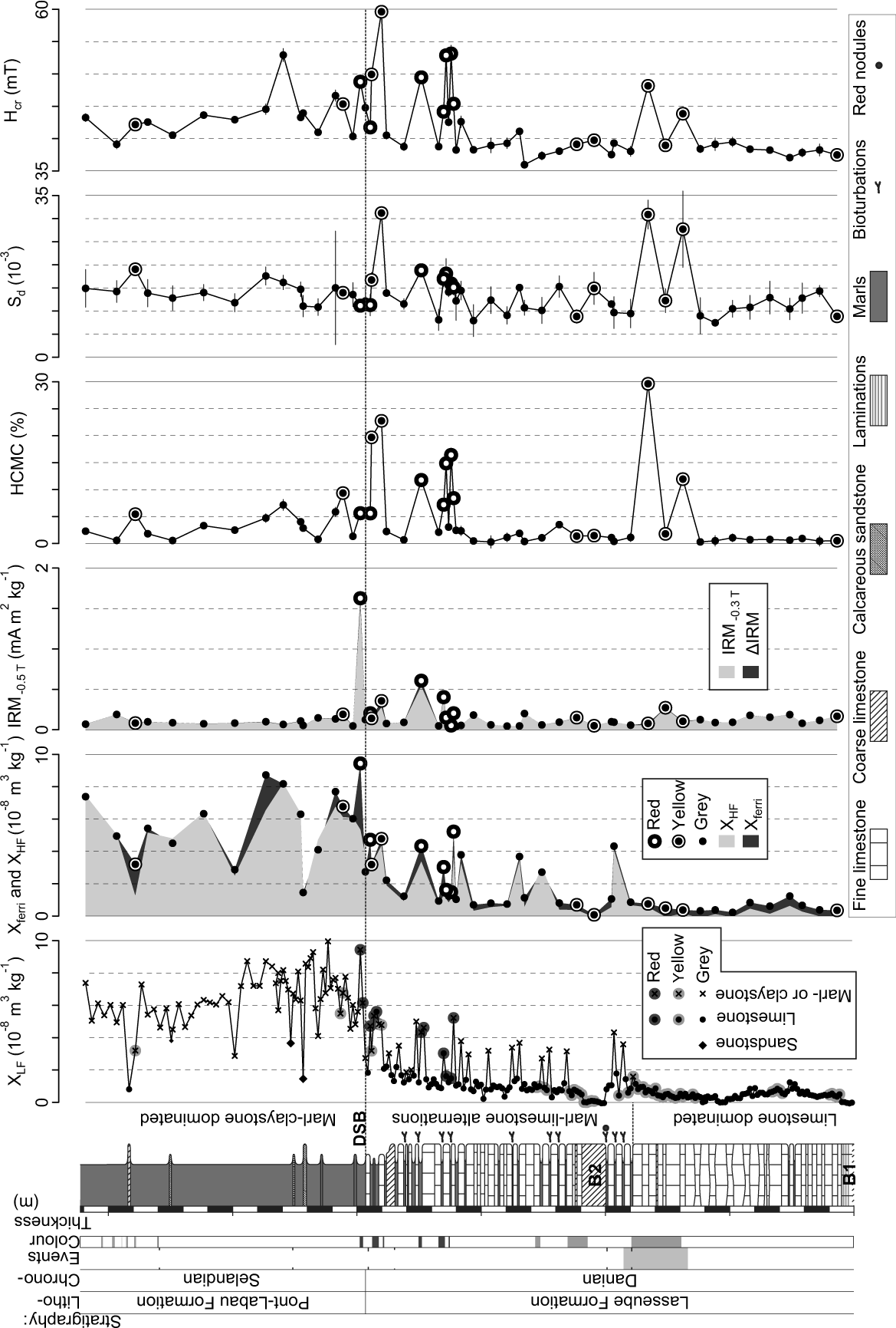
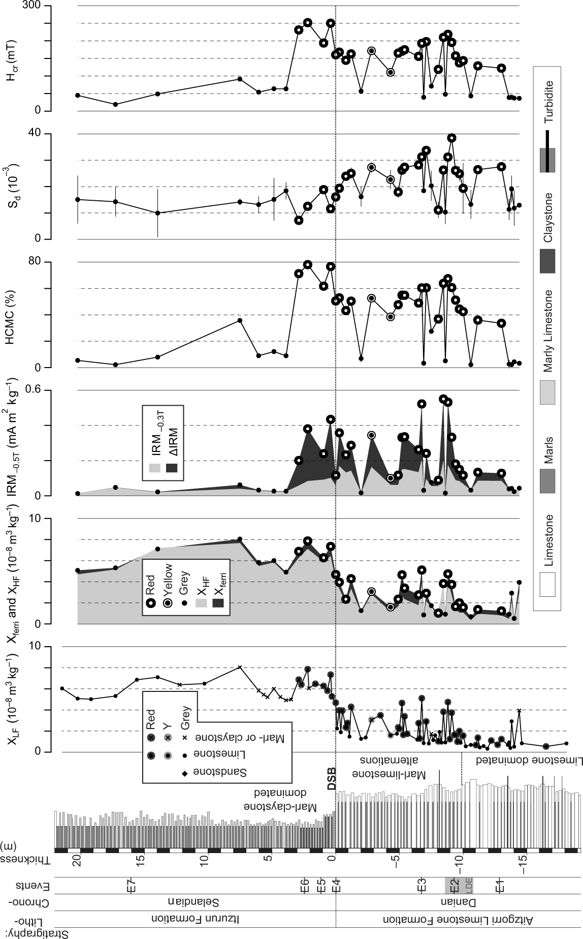
The Loubieng section can be divided into the three following intervals based on lithology and XLF (Fig. 5):
(1) The first interval is dominated by limestone beds from the bottom of the section up to 8.95 m at E2. XLF values are generally under 1 × 10⁻⁸ m3 kg−1. Ferrimagnetic minerals contribute significantly but monotonously to XLF, as the Xferri values can reach up to 0.6 × 10⁻⁸ m3 kg−1 and remain broadly constant. XHF values, representing paramagnetic minerals, vary between c. 1 × 10⁻¹⁰ m3 kg−1 and 0.6 × 10⁻⁸ m3 kg−1. The amplitudes of variations of XHF are much higher than the variations of Xferri; thus, fluctuations in XHF are at the source of the changes in XLF. XHF values gradually reach two local maxima: (i) at 2.5 m, where two marlstone beds intercalate within the limestone beds, and (ii) at 8.95 m, where the onset of marl–limestone alternations mark stronger detrital input (Fig. 5). All these values remain low, implying low contents of paramagnetic and ferromagnetic minerals in this interval.
(2) The second interval is characterized by marl–limestone alternations observed from E2 at 8.95 m to the DSB at 19.70 m. The XLF values generally exceed 3 × 10⁻⁸ m3 kg−1 in marl beds, while they rarely exceed 2 × 10⁻⁸ m3 kg−1 in the limestone beds. However, at the top of this second interval, two ‘red’ limestone samples at 16.5 and 19 m have XLF values higher than 3 × 10⁻⁸ m3 kg−1 and 2 × 10⁻⁸ m3 kg−1, respectively, while two marl samples at c. 18 m have XLF values close to 2 × 10⁻⁸ m3 kg−1. In the two ‘red’ limestone samples, high Xferri values are observed, indicating the presence of ferrimagnetic minerals as the source of the high XLF values. From 15 m to the DSB, the XLF values in the limestone beds generally increase, reflecting the increasing dominance of the detrital input in the sedimentation.
(3) Prevalent marl and claystone characterizes the third interval. Above the DSB, XLF values generally exceed 4 × 10⁻⁸ m3 kg−1, and reach up to 8 × 10⁻⁸ m3 kg−1 in the interval between the DSB and 25 m. Above 25 m, the XLF values decrease and stabilize at c. 6 × 10⁻⁸ m3 kg−1.

Fig. 5. Magnetic parameters for the Loubieng section. The error bar is for 2σ for each measurement. The errors for XLF, XHF and Xferri are not provided but are typically smaller than the symbols. If the error bar is absent for all other parameters it means the error is smaller than the symbols. See Table 1 for further details on the isotopic data. R – red; Y – yellow.
Beyond these broad trends, distinct beds show particularly low XLF values. These beds are:
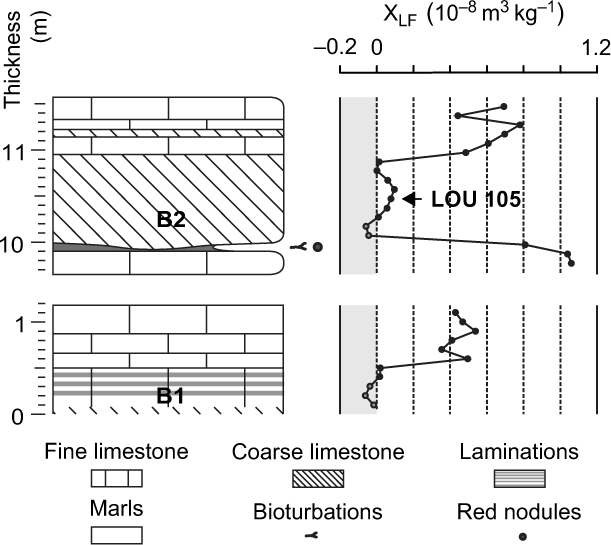
(1) Massive limestone beds having XLF values ranging from −0.1 to 0.1 × 10⁻⁸ m3 kg−1 and marked by particularly low values at their bottoms. Two of these limestone beds are found from 0 to 0.6 m and from 10 to 11 m (B1 and B2; Figs 5, 6). Additionally, limestone beds are found with XLF values lower than 0.1 × 10⁻⁸ m3 kg−1 from 4 to 7 m, within an interval where lenticular bedding is observed.
(2) Sandstone and limestone beds in the Selandian part of the section with XLF values below or c. 4 × 10⁻⁸ m3 kg−1. They crop out in the field as more indurated beds within the softer marl and claystone dominating in that interval.

Fig. 6. Close-up view of magnetic susceptibility in beds B1 and B2 of the Loubieng section.
4.c.2. Zumaia
Based on lithology and XLF, the Zumaia section can be divided into three intervals (Fig. 7):
(1) A limestone-dominated interval from the bottom of the section (−18 m) to −10 m, which mainly displays low XLF values of c. 1 × 10⁻⁸ m3 kg−1. Thin marl layers were observed, but the large sampling interval did not allow their detailed study.
(2) An interval of marl–limestone alternations, from −10 m up to the DSB at 0 m. Marl samples generally have higher XLF values (more than 2 × 10⁻⁸ m3 kg−1) than the limestone ones (XLF values c. 2 × 10⁻⁸ m3 kg−1). Two marl samples have, however, lower XLF values than the average limestone at −7.5 and −5 m, and three limestone samples have higher XLF than the average marl at −7, −6.5 and −3.5 m. From −12 m (in the first interval) to the DSB, the limestone XLF values tend to increase progressively from 1.5 × 10⁻⁸ m3 kg−1 to 2 × 10⁻⁸ m3 kg−1, indicating an upward increase in the detrital fraction in the sediment.
(3) Above the DSB, XLF values suddenly increase to c. 6 × 10⁻⁸ m3 kg−1 in an interval with a more important terrigenous component. These values are far above the values observed in the Danian. A maximum value of c. 8 × 10⁻⁸ m3 kg−1 is reached right above the DSB. The XLF values then decrease to 5 × 10⁻⁸ m3 kg−1 at 4 m, and increase again to 8 × 10⁻⁸ m3 kg−1 at 8 m. After these rapid fluctuations, the XLF values gently decrease to 6 × 10⁻⁸ m3 kg−1 at the top of the section.

Fig. 7. Magnetic parameters for the Zumaia section. The error bar is for 2σ. The errors for XLF, XHF and Xferri are not provided but are typically smaller than the symbols. If the error bar is absent for all other parameters it means the error is smaller than the symbols. The log was taken from Storme et al. (Reference Storme, Steurbaut, Devleeschouwer, Dupuis, Iacumin, Rochez and Yans2014); see Table 1 for further details on the isotopic data.
Generally, XHF is higher than Xferri, so that XLF mainly reflects a paramagnetic signal. However, 12 ‘red’ samples are characterized by Xferri values higher than their XHF. The high Xferri values in these samples indicate the presence of ferrimagnetic minerals, and raises the XLF above the values expected for the respective lithologies.
4.c.3. Sidi Nasseur
The Sidi Nasseur section displays a smooth, long-term trend in increasing XLF values from the bottom of the section (XLF c. 5 × 10⁻⁸ m3 kg−1) to the DSB, overlain by minor fluctuations (Fig. 8). Through the DSB the values locally decrease with an amplitude of 4 × 10⁻⁸ m3 kg−1 and then continue to increase. This increase in XLF values reaches a maximum of 11 × 10−8 m3 kg−1 at 62 m, followed by a smooth decrease of XLF values until the end of the section (down to 9 × 10⁻⁸ m3 kg−1). XLF is mainly influenced by paramagnetic minerals, as revealed by the low values of Xferri. However, abnormally high values of XLF are observed at c. 10 and 12 m, in an interval around E2 affected, among other things, by the presence of glauconitic beds.
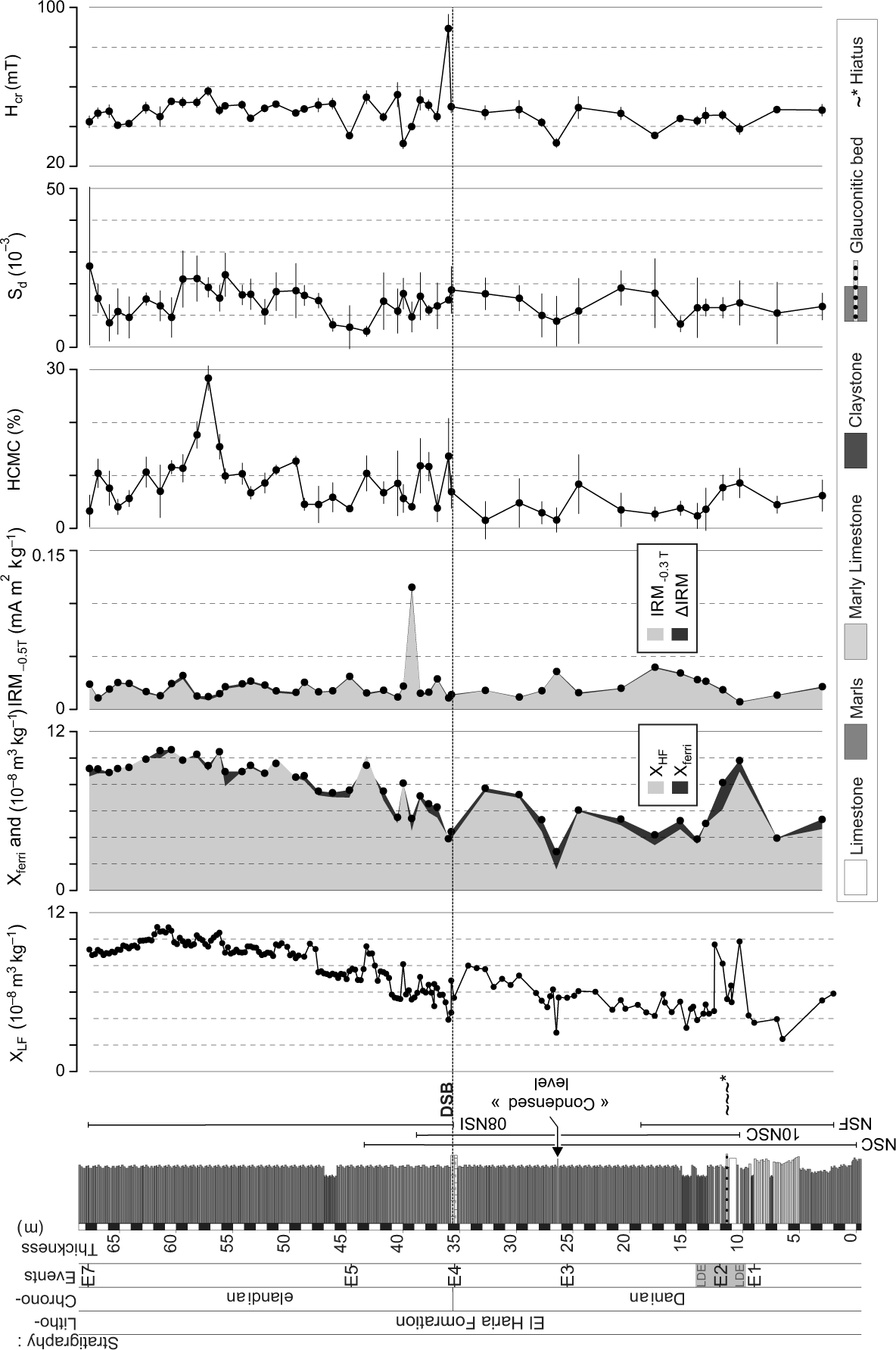
Fig. 8. Magnetic parameters for the Sidi Nasseur section. The error bar is for 2σ. The errors for XLF, XHF and Xferri are not provided but are typically smaller than the symbols. If the error bar is absent for all other parameters it means the error is smaller than the symbols. The log comes from Storme et al. (Reference Storme, Steurbaut, Devleeschouwer, Dupuis, Iacumin, Rochez and Yans2014); see Table 1 for further details on the isotopic data. The position of the subsections making up the composite sections (NSF, NSC, 08NSI, 10NSC) is also provided (at the right of the litholog).
4.d. J-meter magnetic parameters
4.d.1. Loubieng
The results of the magnetic parameters measured in Loubieng are shown in Figure 5. The IRM−0.5 T is commonly lower than 0.25 mA m2 kg−1 throughout the section. However, higher IRM−0.5 T values are found in ‘yellow’ and ‘red’ samples. Decomposition of the IRM−0.5 T into ferrimagnetic (IRM−0.3 T) and high-coercivity contributions (ΔIRM) shows that these samples have low ΔIRM values. This implies that the high IRM−0.5 T values (i.e. the magnetization at −0.5 T) come from a relatively important low-coercivity mineral content (e.g. magnetite) rather than only from haematite or goethite as the colour would suggest. High IRM peaks associated with ‘red’ samples are related to high Xferri values, ranging from 0.4 to 4 × 10⁻⁸ m3 kg−1, further confirming the importance of low-coercivity minerals. High HCMC and Hcr values (up to 30 % for HCMC) in ‘red’ and ‘yellow’ samples nonetheless suggest the presence of high-coercivity minerals, such as haematite and goethite. High Sd values (between 20 × 10−3 and 35 × 10−3) are found only in ‘yellow’ samples, indicating a viscous behaviour.
Other samples at 21 and 24 m display high Xferri values. As only a small part of the sample used to measure XLF was measured in the J-meter for XHF, these high Xferri values could be due to sample heterogeneity, and are thus regarded here as non-significant. High Hcr values are observed in a sample at 23 m. No other magnetic parameter follows this behaviour in this sample, and it does not display a ‘red’ or ‘yellow’ colour. This high Hcr value at 23 m is thus deemed non-significant, too.
4.d.2. Zumaia
The results of the magnetic parameters of Zumaia are shown in Figure 7. The high-coercivity mineral contribution (ΔIRM) accounts for more than 50 % of IRM−0.5 T, suggesting that the IRM−0.5 T values of the ‘red’ samples in Zumaia are strongly influenced by high-coercivity minerals. This is confirmed by the HCMC values for these samples ranging from 25 % to nearly 80 %. IRM−0.5 T and Hcr correlate very well with HCMC (r = 0.84 and r = 0.98, respectively).
Sd and HCMC follow similar trends in the Danian part of the section, while their trends diverge above the DSB. In the Danian, samples with high Hcr and HCMC are linked with the highest Sd values: up to 30 × 10−3. But in the Selandian, where the highest Hcr and HCMC values in the section are found, the Sd values are systematically lower than 20 × 10−3. As Sd is a parameter related to the size of the ferromagnetic minerals contributing the most to magnetization, this indicates that the size populations of the high-coercivity minerals are strongly distinct between the Danian and Selandian ‘red’ samples.
4.d.3. Sidi Nasseur
Magnetic parameters measured in Sidi Nasseur (Fig. 8) rarely exceed the background values. The Sd values display no specific trend considering the high analytical error. Isolated high values in IRM−0.5 T, Hcr or HCMC can be observed. However, in this section these three parameters are inconsistent with each other. Therefore, a broad magnetic mineralogical trend can barely be deduced. The influence of high-coercivity minerals seems very faint, as shown by the IRM−0.5 T curve where mainly low-coercivity minerals contribute to the signal (the ΔIRM is negligible).
4.d.4. Comparison of the sections in the Day Plot
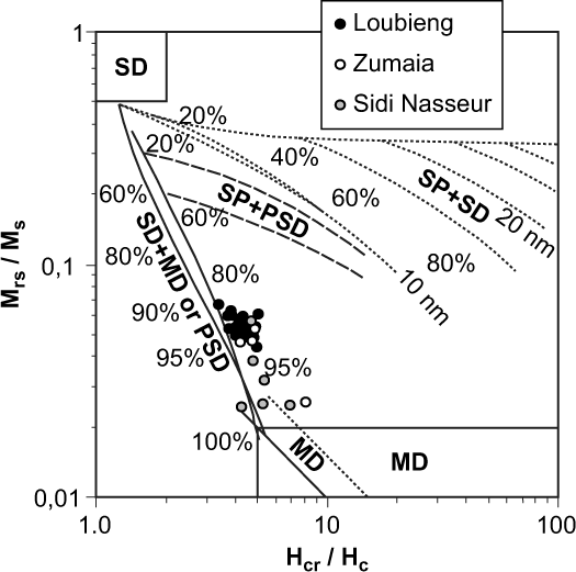
The samples of all three sections saturated at or below 0.5 T display pseudo-single domain (PSD) behaviour in the Day diagram (Fig. 9). Following Dunlop (Reference Dunlop2002), this could be attributed either to PSD-sized grains or to a mixture of grains that are between SD and MD size. Thus, the size of the low-coercivity minerals cannot be precisely determined. Roberts et al. (Reference Roberts, Tauxe, Heslop, Zhao and Jiang2018) suggested that the Day diagram is ambiguous for domain state diagnosis, making its interpretation more difficult. More generally, these samples do not display signs of significant SP behaviour in the Day diagram. Loubieng and Zumaia samples show similar values, whereas Sidi Nasseur samples plot closer to the ‘MD’ field as defined by Dunlop (Reference Dunlop2002).

Fig. 9. Day plot for Loubieng, Zumaia and Sidi Nasseur samples with HCMC < 5 %, which excludes ‘yellow’ and ‘red’ samples, because of their high-coercivity mineral contribution making a high-field slope correction meaningless. The mixing lines are redrawn from Dunlop (Reference Dunlop2002). SD – single domain; PSD – pseudo-single domain; MD – multidomain; SP – superparamagnetic.
4.e. Additional magnetic analyses with the MPMS 3 instrument
4.e.1. Loubieng
The dominance of goethite or haematite in the magnetic behaviour were established with the additional magnetic analyses performed with the MPMS 3 instrument, which then determined the choice of the hue values used to discriminate ‘yellow’ and ‘red’ samples. The results are summarized in Table 2, and shown for representative samples in Figure 2. The saturation field, i.e. the field above which the Mrh is constant, is deduced from the hysteresis loop at 7 T. The saturation field above 6 T of some samples is linked to the presence of goethite, as it is the only common natural magnetic mineral not saturated above 5 T (Dekkers, Reference Dekkers, Gubbins and Herrero-Bervera2007). In all these goethite-bearing samples, an unblocking temperature lower than 80 °C is observed. We thus consider that a linear regression of the IRM against temperature, at temperatures over 80 °C, fits the behaviour of other magnetic minerals at lower temperatures. This in turn allows us to calculate GC (see Section 3.d.7). The GC values in the goethite-bearing samples range between 20 and 100 %. The other samples have zero GC values and saturation magnetic fields between 2 and 4 T, which are compatible with haematite (Dekkers, Reference Dekkers, Gubbins and Herrero-Bervera2007). At low temperatures, a small fluctuation is observed in nearly all samples in the cooling curve at c. −25 °C. This is interpreted as the Morin transition, a haematite magnetic phase transition that occurs below −12 °C (Özdemir et al. Reference Özdemir, Dunlop and Berquó2008). The temperature of this transition can be lowered in low grain-sized haematite (to −23 °C for c. 0.1 µm grains, but dramatically lower for increasingly lower sizes) or with cation substitution (1 % Ti substitution suppressing the Morin transition below 10 K), and is further dependent on lattice defects, pressure and applied field (Bowles et al. Reference Bowles, Jackson and Banerjee2010). The Morin transition is, however, not observed in sample LOU084. This could be explained either by the absence of haematite (with goethite as the only high-coercivity mineral in that sample) or by lowering of the temperature of the Morin transition (for instance owing to cation substitution or low grain size; Bowles et al. Reference Bowles, Jackson and Banerjee2010). However, the first explanation is here preferred, as the GC value is 100 %. Based on the saturation field and the GC parameter, it is possible to determine which high-coercivity mineral dominates the signal in each sample. The effect on the sample’s hue is clear: the dominance of goethite (or more precisely a GC value above 40 %) coincides with a hue of 10YR, while the colour of more reddish samples coincides with the dominance of haematite (GC ≤ 20 %).
Table 2. Summary of the additional MPMS 3 magnetic analyses results and comparison with colour and J-meter magnetic parameters (HCMC, Hcr and Sd) for the Loubieng section
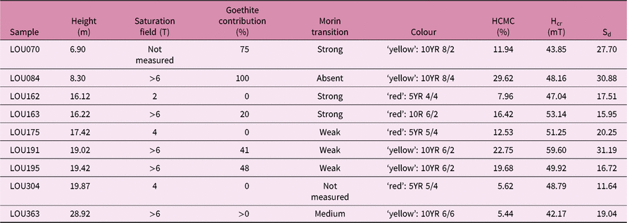
The analyses of three samples are compared in Figure 2. The displayed samples show the presence of high-coercivity minerals: haematite (LOU162), a mix of haematite and goethite (LOU195) and goethite (LOU084). Sample LOU084 displays a perfect reversibility of the remanent magnetization against temperature during cooling, which is not the case when haematite is present. It also shows an increasing slope of the IRM against the magnetic field at 0.3 T, indicating the presence of a magnetic mineral with higher coercivity than in LOU162 and LOU195.
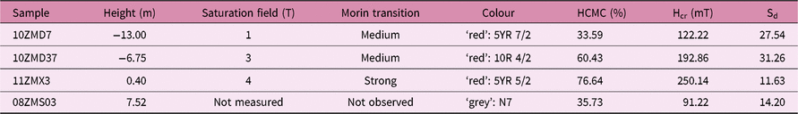
4.e.2. Zumaia
Additional magnetic analyses were performed on four samples at Zumaia. The results are shown in Table 3. For three ‘red’ samples, the ‘room-temperature’ hysteresis loops and IRM against temperature data, respectively, reveal saturation fields of between 1 and 4 T and the presence of the Morin transition between −74 and −33 °C. The presence of haematite in these three ‘red’ samples is thus confirmed and linked to their colour. A fourth ‘grey’ sample, 08ZMS03, which has a HCMC of 35 %, does not display the Morin transition. The saturation field of this sample could not be determined with certainty because of its weak magnetization that was at the source of a low S/N ratio.
Table 3. Summary of the additional MPMS 3 magnetic analyses results and comparison with colour and J-meter magnetic parameters (HCMC, Hcr and Sd) for the Zumaia section
4.e.3. Sidi Nasseur
Sidi Nasseur is not studied using the MPMS 3 because of the absence of evidence for high-coercivity minerals.
4.f. Organic carbon isotopes (δ13Corg)
The δ13Corg values dataset is provided in Tables S1–S6 in the online Supplementary Material.
4.f.1. Sidi Nasseur
The δ13Corg trends at Sidi Nasseur are divided into four large-scale carbon isotopic excursions (CIEs): CIE-Dan1, CIE-Dan2, CIE-Sel1 and CIE-Sel2 (Fig. 3). These CIEs were first defined in Sidi Nasseur, where they are the most clearly expressed, and then correlated to Zumaia and Loubieng. In Sidi Nasseur, the onset of CIE-Dan1 is at 3 m, with δ13Corg values at c. −27.4 ‰. These values decrease to −28.8 ‰ at 10 m, and then increase to reach values stabilizing at c. −28.0 ‰ at 23 m, defining the end of CIE-Dan1. In CIE-Dan2, starting at 23 m, the δ13Corg values first decrease to −28.7 ‰ at 27 m and then increase to −26.7 ‰ at 36 m, above the DSB. A series of negative shifts of −1 ‰ are documented in the Danian at 10, 13, 17 and 27 m. A third negative CIE starts from the DSB and goes up to 50 m, where an inflection point changes the curvature, starting the positive CIE-Sel2. The trend made by the successive sequences of CIE-Sel1 and 2 starts with a decrease in δ13Corg values from −26.7 ‰ at 36 m to a minimum of −28.4 ‰ at 46 m, followed by an increase to reach a maximum of −26.3 ‰ between 55 and 60 m. Values then decrease to −27.4 ‰ at the top of the series.
4.f.2. Zumaia
The δ13Corg values in Zumaia (Fig. 3) start at −24.2 ‰ at the bottom of the section, decrease to −25.6 ‰ at −18 m, and increase again up to −23.7 ‰ at −14 m. From −14 m up to the DSB, the δ13Corg series shows two large negative CIEs. CIE-Dan1 is found between −14 and −8 m, and is distinguished by δ13Corg values which decrease from −23.7 ‰ to a minimum of −26.4 ‰ at −10 m and increase to −24.6 ‰ at −8 m. CIE-Dan2, found between −8 m and the DSB, is marked by δ13Corg values that start at −24.6 ‰ at −8 m, decrease to −26.2 ‰ between −5 and −1 m, and then increase to −25.5 ‰ right below the DSB. In CIE-Dan1 and 2, smaller negative shifts are observed with an amplitude of −1 ‰ or more between −10 and −7 m. Above the DSB, we attribute CIE-Sel2 to an increase in δ13Corg values from −25.5 ‰ to −24.6 ‰ at 3 m and a decrease down to −25.7 ‰ at 7.5 m. After 7.5 m, the δ13Corg values increase to −24.7 ‰ at 14 m and decrease to −26.9 ‰ at the top of the section.
4.f.3. Loubieng
The isotopic geochemistry of the Loubieng section was studied in two batches of samples (Fig. 3). The δ13Corg values of batch 1 decrease from −26.3 ‰ at the bottom of the section to −27.1 ‰ at 2.5 m. The values then tend to stabilize at c. −27 ‰ up to 16 m. The δ13Corg values tend to increase from −26.8 ‰ at 16 m to −25.8 ‰ at 18.5 m. Just below the DSB, values decrease back to c. −26.6 ‰, which is the mean value going through the boundary. In the Selandian, CIE-DS1 is hinted at by a few samples: δ13Corg values increase from −27.2 ‰ to −25.3 ‰, and then undergo a decrease of 0.6 ‰ at the end of the section.
The δ13Corg values for batch 2 tend to increase from −26.1 ‰ at 3 m to −25.5 ‰ at 12 m (Fig. 3). Small-scale shifts are found at 7 m with an amplitude of −1.5 ‰, at 8.5 m with a positive shift of 2.2 ‰ and at 9 m with a negative shift of −1.1 ‰
4.f.4. General stratigraphic framework
A general chemostratigraphic framework was established from the correlation of the different CIEs, which was based on the biostratigraphic E-events (Fig. 3). Nonetheless, the position of E7 is in conflict with CIE-Sel2 in Zumaia and Sidi Nasseur. Apart from this problem, the CIEs are well correlated between the three sections.
The LDE isotopic anomaly should be coeval with bio-event E2, marking the P3a/P3b boundary (Bornemann et al. Reference Bornemann, Schulte, Sprong, Steurbaut, Youssef and Speijer2009). Based on this bio-event E2, small-scale δ13Corg negative shifts can be attributed to the LDE (at c. 7 m in Loubieng, c. −9 m in Zumaia and c. 11 m in Sidi Nasseur; Fig. 3). These shifts are found in the larger δ13Corg trend made by CIE-Dan1. In all three sections, we associate the LDE with two successive δ13Corg negative excursions rather than only one (Fig. 3), in agreement with observations reported in other sections (Deprez et al. Reference Deprez, Jehle, Bornemann and Speijer2017). It should be noted that similar δ13Corg negative shifts can be found in other intervals of the studied sections.
5. Discussion
5.a. Geological meaning of the magnetic parameters
5.a.1. Magnetic susceptibility
In Loubieng and Zumaia, MS generally follows the lithological changes (Figs 5, 7) and XLF usually reflects XHF. This implies that the XLF changes throughout the sections can be mainly explained by variations in paramagnetic mineral content, such as clays, throughout the section. Nonetheless, high Xferri values in certain samples indicate the locally important influence of ferrimagnetic minerals on XLF. These minerals strongly increase XLF, independently from lithology. At Loubieng and Zumaia, XLF can thus be used as a proxy for paramagnetic minerals and terrigenous input, provided that Xferri is low and that XLF follows the lithological changes. This impacts any high-resolution analysis of MS results, which should be constrained by sample-by-sample lithological observations.
At Sidi Nasseur, ferromagnetic minerals have no significant effect on the XLF, as suggested by the lack of consistency between the magnetic parameters and low values in Xferri and ΔIRM. Thus, paramagnetic minerals control the XLF signal in Sidi Nasseur, which can be reliably used as a proxy for terrigenous input. However, high XLF values during the LDE could be due to the presence of localized glauconitic beds, and may therefore not be used to follow detrital changes in this interval.
The ‘red’ levels in Loubieng can be found in combination with relatively high concentrations of low-coercivity minerals, as indicated by the high values in IRM−0.3 T and Xferri (Fig. 4). This can be interpreted as a simultaneous input of low- and high-coercivity minerals, or as the oxidation of primary low-coercivity minerals to haematite. Regardless of the interpretation, ‘red’ beds can indicate the presence of ferromagnetic minerals in sufficient amounts to affect the MS signal. This further highlights the need to check each sample for lithology and colour variations when interpreting XLF as a proxy for paramagnetic minerals.
5.a.2. J-meter magnetic parameters
In the Loubieng and Zumaia sections, the J-meter magnetic parameters show a consistent link to colour. Coloured samples in both sections have high values of HCMC and Hcr, two parameters related to the presence of high-coercivity minerals. At Zumaia, coloured samples even have high ΔIRM values, indicating that a significant part of the magnetization is due to these high-coercivity minerals. This link between magnetic parameters and colour thus suggests that high-coercivity minerals are at the origins of the observed colours. The proxy for viscous decay of magnetization, Sd, shows high values in specific coloured samples only (see Sections 5.b and 5.c). In given intervals, HCMC, Hcr and Sd show similar trends in similar samples (i.e. having the same colour). This indicates that these parameters are all controlled by one population of magnetic minerals at a time.
All ‘red’ and ‘yellow’ samples selected for analysis with the MPMS 3 display conclusive evidence for the presence of haematite and/or goethite in Loubieng and Zumaia. In addition, goethite dominates in ‘yellow’ levels (hue of 10YR) and haematite in ‘red’ ones (hue of 10R and 5YR). Thus, a simple comparison to a colour chart could be used to identify these two minerals and estimate their relative proportions. The magnetic parameters obtained for these samples with the J-meter also indicate the presence of these high-coercivity minerals. HCMC can be used to detect high-coercivity minerals when it is higher than the background, even with relatively low values (just above 5 %; see samples LOU304 and LOU363 in Table 2). However, it should be kept in mind that this parameter is a ratio, for which high values can arise simply from analytical variability. Therefore, high values in HCMC, e.g. 35 % for the ‘grey’ sample 08ZMS03 (Table 3), must be regarded with caution in very weakly magnetic samples to avoid false positives. Furthermore, seemingly significant values of Hcr, IRM−0.5 T, or Xferri in certain samples lack further evidence of ferromagnetic mineral presence. In these cases the parameters cannot be interpreted meaningfully. And in some cases, the strong analytical variability of the parameters entirely prevents interpretation of any fluctuation (such as for Sd in Sidi Nasseur; Fig. 8).
5.b. Coloured levels in Loubieng
The particularly strong ‘yellow’ colours (10YR) overprint the bioturbation features (Fig. 4a–d), implying a post-depositional origin. In addition, the viscous behaviour of these ‘yellow’ levels is significantly higher than in the surrounding samples (Sd > 20 × 10−3). A link between post-depositional formation and viscous behaviour is therefore suggested for goethite in this section. A comparable link between chemical remagnetization (i.e. remagnetization through the formation of post-depositional minerals) and magnetic behaviour attributable to low grain size has already been noted several times in the past in carbonate rocks (e.g. Jackson & Swanson-Hysell, Reference Jackson, Swanson-Hysell, Elmore, Muxworthy, Aldana and Mena2012). For instance the Morin transition could not be observed in secondary haematite from fracture and fault zones (Zwing et al. Reference Zwing, Matzka, Bachtadse and Soffel2005). This could be due to low grain size, which would lower the Morin temperature and prevent its detection in the tested temperature ranges. Nonetheless, other processes could also explain this, such as cation substitution in the haematite (Bowles et al. Reference Bowles, Jackson and Banerjee2010). Authigenic magnetite in remagnetized limestones is also known to have viscous or SP behaviour (Jackson & Swanson-Hysell, Reference Jackson, Swanson-Hysell, Elmore, Muxworthy, Aldana and Mena2012).
The colour distribution, and the distribution of the haematite pigment of the ‘red’ levels of Loubieng, is affected by bioturbation (cf. Section 4.b.1). Primary haematite as well as very early diagenetic haematite could have been added in the recently deposited sediment and then have been mixed by burrowing benthic organisms, giving the colour distributions observed in the polished sections. However, bioturbation can change the porosity, oxygen concentration and organic matter content in the sediment. The physical difference between the bioturbated and non-bioturbated sediment could, therefore, also affect the distribution of haematite that would form after bioturbation, at least before cementation impeded the mobility of the ions needed to form the oxides. Low organic matter content in the Loubieng section (S. Wouters, unpub. M.Sc. thesis, Université Libre de Bruxelles, 2016) is consistent with oxic conditions allowing haematite formation. Nonetheless, this does not necessarily imply an authigenic origin of this haematite. More importantly, we observe no consistency in the way bioturbation affects colour: the bioturbation features are neither systematically redder than the surrounding sediments nor systematically less red. Both cases can be observed (arrows in Fig. 4j, k). This behaviour is most easily explained by the bioturbation of sediments that already have different concentrations of red pigment. A very late diagenetic origin seems thus less probable.
5.c. Coloured levels in Zumaia
The ‘red’ levels of Zumaia can be divided in two groups, Danian and Selandian, based on the Sd parameter. Danian ‘red’ levels have Sd values mostly above 20 × 10−3, while Selandian ‘red’ levels have Sd values lower than 20 × 10−3. This threshold is identical to the one chosen in Loubieng. As both groups have samples with high HCMC, this difference is not explained by the dilution of the magnetic signal of haematite by another magnetic mineral. Conversely, the origin of haematite could be different between the Danian and the Selandian. A hypothesis could be that the Danian haematite is of post-depositional origin. Dinarès-Turell et al. (Reference Dinarès-Turell, Stoykova, Baceta, Ivanov and Pujalte2010) formulated an early diagenetic origin for the fine and pigmentary haematite in these levels. On the other hand, the Selandian haematite could be at least partly primary, and made of coarser grains than in the Danian. This would imply a relationship between the grain size, viscous behaviour and diagenetic origin of a magnetic mineral, in this case haematite. This hypothesis could explain why ‘red’ levels in Loubieng are observed only near the DSB while in Zumaia they are found much earlier. Primary haematite would have been deposited around the DSB in both sections, and haematite in the Danian beds of Zumaia would have formed after sedimentation by diagenetic processes. That would thus imply a primary origin for the haematite at Loubieng. However, this cannot be confirmed by the Sd parameter in Loubieng, as the HCMC is low, which implies that the Sd parameter is related to low-coercivity minerals.
5.d. Gravitational deposits in Loubieng
At Loubieng, event deposits display abnormally low XLF values compared to the other beds of the series (Fig. 5). In the Danian, these are the metric B1 and B2 beds and two thinner beds at 5.2 and 6 m in the zone where beds are lenticular. These limestone beds have a different microfacies than the surrounding limestone beds. Their microfacies are bioclastic packstones containing micritic clasts and bioclasts having clear neritic origins (like red algae), while the other limestone beds consist of planktonic Globigerina and Globotruncana mudstones to wackestones, indicating a more pelagic setting (S. Wouters, unpub. M.Sc. thesis, Université Libre de Bruxelles, 2016). A close-up view of the MS values in B1 and B2 (Fig. 6) shows negative XLF values at the bottom of both beds. This indicates a magnetic behaviour dominated by diamagnetic minerals and thus a very low concentration of paramagnetic (usually clays) and ferromagnetic minerals. The sample LOU105, which was taken in B2 and measured using the J-meter, has an XHF of −8 × 10⁻¹⁰ m3 kg−1 and a XLF of 8 × 10⁻¹⁰ m3 kg-1. These data indicate the presence of mainly diamagnetic (carbonates) and ferrimagnetic minerals, and the absence of a significant clay contribution to the signal. The HCMC is 1.5 %, confirming that low-coercivity minerals are the main ferromagnetic minerals in that sample. In B2, the highest MS values are found in the centre of the bed. Altogether this would imply that ferrimagnetic minerals are concentrated there. This argument, combined with the presence of an erosive surface at the bottom of the bed and a microfacies typical of a shallow water carbonate platform environment, indicates that these beds are the record of gravitational deposits which had enough velocity to erode underlying sediments and have a size-dependent redistribution of the minerals within the bed. This latter effect would be responsible for the distribution of low-coercivity minerals in the centre of the bed. The two thin lenticular beds found at 5.2 and 6 m were previously identified as slumps (Peybernès et al. Reference Peybernès, Fondecave-Wallez, Hottinger, Eichène and Segonzac2000; Rocher et al. Reference Rocher, Lacombe, Angelier, Deffontaines and Verdier2000), but facies and low XLF values also suggest that these beds are energetic gravitational deposits as well, bringing proximal material from the shallow water platform into the deep basinal setting of Loubieng.
In the Selandian, a few sandstone and red algae limestone beds (S. Wouters, unpub. M.Sc. thesis, Université Libre de Bruxelles, 2016) display low MS values. Again, these are attributed to gravitational deposits as they are made of material allochthonous to the pelagic setting of Loubieng.
5.e. Depositional changes during the Danian–Selandian transition
Dinarès-Turell et al. (Reference Dinarès-Turell, Stoykova, Baceta, Ivanov and Pujalte2010) ascribed the marl–limestone couplets in Loubieng to precession cycles. Such lithological alternations in other sections have already been attributed to cyclic climate changes where marl beds were deposited under tropical humid conditions and limestone beds under semi-arid conditions (Mutterlose & Ruffell, Reference Mutterlose and Ruffell1999; Moiroud et al. Reference Moiroud, Martinez, Deconinck, Monna, Pellenard, Riquier and Company2012). This implies that the XLF signal, which mainly follows the expression of these alternations, would be linked to climate. At a larger scale, and still based on MS, the section is divided into three intervals. The interval boundaries are at the E2 and E4 bio-events (Fig. 3), and are linked to the LDE and the DSB, respectively. They both mark sudden increases in detrital input. A more gradual increase in detrital input can be observed in Loubieng before E2 and E4 by the increase in XLF in the limestones (at c. 8 m and c. 19 m; Fig. 3).
The marl–limestone alternations at Zumaia are also attributed to precession cycles (Dinarès-Turell et al. Reference Dinarès-Turell, Stoykova, Baceta, Ivanov and Pujalte2010). The lithological contrast is expressed in the XLF signal, suggesting a similar link between climate and XLF as in Loubieng. Also as in Loubieng, the Zumaia section can be divided into three intervals using the bio-events E2 and E4 as boundaries (Fig. 7). A smooth increase in the XLF values in the limestone beds before the DSB is observed, followed by a stronger increase right at the DSB.
Sidi Nasseur shows monotonous XLF characteristics. Hence, clear precession-scale alternations such as those found in Loubieng and Zumaia cannot be clearly observed with our sampling rate. This implies that the XLF signal acquired for Sidi Nasseur can only be used to study long-term effects. These long-terms effects could be related to the E2 and E4 events, but as their expression is different than in Loubieng and Zumaia, and are less clearly expressed, this interpretation would be subject to caution.
The three sections all display a long-term increase in terrigenous input from the upper Danian part of the series to the DSB. At Loubieng and Zumaia, the same abrupt XLF increase is observed at the DSB, while in Sidi Nasseur this increase is gentler, indicating a discrepancy between the Atlantic and Tethyan sections. Still, the long-term increase in terrigenous input throughout the studied interval, observed by the XLF fluctuations and found consistently in all three sections, allows XLF to be used for large-scale correlations.
A discrepancy between the Atlantic and Tethyan sections is put forward by the fact that the CIE-Sel1 δ13Corg trend found in Sidi Nasseur is not clearly observed in Loubieng and Zumaia. This CIE is hinted at between E4 and E5 in Zumaia, but would be concentrated in 1 m of sediments. This points towards low sedimentation rates after the DSB in Loubieng and Zumaia, relative to the other parts of the sections.
In CIE-Sel2, the XLF values follow a similar trend in all three sections, with an increasing and then decreasing trend. These particular trends are concentrated in 3 m in Zumaia, while covering more than 7 m in Loubieng and more than 20 m in Sidi Nasseur. This indicates that Zumaia has a more condensed nature than the other sections in this interval. This is confirmed by the results of Storme et al. (Reference Storme, Steurbaut, Devleeschouwer, Dupuis, Iacumin, Rochez and Yans2014), which showed that the CIE-Sel2 event itself constitutes 6 m in Zumaia, while it encompasses more than 11 m in Loubieng and more than 23 m in Sidi Nasseur. The low sedimentation rate in the basal Selandian observed in the Zumaia section is confirmed by biostratigraphy, with the E-events E4, E5 and E6 following each other in a small interval at the bottom of the Selandian at Zumaia.
The hyperthermal event of c. 30 kyr at the very beginning of the Selandian proposed by Storme et al. (Reference Storme, Steurbaut, Devleeschouwer, Dupuis, Iacumin, Rochez and Yans2014) occurs during a haematite influx event observed in Loubieng and Zumaia. This influx could be due to dry climatic conditions in the gulf of the Biscay area, leading to the formation of haematite in soils. However, the red levels in Zumaia and Loubieng do not correlate clearly, as the primary haematite is found only in the Selandian of Zumaia, whereas it can also be found below the DSB in Loubieng. Furthermore, primary haematite can also originate from the mechanical erosion of haematite-bearing deposits that would have formed earlier. Therefore, a tectonic effect exposing such deposits could equally explain this primary haematite.
Most strikingly, in Loubieng, the start of the gradual increase in XLF before E2 is synchronous with the start of the LDE as we define it based on carbon isotopes, and the start of the gradual increase in XLF before the DSB is synchronous with the first occurrence of the primary red layers. This implies that the increase in lithogenic input is directly related to the suggested climatic events.
6. Conclusions
Magnetic susceptibility data reveals similar patterns or trends in the three sections: patterns linked to a precession-related climatic effect that creates marl–limestone alternations in Loubieng and Zumaia. XLF is interpreted as a proxy for terrigenous input when controlled by paramagnetic minerals, as is the case for most of the samples studied here. However, a minority of samples still show significant ferromagnetic contributions. This underlines the need for techniques discriminating paramagnetic and ferromagnetic minerals to confirm that paramagnetic minerals are controlling XLF, especially when high-resolution fluctuations are studied (e.g. in cyclostratigraphy). The J-meter proves to be a useful tool in that regard. In the case of Loubieng and Zumaia, the J-meter also allowed the detection and characterization of high-coercivity minerals, even if the maximum magnetic field of 0.5 T is not enough to saturate them. However, when using the J-meter it is important to estimate the significance of the magnetic parameters. Minimizing the risk of over-interpretation of XLF variations can further be accomplished using simple colour and lithological observations. Furthermore, the comparison of coeval sections allows us to confirm the global significance of the local observations.
Haematite and goethite are identified and characterized by their colour and magnetic properties. Their identification can help the interpretation of XLF data, as such minerals can affect that measurement or indicate the presence of other low-coercivity minerals. In Loubieng, the overprinting of bioturbation features by goethite-bearing ‘yellow’ levels suggests a post-depositional origin of that goethite. Also in Loubieng, the mixing of ‘red’ shades by bioturbation indicates an earlier origin for the haematite. In Zumaia, the ‘red’ levels could be divided based on the Sd parameter. This seems to indicate different origins: primary for low Sd Danian ‘red’ beds, and diagenetic for high Sd Selandian ‘red’ beds. As the diagenetic goethite in Loubieng also displays low Sd values and could be of primary origin, this could mean that the viscous magnetization parameter Sd could be useful for identifying post-depositional minerals. But additional studies are needed to validate or disprove this hypothesis.
Indeed, it should be kept in mind that rock-magnetic analyses are a double-edged sword. Their sensitivity allows profound insight into the magnetic mineralogy of rocks. However, as that insight is difficult to match to other methods commonly used, linking the results of magnetic analyses back to geological processes is difficult. This makes these techniques very prone to over-interpretation. Therefore, for magnetic techniques, it is only by challenging hypotheses in a variety of settings that we will verify them.
Comparison between the sections is based on newly identified δ13Corg excursions defined first in Sidi Nasseur (CIE-Dan1 and 2, CIE-Sel1 and 2). It correlates well with XLF trends and biostratigraphy and shows the condensed nature of the interval after the DSB in the Atlantic sections. The Zumaia section seems to have the lowest sedimentation rate at the base of the Selandian, which could be problematic as it is the GSSP of that stage. Sidi Nasseur on the other hand shows a much more expanded record.
The origin of the ‘red’ beds of Loubieng and of the Selandian in Zumaia are interpreted as being of primary origin, implying a continental origin due to either dry climatic conditions or erosion of haematite-bearing deposits. In the case of a climatic origin, this would indicate drier climatic conditions. This locally corroborates the hyperthermal event hypothesized by Storme et al. (Reference Storme, Steurbaut, Devleeschouwer, Dupuis, Iacumin, Rochez and Yans2014) for the basal Selandian, but needs to be confirmed.
In Loubieng, the LDE and the influx of haematite are both synchronous with a gradual increase in lithogenic influx. This further confirms a strong link between lithogenic influxes and climatic events. As the increase in lithogenic influxes remains after the short-lived climatic events that happened at the DSB and LDE, it can be inferred that these climate changes are either linked to the culmination of longer-lived processes, or have effects lasting long after their conclusion.
Supplementary material
To view supplementary material for this article, please visit https://doi.org/10.1017/S0016756819000281.
Author ORCIDs
Sébastien Wouters 0000-0003-2526-0880
Acknowledgements
We would like to thank Mark Dekkers, two anonymous reviewers, and the editor Steven Hubbard for their suggestions, which greatly improved the quality of this article. The first author would like to thank the Belgian Fund for Scientific Research (FNRS) for the FRIA funding provided for his Ph.D. Gratitude also goes to Valentine Scaut for her help during the field work in Loubieng, and to Christian Dupuis for scientific discussions and assistance in the field. This research was partly supported by project BR/121/A3/PalEurAfrica of the Federal Science Policy Office of Belgium.