Introduction
A ubiquitous pattern in living and fossil data is the tendency for a small proportion of taxa to be abundant and for the overwhelming majority of taxa to be rare (Gaston Reference Gaston2010; ter Steege et al. Reference ter Steege, Pitman, Sabatier, Baraloto, Salomão, Guevara and Phillips2013; Reddin et al. Reference Reddin, Bothwell and Lennon2015; Hannisdal et al. Reference Hannisdal, Haaga, Reitan, Diego and Liow2017). McGill (Reference McGill2006) goes so far as to suggest that this is one of the few universal patterns in ecology. As pointed out by Gaston (Reference Gaston2010), although abundant species comprise only a small fraction of the total richness in a community, they are dominant components of both terrestrial and marine ecosystems, in terms of both biomass and energy. Dominant species within communities thus greatly impact ecosystem function and, potentially, the survival of nondominant species. In addition, there is a close relationship between global abundance and geographic distribution; widespread species also tend to be globally and locally abundant (Steenweg et al. Reference Steenweg, Hebblewhite, Whittington, Lukacs and McKelvey2018), although the association between local abundance and range is weaker (Bell Reference Bell2001; Hannisdal et al. Reference Hannisdal, Haaga, Reitan, Diego and Liow2017). Gaston (Reference Gaston2010) referred to species that were both abundant and widespread as naturally common. Widespread species, because they are frequently recorded, also tend to drive patterns in species richness (Reddin et al. Reference Reddin, Bothwell and Lennon2015). How prevalent a taxon is in within a larger metacommunity probably has large effects on local community construction rules (Hubbell Reference Hubbell1997) and might affect expected extinction risk (Solow Reference Solow1993, Reference Solow2005) or speciation potential (Etienne Reference Etienne2007) and the potential for frequent ecological impact (ter Steege et al. Reference ter Steege, Pitman, Sabatier, Baraloto, Salomão, Guevara and Phillips2013).
Ecologists are just beginning to address whether common species are fundamentally different from rare species. Reddin et al. (Reference Reddin, Bothwell and Lennon2015) suggest that common species may be ecological generalists, with their distribution controlled by relatively few and simple environmental variables. In contrast, they expect that rare species would be specialists responding to idiosyncratic environmental variables. In a study comparing spatial patterns of species richness variations within and among three higher taxa (intertidal macroalgae, mollusks, and crustaceans in the United Kingdom), they find that the common species among all the three groups have similar richness patterns, whereas rare species do not, supporting the idea that common and rare species distributions have different controls.
Widespread and abundant taxa, if they also possess fossilizable hard parts, should also dominate the fossil record (Hull et al. Reference Hull, Darroch and Erwin2015). Plotnick and Wagner (Reference Plotnick and Wagner2006) show that the 10 most commonly occurring genera within gastropods, bivalves, and brachiopods average about 13% of the occurrences for those taxonomic groups despite representing only about 0.6% of all genera. Within these three groups, the 100 most commonly occurring genera account for about 50% of all occurrences. Accordingly, the vast majority of genera occur in few or only one fossiliferous locality. Thus, occurrences of genera across communities and even metacommunities mimic common patterns of abundances of species within communities. Jablonski and Hunt (Reference Jablonski and Hunt2006) determine that geographic range and species survivorship in Cretaceous mollusks was significantly rank correlated; more widespread species are longer lived. More recently. Hannisdal et al. (Reference Hannisdal, Haaga, Reitan, Diego and Liow2017) point out that common species make up the majority of the fossil record. They suggest that changes in commonness, as documented by planktonic foraminifera, may be thus be more useful than shifts in richness as metrics of ecosystem responses to environmental change. Hull et al. (Reference Hull, Darroch and Erwin2015) propose that rarity of formerly abundant taxa is characteristic of mass extinctions. Similarly, because mass extinctions result in major reorganizations of ecosystems (Droser et al. Reference Droser, Bottjer and Sheehan1997, Reference Droser, Bottjer, Sheehan and McGhee2000; Wagner et al. Reference Wagner, Kosnik and Lidgard2006; Christie et al. Reference Christie, Holland and Bush2013; McGhee et al. Reference McGhee, Clapham, Sheehan, Bottjer and Droser2013), we expect major changes in dominant taxa associated with these episodes.
What Is Meant by “Common”?
There are challenges to examining common species in the fossil record. First, in synoptic databases, such as the Paleobiology Database (PaleoDB) that we use here, local abundance data are often unavailable. Less than a third of the PaleoDB occurrences used in this study have associated abundance information. Moreover, the nature of the abundance data is not always consistent: for example, counts are often available for one taxon but not for others. However, given the association between abundance and geographic range documented by other workers, it is safe to assume that taxa with large geographic ranges will also tend to be locally abundant. To a first approximation, therefore, common fossil taxa are those that are found at a large number of localities.
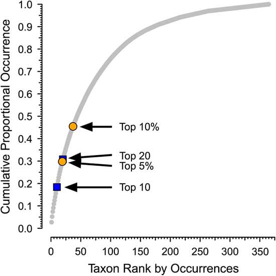
Second, although there is qualitative recognition of when a taxon is common and when it is rare, there is no ecological or paleontological consensus on the criteria on for this or even a generally used term to refer to common taxa. For example, although Hannisdal et al. (Reference Hannisdal, Haaga, Reitan, Diego and Liow2017) characterize taxa with high site occupancy on a global level as being common, they do not propose a cutoff between common and not common. There is no obvious natural separation between common and less common taxa in the PaleoDB. Although the distribution of number of occurrences per taxon is heavily skewed, as shown in Plotnick and Wagner (Reference Plotnick and Wagner2006), it is continuous and without natural breaks. For example, the cumulative proportion of occurrences versus rank for brachiopods in the Permian 3 bin is shown in Figure 1 (see also Supplementary Fig. 1).

Figure 1 Sample distribution for occurrences of brachiopod genera in the Permian 3 bin of the Paleobiology Database, showing cumulative proportion of occurrences vs. rank. There are 311 brachiopod genera, with a total of 13,316 occurrences. The arrows indicate different potential cutoffs between dominant (“common”) and nondominant genera (see Table 1). Permian 3 corresponds to the Roadian to Capitanian stages (Guadalupian series). Paleobiology Database data downloaded 22 January 2018.
In this paper, we will use “dominant” to refer to genera that are responsible for a disproportionate share of occurrences within defined higher taxa in a particular time bin. We distinguish dominant from nondominant taxa based on ranking of the genera by the number of occurrences in a temporal bin, with dominant genera ranking as either the top 10 within a target class or top 20 for all six target classes combined. Although these divisions are arbitrary, they are a consistent way to make the separation (Fig. 1, Table 1, Supplementary Fig. 1). In addition, because only a relatively small fraction of all genera would be considered dominant under any criterion (Table 1; Plotnick and Wagner Reference Plotnick and Wagner2006), this division should capture the overall picture. Nevertheless, we also provide results using “top 5%” (for all taxa) and “top 10%” (for individual clades) as a criterion in two analyses as a sensitivity analysis.
Table 1 Effect of different cutoffs between dominant (“common”) and nondominant taxa in the Paleobiology Database. Data are number of occurrences per genus for brachiopods in the Ordovician 5 (Late Ordovician) and Permian 3 (Guadalupian) bins and bivalves in the Cenozoic 5 (Miocene: Aquitanian–Serravallian) bin. Cutoffs are: 10 most common genera (top 10); 20 most common genera (top 20); and top 5%, 10%, and 20% of all genera. Values are the cumulative percentages of all occurrences at those cutoffs (see Fig. 1). Paleobiology Database data downloaded on 22 January 2018.
A third, and potentially the most contentious issue, is the nature of an occurrence in the PaleoDB, where “occurrence” is the recorded presence of a member of a species or genus at a fossiliferous locality or site (Buzas et al. Reference Buzas, Koch, Culver and Sohl1982). Localities in the PaleoDB vary widely in their properties; some are closely sampled, temporally restricted, ecologically defined, and spatially discrete, whereas others can be very general in their stratigraphy, environment, and spatial location. Our approach does not assume that fossiliferous localities in the database are all equivalent as units of sampling or as macroecological entities. Instead, it assumes that there are no secular trends in the nature of the sites recorded. Thus, although PaleoDB occurrences almost certainly vary as units of space and ecology, there is no need to think that this might create any patterns or even that the range of variation greatly exceeds that of many modern ecological studies. This assumption should be tested as part of a future assessment of data quality in the PaleoDB.
Occurrences and Occupancy
An important related issue is the relationship of PaleoDB occurrences to the ecological concept of occupancy and its usage in paleontology. Bailey et al. (Reference Bailey, MacKenzie and Nichols2014) defined occupancy as “the probability that the focal taxon occupies, or uses, a sample unit during a specified period of time during which the occupancy state is assumed to be static” (p. 1270). Both in ecology and paleontology, there is no set diagnosis for the sampling unit that can be repeated from one study to the next. As pointed out by Steenweg et al. (Reference Steenweg, Hebblewhite, Whittington, Lukacs and McKelvey2018), the operational definition of occupancy, the proportion of sampling units where a species is found, is dependent on how the units are spatially and temporally delineated. In terms of space, patch occupancy refers to occupation of a discontinuous habitat patch, such as finding a particular species of fish within a set of ponds. Alternatively, a region can be divided up by an equal-area grid into cells. In this case, cell occupancy measures the number of cells that are occupied by the species of interest. Finally, site occupancy looks at presence or absence of the species at or near a set of discrete sampling points, such as traps, which may or may not be evenly distributed.
Cell occupancy is not applicable to most fossil groups. As shown by Plotnick (Reference Plotnick2017), the distribution of fossil localities is disjunct and patchy at many scales, resulting from multiscaled controls on their formation, preservation, and discovery. Many of these processes are geological and anthropogenic, rather than biological. As a result, it is difficult or impossible to define a consistent criterion for a region of interest or how it should be subdivided into sampling units. For this reason, we have not used such a spatially explicit sampling scheme here, although we have used a correction for local heterogeneity in sampling intensity.
Paleontological studies of occupancy have used concepts closer to patch or site occupancy, or some combination. Foote et al. (Reference Foote, Crampton, Beu, Marshall, Cooper, Maxwell and Matcham2007) suggested that the relationships among local abundance, geographic range, and proportion of the range that is occupied jointly be termed “occupancy,” with an operational measure as the proportion of collections in which a species occurs. Foote (Reference Foote2016) widened his description of the set of sampling entities to include “sites, collections, geographic areas, or other sampling units.”
Liow (Reference Liow2013), in her application of occupancy models to paleontological data, defined occupancy as the “probability that a randomly selected sampling unit within a defined region is occupied by the taxon of interest regardless of whether this taxon is sampled in that particular sampling unit” (p. 194). The use of probability, in the context of the modeling, was to include the possibility that a taxon was not sampled, rather than not present (see also MacKenzie et al. Reference MacKenzie, Nichols, Lachman, Droege, Andrew Royle and Langtimm2002, Reference MacKenzie, Nichols, Hines, Knutson and Franklin2003, Reference MacKenzie, Bailey and Nichols2004; Bailey et al. Reference Bailey, MacKenzie and Nichols2014). Liow illustrated the approach using the Cincinnatian brachiopod, Hebertella. In this example, the sampling unit was identified as being equivalent to a PaleoDB collection, being from a single bed at a specific locality. This is generally equivalent to site occupancy. In contrast, her more complex model defined sites as being defined not only by geographic location, but by stratigraphic position in a depositional sequence and by facies. Multiple collections from the same combination were considered replicate samples within sites. This approach to occupancy thus more closely resembles patch occupancy.
Hannisdal et al. (Reference Hannisdal, Haaga, Reitan, Diego and Liow2017) used temporally binned planktonic foraminiferal occurrences in the Neptune Database, which is based on ocean-drilling locations. These are clearly site occupancy, with high-occupancy species occupying a higher proportion of sites within a bin. These proportions were summed to calculate their summed common species occurrence rate (SCOR) metric, whose value is highly dependent on the most common species in the bin. This is useful for contrasting occupancy or occurrence structure among different intervals or taxa. However, our goal is to compare patterns among common taxa in different data subsets as well as between common and noncommon taxa.
In this study, our sampling units are defined by taxonomy and temporal bin; that is, we are including all database localities that have at least one genus-level occurrence of the classes or classes of interest and are within one of the PaleoDB roughly 10 Myr bins (Alroy et al. Reference Alroy, Aberhan, Bottjer, Foote, Fürsich, Harries, Hendy, Holland, Ivany, Kiessling, Kosnik, Marshall, McGowan, Miller, Olszewski, Patzkowsky, Peters, Villier, Wagner, Bonuso, Borkow, Brenneis, Clapham, Fall, Ferguson, Hanson, Krug, Layou, Leckey, Nürnberg, Powers, Sessa, Simpson, Tomasovych and Visaggi2008). We do not include localities that do not contain a representative of a target group. Unlike explicit occupancy studies, however, our denominators are not the number of localities. Instead, they are the summed count of all occurrences of all genera of a target group within a bin; they are thus a product of both the number of sites that contain that class and the total diversity. For example, if two genera coexist at the same locality, then each has half of the occurrences; but if one is found at one locality and the other at another, then each still has half the occurrences. For this reason, although 3.62% of all occurrences of brachiopods in the Permian 3 bin are assigned to Hustedia, whereas 1.63% belong to Meekella, this does not directly imply that the former is found in twice as many localities as the latter.
Plotnick and Wagner (Reference Plotnick and Wagner2006) combine all Phanerozoic occurrences within their target taxa and do not examine temporal changes among the common taxa. The goal of the current paper is to examine the tendencies of the most dominant taxa over very long intervals of time and to compare these patterns to those of less common taxa. Specifically, akin to Reddin et al. (Reference Reddin, Bothwell and Lennon2015), we seek to answer whether dominant taxa are fundamentally different from nondominant taxa. We do this in three ways. First, we look at changes in dominant genera from bin to bin by ranking them and then examining turnover within the top ranks. For example, what proportion of the 20 most common brachiopod genera from one interval of the Ordovician also appear in that list in the next interval of the Ordovician? If general extinction dynamics affect these dominant genera as they do all genera, then we expect to see common patterns of turnover. Alternatively, if dominant genera have properties that make them less prone to extinction than the majority of genera, then their turnover patterns should be different. This analysis is done for six target groups of major Phanerozoic taxa separately and combined to determine whether persistence of individual genus dominance differs among the different higher taxa. If the general differences in evolutionary dynamics among higher taxa affect their dominant genera, then persistence of dominant taxa within them should reflect previously documented differences in their evolutionary dynamics.
Second, we compare bin-to-bin origination and extinction rates of dominant and nondominant genera. If common taxa are more persistent over time than nondominant taxa, these rates should be lower than for more transient nondominant genera.
Third, we study the patterns of rise and fall of dominant taxa and determine whether they are measurably different from the histories of nondominant genera (Foote Reference Foote2007). If dominant genera possess characteristics that give them an immediate advantage, then they may rise in dominance more rapidly than would be the case among a more typical taxon. Alternatively, they might also have properties that allow them to persist at high levels of commonness longer than the majority of genera. This would again be the situation if they are more resistant to extinction.
Finally, we also briefly reconsider explanations for the existence of dominant taxa. Plotnick and Wagner (Reference Plotnick and Wagner2006) examine possible reasons for a taxon to be dominant in terms of the number of occurrences. This could represent biological signal, such as is the case with modern common species. Alternatively, they could represent artifacts of taxonomic practice. Here, we present a simple model of morphological and phylogenetic diversification and sampling that might account for some dominant taxa.
Data
We analyze brachiopods, gastropods, bivalves, cephalopods, trilobites, and echinoids. The basic data are the occurrences (appearance of a genus name in a collection) for each genus of these groups downloaded from the PaleoDB in October 2013, grouped into one of 49 bins approximately 10 Myr each in duration (Alroy et al. Reference Alroy, Marshall, Bambach, Bezusko, Foote, Fürsich, Hansen, Holland, Ivany, Jablonski, Jacobs, Jones, Kosnik, Lidgard, Low, Miller, Novack–Gottshall, Olszewski, Patzkowsky, Raup, Roy, John Sepkoski, Sommers, Wagner and Webber2001, Reference Alroy, Aberhan, Bottjer, Foote, Fürsich, Harries, Hendy, Holland, Ivany, Kiessling, Kosnik, Marshall, McGowan, Miller, Olszewski, Patzkowsky, Peters, Villier, Wagner, Bonuso, Borkow, Brenneis, Clapham, Fall, Ferguson, Hanson, Krug, Layou, Leckey, Nürnberg, Powers, Sessa, Simpson, Tomasovych and Visaggi2008). The data that we use come from 6315 studies and/or published data sets. Twenty studies contributed more than 1400 records each (King Reference King1931; Reed Reference Reed1944; Gardner Reference Gardner1947; Besairie and Collignon Reference Besairie and Collignon1972; Cooper and Grant Reference Cooper and Grant1977; Toulmin Reference Toulmin1977; Woodring Reference Woodring1982; Sohl and Koch Reference Sohl and Koch1983, 1984, Reference Sohl and Koch1987; Gitton et al. Reference Gitton, Lozouet and Maestrati1986; Manivit et al. Reference Manivit, Le Nindre and Vaslet1990; Aberhan Reference Aberhan1992; Tozer Reference Tozer1994; Jablonski and Raup Reference Jablonski and Raup1995; Stygall-Rode and Lieberman Reference Stygall-Rode and Lieberman2004; Holland and Patzkowsky Reference Holland and Patzkowsky2007. A full bibliography is given as in the Supplementary Material (see also Wagner et al. Reference Wagner, Plotnick and Lyons2018).
We exclude genus-only records (e.g., Bellerophon sp. or Turritella sp.) for two reasons. One, the relational taxonomic fields in the PaleoDB cannot “correct” the generic occurrence if the unnamed sampled species subsequently is reassigned to another genus. Two, many such occurrences fall outside the stratigraphic ranges of named species placed in those genera, which casts doubt on the veracity of the assignments (Wagner et al. Reference Wagner, Aberhan, Hendy and Kiessling2007). For the remaining records, we vet species’ names extensively. This includes checking for misspelling and converting all specific names to gender-neutral versions so that “umbilicata,” “umbilicatus,” and “umbilicatum” all are considered to be the same species name (Wagner et al. Reference Wagner, Plotnick and Lyons2018).
We treat subgenera as genera. In part, this simply follows the protocols of earlier diversity studies using genera (e.g., Sepkoski Reference Sepkoski1997). However, this also is because genera and subgenera are used inconsistently in published papers and thus in the data entered in the PaleoDB. Although taxonomic fields “fix” these ranks to the latest opinion in many genera/subgenera, they do not yet do so for all cases.
Many collections represent different beds from the same formation in the same densely sampled stratigraphic section. A genus might be known only from that formation at that section yet have many occurrences by being found in multiple beds within a few meters of each other. Similarly, there are some general areas in which sediments from a general time interval are very well sampled (e.g., Middle and Upper Ordovician strata from the Cincinnati Arch region.) Moreover, the highly uneven spatial patterns of sedimentary rocks make the distributions of localities clumped (Plotnick Reference Plotnick2017). Such “binge sampling” will raise commonness estimates for taxa restricted to those regions (see Raup Reference Raup1972). This also introduces another major way in which fossil occurrences differ from occupancy: in principle, a taxon occupying one area might have many occurrences if that area is well sampled. We control for this by only counting localities from the same formation that were greater than 1 km away from the closest locality from that formation also bearing the species in question. (In cases in which rock units are ranked as members in some papers but formations in others, we used the latest opinions of that unit [Darroch and Wagner Reference Darroch and Wagner2015; Wagner et al. Reference Wagner, Plotnick and Lyons2018].) Thus, if there are three localities from Formation X within 1 km of each other, one “unique” locality is tallied for species occurring at those three localities. The result is that each locality effectively equals a 2-km-diameter equal-area bin.
After “correcting” for binge sampling, we analyze those species (and genera) representing 248,938 occurrences from 28,259 localities. Counting each combination of taxon and time independently (i.e., each genus that occurs in multiple bins is tallied for each bin), there were a total of 31,058 total combinations of genus and time bin.
Methods
For each of the six focal classes, we rank each genus in each bin by number of occurrences. This includes both extinct and extant genera. We also rank genera within a pooled group of the classes. For our first analysis, we consider a genus to be dominant if it ranked within the top 10 or the top 20 within its class. Because some classes had very low generic richness in some bins (e.g., echinoids in Jurassic 3), we only use bins with at least 40 genera in both that bin and the prior one. The top 10 typically captured between 15% and 20% of all occurrences for their class in a bin. For analyses using all six classes, genera in the top 20 (including those tied for number 20) are considered dominant.
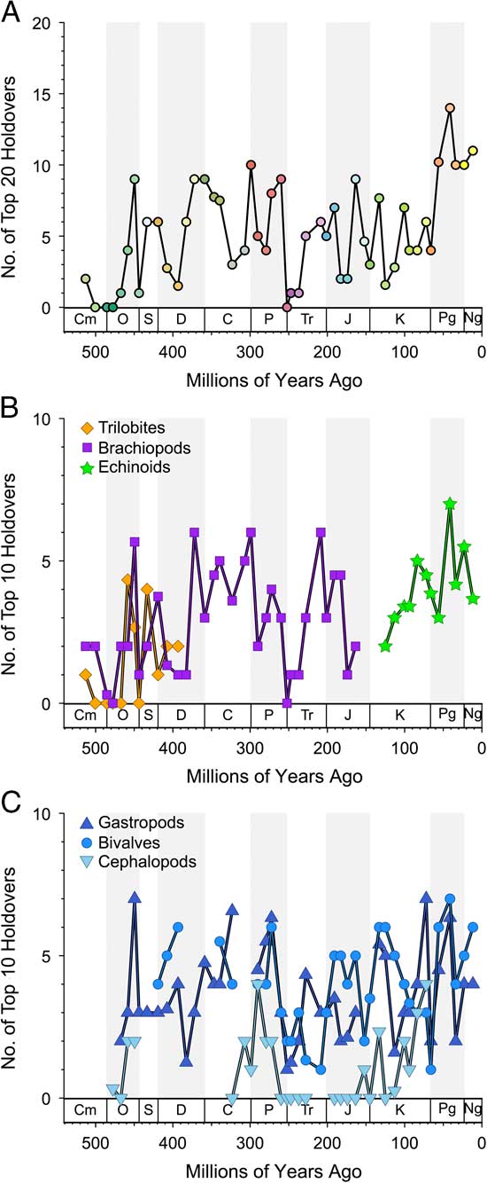
As a measure of turnover among dominant genera, we determine how many dominant genera in a bin are holdovers from that status in the previous bin, independent of exact rank in that group (Fig. 2A, Table 2). For the combined classes, in cases in which there are two or more genera sharing the rank of number 20, we add the proportion of number 20 genera that are holdovers to the number of the top 19 that are. So, if 9 of the top 19 are holdovers, and 3 of 5 genera tied at number 20 are holdovers, then we tally 9+⅗=9.6. To determine whether the different classes show matching patterns of turnover, we use Spearman’s rank correlation test to measure associations among unlagged time series for the different classes (Table 3). We also performed an analysis in which we examined turnover among the top 5% of all genera per bin for the combined classes and the top 10% of all genera per bin for individual clades (Supplementary Fig. 2). Holdovers here are shared genera divided by the maximum possible shared genera: if one interval has 20 genera in the top 5% and the next has 22 genera, then they can share (at most) 20 genera.

Figure 2 Holdovers within “top 20” or “top 10” over time. Values are numbers of most common genera on that list from one bin that are found in the next. Zero is complete turnover on the list (Supplementary Tables 1, 2). A, Top 20 (top 21 in case of ties) for all taxa merged. B, Top 10 for trilobites, brachiopods, cephalopods, and echinoids. C, Top 10 for gastropods, bivalves, and cephalopods. Only intervals with more than 50 genera are shown.
Table 2 Minimum, maximum median, and average of top 10 and top 20 holdovers over time within each of the six target groups. Gastropods, echinoids, and bivalves show high numbers of holdovers from prior list of high ranks relative to other taxa.

Table 3 Cross-correlations at zero lag among the top 10 holdover series (Fig. 2) for the six target classes. Data in Supplementary Table 1. Lower left: Spearman’s rank correlation coefficient using pairwise deletion, with number of pairs given in parentheses. Upper right: Pearson’s product moment correlations, with p-values given in parentheses. Values below standard 5% cutoff are in bold and are not corrected for multiple comparisons or autocorrelation. “x” indicates no overlap.

In our second analysis, we consider a dominant genus to be one that either reaches the top 20 or was among the top 5% for at least one bin within the combined six target classes. We calculate absolute rates of origination and extinction among only those genera and among only the remaining genera. These rates are comparable to similar rates calculated by other studies using the entire pool of genera (Alroy et al. Reference Alroy, Aberhan, Bottjer, Foote, Fürsich, Harries, Hendy, Holland, Ivany, Kiessling, Kosnik, Marshall, McGowan, Miller, Olszewski, Patzkowsky, Peters, Villier, Wagner, Bonuso, Borkow, Brenneis, Clapham, Fall, Ferguson, Hanson, Krug, Layou, Leckey, Nürnberg, Powers, Sessa, Simpson, Tomasovych and Visaggi2008).
Similarly, in the third analysis, we again focus on the individual classes and consider a dominant genus to be any within the class that were in the top 10 for at least one bin. We consider only extinct genera that ranged over at least three bins. Using only extinct genera restricted the study to taxa with (apparently) completed histories; note that this eliminates many high-ranked extant Cenozoic taxa, such as Turritella. For every genus, we count how many times it was on the top 10 list (count) and the sum of its ranks within that list for those bins (summed ranks), where 10=rank number 1 (most common) in the bin to 1 for rank number 10 (10th most common). Taxa with tied rankings are given the average ranking (e.g., 2.5 for two tied for second), allowing for noninteger ranks. For example, a genus that remains in the top 10 for three bins and has ranks of 7, 2, and 4 within those bins would have a count of 3 and a summed rank of 20, whereas a genus that was ninth most dominant for a single bin would have a count of 1 and a summed rank of 2. High values of summed ranks and counts for a genus thus indicate greater dominance for longer periods of time. We produce frequency distributions of number of counts and of summed ranks for each taxonomic class. Because classes were of different total sizes, we divided total counts and the total summed ranks for each group by number of genera within the bins (Table 4). Higher mean values for both metrics represent greater persistence at higher rank for the genera in the class, for example, lower turnover at the top ranks.
Table 4 Counts and summed ranks for each class. Counts are the total number of times a genus ranks in the top 10 in a bin; summed ranks are the sum per genus of 10=rank number 1 in the bin to 1 for rank number 10 in the bin over all bins in which the genus occurs. Higher mean values for both metrics represent greater persistence at higher rank for the genera in the class (e.g., lower turnover at the top ranks). Taxa with tied rankings are given the average ranking (e.g., 2.5 for two tied for second), allowing for noninteger ranks.
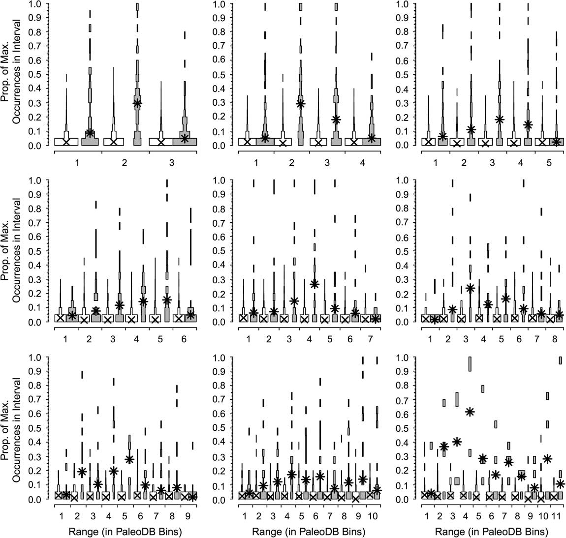
In the next two analyses, we again use the combined six target classes and define a dominant genus as one that reaches the top 20 for at least one bin. We divide the number of occurrences for each genus by that of the most dominant genus in that interval to calculate the proportion of maximum occurrences per interval; for example, a value of 0.2 means a genus has 20% of the occurrences of the most common one in that bin. Unsampled range-through genera are included, with a score of 0%. We rescale occurrences relative to the most commonly occurring genus for two reasons. One, we expect the most common genus in an interval with 1000 collections to have about twice the occurrences of the most common genus in an interval with 500 collections. Two, we expect the most common genus in a bin with high beta diversity to have fewer occurrences than the most common genus in a bin with low beta diversity. Thus, this “relative dominance” offers a partial correction for both sampling and biological factors affecting how many occurrences we expect from comparably dominant genera in different time bins. We did this for taxa with durations of 3 to 11 bins (Fig. 3). Thus, for all genera that persisted for three bins (regardless of whether those three bins were in the Ordovician or the Cenozoic), we determined the relative dominance in bins 1, 2, and 3 for both the dominant (Fig. 4, gray boxes) and rarer genera (Fig. 4, white boxes). If a genus is very common relative to the most common contemporaneous genus when it first appears, then it will have a high value in the first bin; conversely, a high value in the last bin implies the genus was very common relative to the most common genus when it was last sampled. We calculate the medians of the frequency distributions for the top 20 (Fig. 4, asterisks) and the remaining genera (Fig. 4, crosses). This analysis allows us to assess whether there is a difference in the trajectories of relative dominance between dominant and rarer genera and whether there are differences between short-ranged and long-ranged genera. We also compared the ranks of common and less common genera at the times of first and last appearance (Fig. 5).
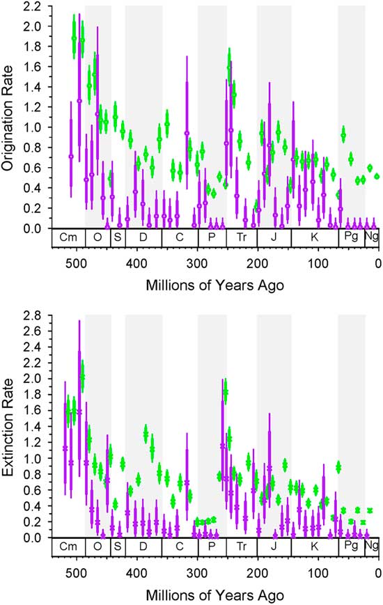
Figure 3 Bin-to-bin origination and extinction rates for dominant (purple) and nondominant (green) genera from the intervals noted. Dominant are always first, so compare left to right. These values take into account sampling in the prior interval based on the distribution of samples in the prior interval. The thick bars are 1-unit support, and the thin bars are 2-unit support. If the thick lines do not overlap, then the difference is significant. The column on the left is for using top 20 as a criterion for dominance; the column on the left is for top 5% as the criterion.

Figure 4 Dominance patterns over time for the genera that rank in the top 20 in a Paleobiology Database bin at some point (gray spindles) compared with all other genera (white spindles). Results are shown for all extinct genera that last for between 3 and 11 bins. Ordinate is the distribution of the proportion of maximum occurrences in the interval, a measure of relative importance (see text). The values for the common genera show little change over time; those of the dominant genera show a pattern of waxing and waning, but rarely are common at first or last appearance.

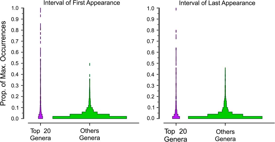
Figure 5 Relative importance of top 20 and other genera in their first and last intervals, based on proportion of maximum occurrences (see text). The first Cambrian interval from the first appearances and the last Cenozoic interval from the last appearances are omitted.
In our final analysis, we use center-of-gravity (CG) statistics to examine the patterns of rise and fall of the dominant and rarer taxa in the combined six classes. CG statistics are often used to assess the symmetry of historical patterns of richness (e.g., Gould et al. Reference Gould, Gilinsky and German1987; Uhen Reference Uhen1996) and morphological disparity (e.g., Foote Reference Foote1992; Hughes et al. Reference Hughes, Gerber and Wills2013). A CG of 0.5 indicates a perfectly symmetric rise and fall, with peak relative occupancy tending to be in the middle of a genus’s sample history; CG values >0.5 indicate a more rapid rise than fall (bottom-heavy), whereas CG values >0.5 show a slower rise than fall (top-heavy). Here, we ask whether symmetry in occupancy over time (again, scaled relative to the most commonly occurring genus in a bin) differs among dominant and nondominant genera (Fig. 6).
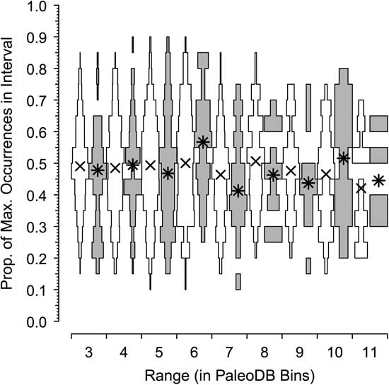
Figure 6 Centers of gravity (CGs) for extinct dominant genera (gray) and the remainder (white) having ranges of 3 to 11 Paleobiology Database bins, based on proportion of maximum occurences (see text). Asterisks (*) are median values for dominant genera; crosses (×) are median values for the remainder. For both dominant and nondominant genera, the CGs are in the middle of the range (CG≈0.5).
Results
The turnover history among common (“top 20”) genera within the six combined classes over time is shown in Figure 2A (data in Supplementary Table 2). What stands out in this plot is that even though these common genera represent less than 5% of all genera and the holdover metric considers only ~20 genera in any bin, the overall pattern still resembles those seen in many plots of total biodiversity fluctuations (e.g., Raup and Sepkoski Reference Raup and Sepkoski1982; Alroy et al. Reference Alroy, Aberhan, Bottjer, Foote, Fürsich, Harries, Hendy, Holland, Ivany, Kiessling, Kosnik, Marshall, McGowan, Miller, Olszewski, Patzkowsky, Peters, Villier, Wagner, Bonuso, Borkow, Brenneis, Clapham, Fall, Ferguson, Hanson, Krug, Layou, Leckey, Nürnberg, Powers, Sessa, Simpson, Tomasovych and Visaggi2008; Zaffos et al. Reference Zaffos, Finnegan and Peters2017). Notable examples include a ramp-up in holdovers during the great Ordovician biodiversification event (GOBE); sharp drops at the ends of the Ordovician, Permian, and Cretaceous; and a rise to a stability maximum during the Cenozoic.
When we consider holdovers in the top 5% rather than the top 20, there are slight differences in the overall pattern (Supplementary Fig. 2), but they are highly correlated (Supplementary Fig. 3). In general, we tend to see higher holdover proportions when using the top 5% instead of the top 20. The median number of genera in the top 5% is 27, which suggests that many top 20 taxa are lurking just under the top 20 in the prior or subsequent intervals.
The turnover patterns for the six target classes are shown individually in Figure 2B and C (data in Supplementary Table 1). In these plots we are considering only the top 10 genera within each bin. Not surprisingly, the patterns resemble the overall patterns for bins in which the class itself is dominant; for example, changes in dominance in brachiopods are reflected in the Paleozoic top 20. What is striking here is that the average and maximum number of holdovers among common genera is higher for the echinoids, gastropods, and bivalves than for brachiopods, and much higher than for cephalopods and trilobites (Table 2). Pairwise Mann-Whitney tests comparing the median of top 10 and top 20 holdovers among the classes are significant at p<0.001, with the exception of bivalves and gastropods, which are not significant (p=0.97 for top 10; p=0.89 for top 20). Despite the strong similarities at key points such as the mass extinction intervals and the GOBE, none of the sequences are highly cross-correlated using Spearman’s rank correlation test (Table 3). Of the 15 pairwise comparisons, five are significant at p<0.05 for Pearson cross-correlations, with the lowest p-value for the comparison between cephalopods and bivalves. Echinoids are negatively correlated with all other groups (except trilobites, with which they do not overlap). The correlations were not corrected for multiple comparisons or autocorrelation.
The histories of originations and extinctions within common and less common taxa are illustrated in Figure 3; in this case we use a less restrictive definition of “common,” in that a common taxon has only to reach the top 20 ranks or top 5% for a single bin. As would be expected, both origination and extinction rates for the common genera (Fig. 3, purple) are much lower than those for the nondominant taxa (Fig. 3, green); for example, many of the nondominant taxa are singletons. Common taxa genera are less affected by the end-Devonian and end-Cretaceous mass extinctions than are less common taxa. However, common and less common genera show indistinguishable extinction rates for the end-Ordovician, end-Permian, and end-Triassic. Again, there are only trivial differences in the results based on choice of cutoff, indicating that our results are robust to changes in this parameter.
Comparisons of counts and summed ranks among the six target classes are summarized in Table 4. The classes are sorted by mean values for both metrics, with higher values indicating greater persistence of genera at top ranks. The most commonly occurring genera typically last many more intervals at the top in bivalves than in trilobites or cephalopods, with gastropods and echinoids close behind bivalves, and brachiopods intermediate. Within these two basic partitions, dominant bivalves might show significantly greater persistence than dominant gastropod genera, and dominant brachiopod genera clearly show significantly greater persistence than dominant cephalopod or trilobite genera.
Contrasts in the dominance trajectories between common and nondominant genera as a function of their duration are shown in Figure 4. For the majority of the genera (Fig. 4, white boxes), there are no noticeable shifts in their relative dominance during their ranges; they remain relatively rare throughout. In contrast, dominant genera (Fig. 4, gray boxes) are in most cases already slightly more important at the time of their first appearance and increase their dominance in the middle of their range, and then fall back but remain relatively important at the time of their extinction (Fig. 5). It is relatively rare, however, for a common genus to be at the top at the very beginning or the very end of its range or to be common throughout its range. Peaks can occur throughout the range of a genus. The pattern is less clear for the longest-lived taxa, but there are very low numbers of these forms, and they are more apt to be affected by mass extinctions toward the ends of their ranges. The two groups differ significantly from each other in both cases: although common genera rarely are “common” at the outset, they also are much less apt to start off very rare than are nondominant genera. Common genera are also more likely to be fairly common at their last appearance.
The horizontal axes of Figure 6 plot the distribution and median CGs, with 95% error bars added, for taxa that persist for 3 to 11 bins. What stands out is that the centers of gravity are not different. Similar to the results of Foote (Reference Foote2007), the CG tends to be in the middle of the range for both common and nondominant genera, indicating a pattern of symmetrical rise and fall.
Discussion
The key issue we examine is whether the dominant genera are fundamentally different in some way from nondominant genera or if they are simply genera that just happen to have a greater share of total occurrences. We find some support for both alternatives. First, overall turnover patterns within dominant genera, which represent only a small fraction of total richness, still resemble those seen based on estimates of total biodiversity fluctuations (Harnik et al. Reference Harnik, Lotze, Anderson, Finkel, Finnegan, Lindberg, Liow, Lockwood, McClain, McGuire, O’Dea, Pandolfi, Simpson and Tittensor2012). For example, episodes of major drops in the dominant positions of these taxa mirror the decline of overall richness associated with mass extinction intervals. Thus, the mechanisms of the major mass extinctions are capable of eliminating or at least greatly reducing widespread and often locally abundant genera, and presumably their constituent species. As suggested by Hull et al. (Reference Hull, Darroch and Erwin2015), rarity of previously abundant species is essentially equivalent to extinction, because it requires the extirpation of multiple populations. Previous studies of patterns of ecological change in the fossil record, especially of extinctions, have recognized that there is a decoupling between biodiversity changes and ecosystem alterations (Droser et al. Reference Droser, Bottjer and Sheehan1997, Reference Droser, Bottjer, Sheehan and McGhee2000; Christie et al. Reference Christie, Holland and Bush2013; McGhee et al. Reference McGhee, Clapham, Sheehan, Bottjer and Droser2013). Thus, either the extinction of a dominant taxon has a much greater ecological impact than that of nondominant ones, or far greater ecological perturbations are needed to eliminate dominant genera. Discussions of extinction mechanisms therefore need to consider how these dominant taxa can disappear (e.g., Jablonski Reference Jablonski2005).
Second, comparisons of turnovers among classes within dominant genera generally reflect previously established differences in evolutionary dynamics among these classes. In this regard, dominant genera among classes have less in common with one another than they do with the nondominant members of their own class. Thus, the fact that bivalve genera such as Inoceramus and gastropods such as Turritella persist as high-occupancy genera, whereas dominant trilobite and cephalopod genera never remain dominant for long, probably reflects differences among gastropods and bivalves relative to cephalopods and trilobites rather than anything unique to those bivalve and gastropod genera (see Stanley Reference Stanley1990; Valentine Reference Valentine1990; Connolly and Miller Reference Connolly and Miller2001). Nevertheless, another factor that merits exploration is whether genera such as Inoceramus or Turritella might be unusually conservative morphologically for bivalves and gastropods. If so, then the “inability” of such genera to frequently give rise to species sufficiently distinct as to merit a new genus name might elevate their species richnesses and total occupancy even more than expected, given the relatively low turnover rates of bivalves and gastropods. This might also prove to be true for trilobites and cephalopods with higher turnover, but the greater sample sizes and longer periods of time will make this idea easier to test with the bivalves and gastropods.
Third, rates of both origination and extinction in dominant taxa tend to be lower than those of nondominant taxa. This suggests that dominant genera will be longer lived than nondominant ones.
Finally, the shapes of the trajectories of the two groups are similar, with a symmetrical rise and fall. Dominant genera are somewhat more likely than nondominant taxa to be relatively common when they first appear in the record, although they are rarely dominant in their first interval. Dominant genera generally do not reach that status immediately, but instead first appear relatively common and then rise to dominance. Genus-level occupancy correlates with species richness (Supplementary Fig. 4), which could reflect dominant genera commonly debuting with a small number of common species. Dominant genera also tend to decline from dominance before their last appearance, although they still tend to be relatively common at their last appearance.
In sum, there is some validity to the concept of a dominant taxon, although such taxa are end members of a continuum, rather than a discrete class (Fig. 1, Supplementary Fig. 1). This raises the issue of why a genus would be dominant. Plotnick and Wagner (Reference Plotnick and Wagner2006) suggest a number of possibilities. Dominance might represent an actual biological signal, wherein the genera are truly widespread and abundant with a long stratigraphic range. A second option is that they have a higher than average preservation potential. There is also the possibility that we are capturing biases within the PaleoDB rather than a true signal; in particular, much of what we see may not be global, but reflects the preponderance of localities in North America and Europe. Another option is that, as discussed in detail in Plotnick and Wagner (Reference Plotnick and Wagner2006), many dominant genera might also be taxonomic wastebaskets. Those authors found that, on average, dominant genera were first described in the nineteenth century (this is also true of widespread extant mammal species; Plotnick et al. Reference Plotnick, Smith and Lyons2016) and thus might be the default taxonomic assignments for subsequent described collections.
Related to this last possibility is that dominant genera are nearly three times more apt to be the type genus of a family or subfamily than are rarer genera: 320 of the 718 dominant genera are types given current (2016) classification in the PaleoDB, whereas 2020 of 12,361 rarer genera are types for their families or subfamilies. The genus typifying a family might become the default generic assignment for species in that family, artificially elevating how common it is (Wagner et al. Reference Wagner, Aberhan, Hendy and Kiessling2007; Hendricks et al. Reference Hendricks, Saupe, Myers, Hermsen and Allmon2014).
Here we suggest two other options that reflect the interaction of biological patterns with taxonomic practice. First, occurrences among genera correlate strongly with species richness within genera (Liow Reference Liow2007; Foote et al. Reference Foote, Ritterbush and Miller2016; Supplementary Fig. 3). Thus, we expect morphotypes with many species to be easier to sample than those with few species. Over the history of paleontology as a science, we expect species from speciose genera to be described in earlier works than species from species-poor genera. That in turn also elevates the chance that such genera will wind up as types for families.
Another explanation is that dominant genera reflect the pattern expected, given a simple model of character evolution, diversification, and taxonomic practice that predicts greater species richness among “primitive” genera than derived ones (e.g., Raup and Gould Reference Raup and Gould1974; Estabrook Reference Estabrook1977; Uhen Reference Uhen1996; Wagner and Estabrook Reference Wagner and Estabrook2014). Consider a genus that originates with a single species with character states 0000 that are used to diagnose and define the genus. Because of phylogenetic autocorrelation, most daughter species also will share these character states. However, at some point, a daughter species with character states 1000 will appear and will be placed in a new genus (Patzkowsky Reference Patzkowsky1995). At the time the new genus evolves: (1) there usually will have been multiple earlier species with the original 0000 combination; and (2) there usually will be several coexisting species with combination 0000 compared with only one with 1000. Unless a species with character states 1000 actively supplants those with 0000, subsequent descendants of the original species probably will evolve from a 0000 species rather than from the 1000 species (or its possible descendants). Thus, new clade members will more probably inherit the traits of the paraphyletic genus (0000) than the derived one (1000). The result is that the paraphyletic genus defined by 0000 usually will be more speciose, and thus probably will have more occurrences that the monophyletic genus defined by 1000. The combination of being speciose and common and having a more common general morphology would make it more likely that systematists would deem 0000 appropriate for typifying a subfamily or family. Indeed, it also makes it more probable that paleontologists will have sampled species with 0000 before they have sampled those with 1000. Of course, exactly why individual “dominant” genera succeeded, and the extent to which this represents macroecological success independent of macroevolutionary success, requires more detailed analyses than we can offer here, but our results are entirely consistent with the expectations that broad distributions and diversification often go hand in hand (e.g., Brown Reference Brown1984).
A corollary of our argument is that the general congruence of the patterns seen in the dominant genera with those in the much larger compilations of described fossil genera should not be surprising. As discussed earlier, dominant genera, because they are both common and widespread, are highly likely to be among the earliest to be taxonomically described. Their appearance and disappearances have thus been familiar since the earliest compilations of biodiversity history (Sepkoski et al. Reference Sepkoski, Bambach, Raup and Valentine1981) and certainly long predate the iconic Sepkoski compendium of genera (Sepkoski Reference Sepkoski2002). In effect, we have “rolled back” decades of taxonomic work to show, as Sepkoski et al. (Reference Sepkoski, Bambach, Raup and Valentine1981) suggested, that the basic patterns are robust.
One possibility worth examining in the future is that dominant genera typically were descended from other dominant genera, and thus that part of their early relative success is inherited from successful ancestors. There is limited evidence that occurrence rates and occupancy rates show phylogenetic autocorrelation among species within relatively small clades (e.g., Wagner Reference Wagner2000; Carotenuto et al. Reference Carotenuto, Barbera and Raia2010). Our data here are consistent for this within genera: genera probably are apt to have fewer species in their first interval than in later intervals, which means that the relatively high occupancy of dominant genera early in their histories is accomplished with few species.
There is almost certainly no single reason why a taxon is common, either locally or globally. A detailed case-by-case study will need to be made at some point to investigate this issue; but that is beyond the scope of this paper.
Finally, we want to raise the issue of whether the patterns we have shown for dominant genera mirror more general patterns for success in other systems, including anthropogenic ones. In this we are influenced by West (Reference West2017), who argues that the processes that govern survival of organisms, cities, and corporations may have universal mathematical properties. One property of corporate success he discusses is being listed on the Standard & Poor’s 500 Index or Fortune magazine’s list of 500 most successful companies. West points out that most companies have a finite lifetime on these lists; currently the average survival in about 18 years. We looked at the list of top 500 global companies published by the Financial Times; of the top 10 companies in 2002, only four were ranked that high in 2013. Other fields in which relative success is ephemeral are “hit” songs and albums, “blockbuster” movies, championship sports teams, university status, corporate and individual net worth, word usage and other cultural factors (Michel et al. Reference Michel, Shen, Aiden, Veres, Gray, Team, Pickett, Hoiberg, Clancy, Norvig, Orwant, Pinker, Nowak and Aiden2011), and citation metrics. In some of these cases, success is ephemeral, whereas in others, high ranking persists for extended periods of time. Future research might focus on whether there are commonalities in the statistical properties and perhaps in the underlying process models that describe these patterns. For example, Bradlow and Fader (Reference Bradlow and Fader2001) discussed the lack of research on time-series models for ranked objects; using Billboard top 100 songs as an example, they suggested a Bayesian lifetime model based on the gamma distribution. Similar models might be applied to other categories of ranked objects, including dominant taxa.
Conclusions
One possible measure of success in both evolution and ecology is ubiquity, that is, how widespread and common a taxon is. Our dominant genera here are the “greatest hits” of the fossil record. Informally, these dominant genera will be frequently encountered during even a casual collecting trip to a unit of the right age. Examples of such genera include the Devonian trilobite Phacops, the Mississippian blastoid Pentremites, and the Cretaceous ammonite Baculites. What we have shown here and earlier (Plotnick and Wagner Reference Plotnick and Wagner2006) is that dominant taxa make up a disproportionate share of the total fossil occurrences. In addition, the temporal behavior of this small fraction of the total biodiversity mirrors the overall patterns shown by the far larger number of total taxa. This has direct implications for interpretations of mechanisms that control these fluctuations: extinctions must be capable of removing common and widespread ecological generalists; evolutionary radiations should produce dominant taxa as well as increase diversity.
We have also shown that, among Phanerozoic marine invertebrates, the differences in turnover among dominant gastropods, bivalves, trilobites, and so on reflect the general differences in turnover among those different taxa. Moreover, the general histories of dominant and nondominant genera tend to be similar, as both typically achieve maximum levels of occupancy/occurrence in the middle of their histories. However, dominant genera in those groups do share features, such as the tendency to be disproportionally important at their origin. Thus, whether a genus achieves occupancy “greatness” is strongly affected by how it begins. Dominant genera also have a strong tendency to typify subfamilies and families, which is consistent with simple models of morphological and phylogenetic diversification coupled with a positive correlation between species richness and occupancy.
What we have not been able to answer is why these genera, out of the millions of others that have existed, were so successful. Did they possess shared characteristics that made them inevitably successful, were they simply lucky (Gould Reference Gould1989), or is their commonness an epiphenomenon of the intersection of biology and taxonomic practice? Evaluating this will require further integration of macroevolutionary and macroecological theory, as well as continued detailed analyses of the basic data of the paleontological record.
Acknowledgments
P. Novack-Gottshall commented on an early draft. We are very grateful to B. Hannisdal and an anonymous reviewer, as well as associate editor W. Kiessling, for their comments, which greatly improved this paper and caught some egregious errors. They went above and beyond. We thank the many people who entered records into the PaleoDB, particularly M. Clapham, W. Kiessling, A. Hendy, A. Miller, M. Aberhan, J. Alroy, F. Fürsich, M. Foote, M. Patzkowsky, and S. Holland. We also thank the many researchers who created the original data sets. This is Paleobiology Database contribution no. 308.
Supplementary material
Data available from the Dryad Digital Repository: https://doi.org/10.5061/dryad.8gd1653