


Introduction
Soybean is one of the key oil crops in global food security. Soybean seeds are important for both protein meal and vegetable oil (Hartman et al., Reference Hartman, West and Herman2011). Iran imports 95% of annually 1.5 million tons of oil and protein cake demand (FAO, 2017). Therefore, the government of Iran has decided to reduce the dependency on foreign countries by partially having the production in Iran. With the limited scope for extending present crop-growing areas, a considerable increase in crop productivity is required to guarantee future food security. When considering sustainable intensification, closing the yield gap (Yg) could be essential for increasing crop productivity and food production towards food security (Senapati and Semenov, Reference Senapati and Semenov2019).
The Yg is defined as the difference between average actual yields (Ya) currently achieved by farmers and potential yield (Yp) or water-limited yield (Yw). Yp is the yield of a crop cultivar when grown with water and nutrients non-limiting and biotic stress effectively controlled. Therefore, crop growth is determined by solar radiation, temperature, atmospheric CO2 concentration and genetic characteristics. Yw is the yield that could be achieved under best-practice management, in the absence of nutrient limitations, pests and diseases, but subject to environmental constraints such as temperature, solar radiation and rainfall (Van Ittersum et al., Reference Van Ittersum, Cassman, Grassini, Wolf, Tittonell and Hochman2013).
Realistic solutions are required to overcome the yield gap causing factors. To obtain realistic solutions, three main questions must be answered; what is the estimation of the Yg? What are the reasons for it? What is the optimal range of agronomy practices for yield gap closure? Answering these questions requires using proper analysis and probably various methods.
The soybean yield gap has been well described and mapped for the world's major producing regions (http://www.yieldgap.org). However, only a few studies have attempted to quantify the causes of these yield gaps (Villamil et al., Reference Villamil, Davis and Nafziger2012; Grassini et al., Reference Grassini, Torrion, Yang, Rees, Andersen, Cassman and Specht2015b; Edreira et al., Reference Edreira, Mourtzinis, Conley, Roth, Ciampitti, Licht, Kandel, Kyveryga, Lindsey, Mueller, Naeve, Nafziger, Specht, Stanley, Staton and Grassini2017). In these studies, methods such as correlation analysis, χ 2 tests, quantile regression, ANOVA, multiple-regression model have been applied.
Among available methods for yield gap analysis, a globally recognized method is the GYGA protocol (Global Yield Gap Atlas, http://www.yieldgap.org/), which can supply a broad range of information regarding yield gap estimation and its distribution applying simulation models (Van Ittersum et al., Reference Van Ittersum, Cassman, Grassini, Wolf, Tittonell and Hochman2013). The bottom-up application of this global protocol practices climate zoning to analyse similar agroclimatic groups and allows verification of the estimated yield gap based on locally observed data (Hochman et al., Reference Hochman, Gobbett, Horan and Garcia2016). Other authors have well discussed this approach's strengths and weaknesses (Van Ittersum et al., Reference Van Ittersum, Cassman, Grassini, Wolf, Tittonell and Hochman2013; Van Wart et al., Reference Van Wart, van Bussel, Wolf, Licker, Grassini, Nelson, Boogaard, Gerber, Mueller, Claessens, van Ittersum and Cassman2013; Fischer, Reference Fischer2015; van Bussel et al., Reference van Bussel, Grassini, Van Wart, Wolf, Claessens, Yang, Boogaard, de Groot, Saito, Cassman and van Ittersum2015). However, recognizing the causes of the estimated yield gap is the missing part of this analysis while the efficient use of inputs and increasing yields are the main challenges for agriculture (Sentelhas et al., Reference Sentelhas, Battisti, Câmara, Farias, Hampf and Nendel2015). To do this, statistical methods can help modelling approaches depending on the existence of the on-farm data.
Two statistical methods that can apply – where the on-farm data are available – are stepwise regression analysis and boundary line analysis (BLA). Multiple regressions with stepwise selection techniques are often used in ecology and in crop science for studying the effects of limiting factors on plant or animal characteristics such as plant biomass, species richness or crop yield (Prost et al., Reference Prost, Makowski and Jeuffroy2008). Stepwise selection is also frequently used in agronomy, for example, in the yield gap analysis approach. Yield gap analysis is used to identify and rank the factors that can explain the low yields observed in a range of farmers' fields. This method has been widely used in many countries (e.g. Casanova et al., Reference Casanova, Goudriaan, Bouma and Epema1999; Bindraban et al., Reference Bindraban, Stoorvogel, Jansen, Vlaming and Groot2000; De Bie Reference De Bie2000; Verdoodt et al., Reference Verdoodt, Van Ranst and Van Averbeke2003; Mussgnug et al., Reference Mussgnug, Becker, Son, Buresh and Vlek2006). However, BLA can quantify the yield response to an environmental or managerial factor in situations where other factors are also variable without recognizing the major yield gap causes. This method was applied to evaluate crop yield as a function of soil properties (such as mineral concentrations, organic matter level, pH, etc.) (Casanova et al., Reference Casanova, Goudriaan, Bouma and Epema1999; Kitchen et al., Reference Kitchen, Drummond, Lund, Sudduth and Buchleiter2003; Shatar and McBratney, Reference Shatar and McBratney2004; Tittonell et al., Reference Tittonell, Shepherd, Vanlauwe and Giller2008). Hajjarpoor et al. (Reference Hajjarpoor, Soltani, Zeinali, Kashiri, Aynehband and Vadez2018) detailed how to utilize this method to investigate the yield gap.
Therefore, the objective of the current study was to determine the magnitude of soybean yield and yield gaps in the main producing regions in Iran, their main causes and possible solutions to reduce these gaps and improve yields.
Material and methods
Study area
In Iran, the most cultivation area of soybean is in the northern region around the Caspian Sea. Soybean in this region is often cultivated in double cropping with wheat. It is sown in June as the second crop after harvesting wheat. The harvest time of soybean is usually early November. Long-term averages of temperatures during the soybean growing season are between 15 and 20°C for minimum temperature and 24 and 32°C for maximum temperature (Nehbandani, Reference Nehbandani2018). The average rainfall during the growing season of soybean in this area varies between 71 and 311 mm (Nehbandani, Reference Nehbandani2018). Thus, rainfall is usually not able to meet the soybean water requirement and hence most of the soybean area is irrigated.
Yield gap estimation and distribution
To estimate the yield gap in the target geospatial area, the GYGA protocol was used. This protocol provides a bottom-up methodology for generating national yield gap estimates and distribution based on locally observed data. Using a climate zonation scheme to group agro-climatically similar areas for analysis, the protocol outlines guidelines for selecting key climate zones (CZs) and then also for the selection of reference weather stations (RWSs) within CZs. Each CZ corresponds to a particular combination of growing degree days, aridity index and temperature seasonality (Van Wart et al., Reference Van Wart, van Bussel, Wolf, Licker, Grassini, Nelson, Boogaard, Gerber, Mueller, Claessens, van Ittersum and Cassman2013). Using buffers (a zone that is drawn around any point) around the RWSs, potential yield (Yp) is simulated using a locally tested crop model parameterized for local agronomic and soil information and actual yield (Ya) should be sourced from reliable survey data (Gobbett et al., Reference Gobbett, Hochman, Horan, Navarro Garcia, Grassini and Cassman2017). Both Yp and Ya are first estimated at the RWS scale and then scaled up from RWSs to CZ and from CZs to national scale using cropland area-weighted averages (van Bussel et al., Reference van Bussel, Grassini, Van Wart, Wolf, Claessens, Yang, Boogaard, de Groot, Saito, Cassman and van Ittersum2015). A key underlying principle is the use of the most locally relevant and highest quality data and information, and substituting with lower-quality alternatives as necessary (Grassini et al., Reference Grassini, Bussel, Van Wart, Van Wolf, Claessens, Yang, Boogaard, Groot, Van De Ittersum and Cassman2015a).
Selection of weather stations
For each climatic zone, one weather station was selected and in total, nine RWSs were chosen. Surrounding each RWS, a 100 km zone was created and clipped by CZ boundaries (Fig. 1). Merlos et al. (Reference Merlos, Monzon, Mercau, Taboada, Andrade, Hall, Jobbagy, Cassman and Grassini2015) and Gobbett et al. (Reference Gobbett, Hochman, Horan, Navarro Garcia, Grassini and Cassman2017) also used 100 km buffer in their studies. This ensured each RWS was surrounded by a corresponding buffer zone that consisted of a single CZ. The selection of sites was based on three important factors: (1) station with the highest quality data, (2) minimizing the number of stations needed for estimation and (3) reaching at least 50% of the national harvested area for the targeted crop (van Bussel et al., Reference van Bussel, Grassini, Van Wart, Wolf, Claessens, Yang, Boogaard, de Groot, Saito, Cassman and van Ittersum2015). In the selection of stations, it was also noted that the station to be selected should have the highest level of soybean cultivation within its buffer range. Besides, the stations with <1% country harvested area of soybean were removed from the list of stations. Lastly, nine CZs were selected for the yield gap analysis of soybean in Iran according to GYGA protocol (Fig. 1), which covered 90% of irrigated soybean area in the country. Then, nine RWSs were chosen in the selected CZs. The RWSs covered 85% of the irrigated soybean area in Iran.
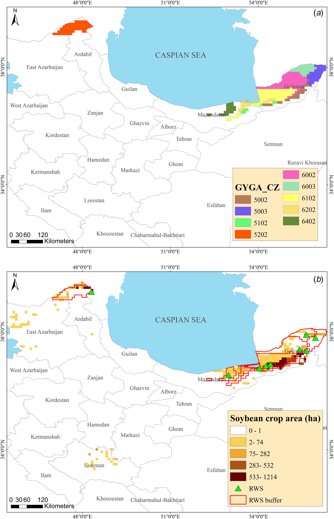
Fig. 1. Colour online. Global yield gap atlas climate zone (GYGA-CZ) which cover 1% or more of the Iran soybeans zone (a), and selected RWS (reference weather station) for soybean cropland use areas with their 100 km buffer zone (b).
Model used
The model used in the current study was SSM-iCrop2 (Soltani and Sinclair Reference Soltani and Sinclair2012; Soltani et al., Reference Soltani, Alimagham, Nehbandani, Torabi, Zeinali, Dadrasi, Zand, Ghassemi, Pourshirazi, Alasti, Hosseini, Zahed, Arabameri, Mohammadzadeh, Rahban, Kamari, Fayazi, Mohammadi, Keramat, Vadez, van Ittersum and Sinclair2020). This model can be downloaded from ‘www.SSM-crop-models.net’. The model includes daily phenology progress, leaf area development and senescence, dry matter production, yield formation and soil water balance. Responses of crop processes to solar radiation, temperature, water availability and cultivar differences are included in the model. Soil water sub-model accounts for soil water additions from precipitation or irrigation, and increasing rooting depth and water removal via deep drainage, run-off, soil evaporation and plant transpiration. The soil profile is divided into two layers: one top layer of 15–20 cm thickness and a second layer that includes the first layer and its depth increases by root growth. Soil water balance of both layers is calculated separately. The effect of water deficit and excess on leaf area development and senescence, dry mass accumulation and phenological development are simulated. The model also accounts for the effect of freezing temperatures on plant leaf area that might take place in early spring sowings or winter sowings. The model has been tested extensively for a wide range of plant species including soybean and proved to be robust (Soltani et al., Reference Soltani, Alimagham, Nehbandani, Torabi, Zeinali, Dadrasi, Zand, Ghassemi, Pourshirazi, Alasti, Hosseini, Zahed, Arabameri, Mohammadzadeh, Rahban, Kamari, Fayazi, Mohammadi, Keramat, Vadez, van Ittersum and Sinclair2020).
Weather data
Meteorological information of each experimental site including minimum and maximum daily temperature, daily precipitation and solar radiation were obtained from the nearest meteorological station. Outliers and missing data were then estimated and restored using the WeatherMan program (Hoogenboom et al., Reference Hoogenboom, Jones, Wilkens, Porter, Batchelor, Hunt, Boote, Singh, Uryasev, Bowen, Gijsman, Dutoit, White and Tsuji2004).
Soil data
The required soil information included soil albedo, drainage coefficient, soil water volumes at the field capacity, wilting point and saturation conditions. There is no local digitized soil database for crop modelling in Iran, so the HC27 database (Koo and Dimes, Reference Koo and Dimes2013) was utilized. The resolution of the soil database is also important. HC27 soil database used in the current study has a resolution of 10 km which may seem coarse; however, tests using SSM-iCrop2 for crop and horticultural species indicated that using HC27 soil profiles compared to actual, measured soil profiles resulted in similar output for yield and the net amount of irrigation water requirements or evapotranspiration with no significant difference with respect to mean, variance and distribution (Nehbandani et al., Reference Nehbandani, Soltani, Naghab, Dadrasi and Alimagham2020a). The detailed soil parameters that were used to reflect each individual soil type into a model are shown in Table 1.
Table 1. The detailed soil parameters based on HC27 soil database (Koo and Dimes, Reference Koo and Dimes2013)

Soil codes (IFPRI Harvest Choice): 2 = clay, high fertility, 120 cm depth; 5 = clay, medium fertility, 120 cm depth; 14 = loam, medium fertility120 cm depth; 17 = loam, low fertility 120 cm depth. SOC, soil organic carbon; SALB, soil albedo; CN2, curve number; DRAINF, drainage factor; SAT, volumetric soil water content at saturation; DUL, volumetric soil water content at drained upper limit; EXTR, volumetric soil water content available for extraction by crop roots.
Crop management data
To run the model, some management information including sowing date and rate, cultivation type (under irrigation or rainfed) and crop's parameters must be entered into the model. Soybean farm management is similar throughout Iran due to the limited crop area. Wheat-soybean double cropping is the common rotation practice in the region. The common sowing date of soybean is early in summer. Therefore, 25th June (176th day of the year) was considered as a fixed sowing date for all stations. The cultivation type was also considered to be irrigated due to the lack of proper rainfall in the growing season. The model used the fraction of transportable soil water (FTSW) threshold to trigger irrigation when the soil water balance detected an FTSW value that was below 0.41. The crop parameters were used in the model extracted from common cultivars of the regions including Katoul, Tellar, JK (Maturity group V, growth period of about 150 days) and Williams (Maturity group III, growth period of about 120 days). Nehbandani et al. (Reference Nehbandani, Soltani, Nourbakhsh and Dadrasi2020b) parameterized and evaluated the SSM-iCrop2 model for soybean cultivars in Iran (values of r, CV and RMSE were obtained at 0.84, 13% and 500 kg/ha, respectively). Therefore, we used their information in the current study. The model was run for the different soil types in each RWS. Then, the average potential yield for a period of 10 years (2005–2014) was calculated for each soil type. Finally, the RWS potential yield was determined using the weighted average according to the area of each soil type.
Quantifying of yield gap causes
To identify the causes of the soybean yield gap, the on-farm data of some survey studies between 2011 and 2016 in the northern part of Iran, which is the main production area of soybean, were selected for analysis using stepwise regression (Draper and Smith, Reference Draper and Smith1998). The diversity of farmers concerning crop yield and management practices is necessary for the success of this analysis. A total of 224 soybean farms were monitored during five growing seasons (2011–2016) while management factors were investigated and recorded (in total, 67 management variables including seedbed preparation, cultivars, nitrogen and phosphorus fertilizer rate, sowing date, seed rate, intra and inter-row spaces, number of irrigations, etc.). In stepwise regression, the studied farms must have all the required information related to considered variables. Therefore, farms even with a lack of one variable in the data set were excluded from the analysis. The data of 138 soybean farms diverse in terms of crop area, management practices and yield were chosen from the data set for further analysis. The relationship between all measured quantitative and qualitative variables (binary numbers for qualitative variables) and yield was investigated through the step-by-step regression method.
Stepwise regression ended up to a regression model with four independent variables. The model was as follows:

where Y is yield (kg/ha), X 1 is the number of irrigations, X 2 is sowing date (days from 1st January), X 3 is the net nitrogen rate (kg/ha) and X 4 is the amount of P2O5 consumed (kg/ha).
Optimization of agronomy practices
To determine the optimal range of factors causing the soybean yield gap (selected by stepwise regression), all the data of 224 soybean farms were used to analyse further using BLA. There is no agreed protocol for the application of BLA, and in some studies, an arbitrary boundary line is fitted to the data (Makowski et al., Reference Makowski, Doré and Monod2007). However, three general steps can be considered to obtain the boundary line (Shatar and McBratney, Reference Shatar and McBratney2004; Makowski et al., Reference Makowski, Doré and Monod2007; Patrignani et al., Reference Patrignani, Lollato, Ochsner, Godsey and Edwards2014; Hajjarpoor et al., Reference Hajjarpoor, Soltani, Zeinali, Kashiri, Aynehband and Vadez2018):
1. Examining the scatter plot of data: a scatter plot (XY chart) should be prepared with crop yield as a dependent variable and one selected management variable (e.g. sowing date or number of irrigation) as an independent variable. This step visualizes the data cloud and facilitates selecting a proper function to be fitted at the data cloud's upper edge.
2. Selection of the data points from the upper edge of the data cloud to be used in the curve fitting: this can be done simply by eye (e.g. French and Schultz, Reference French and Schultz1984) or by an advanced statistical method (e.g. Milne et al., Reference Milne, Ferguson and Lark2006). In the current study, data points from the data's upper edge, the cloud was selected by eye, and an appropriate function was fitted to these points.
3. The final step is to fit a function to the data points obtained from the second stage. This stage results in a model that explains the maximum yield's response to different levels of the independent variable under examination. Parameter estimates of the model can be further used for interpretation.
In the current study, ArcGIS version 10.5 was used to draw maps and SAS version 9.4 (Statistical package) to analyse data applying stepwise regression and BLA methods.
Results
Yield gap estimation and distribution
Ya showed a range of variation from a minimum of 1933 kg/ha in CZ #6003 (coverage = 3%) to a maximum of 2573 kg/ha in CZ #6402 (coverage = 1%) (Table 2 and Fig. 2). For Yp, CZ #5002 (coverage 18%) and CZ #5202 (coverage 10%) with the averages of 5086 and 4232 kg/ha, respectively, had the highest and the lowest Yp. The biggest coverage (30%) belonged to CZ #6102 with Ya of 2346 kg/ha and Yp of 4590 kg/ha. In total, soybean actual yield and potential yield were 2257 and 4681 kg/ha, respectively (Fig. 2). Comparing Yp and Yg indicates that in CZs with higher Yp, the greater is Yg (Fig. 2).
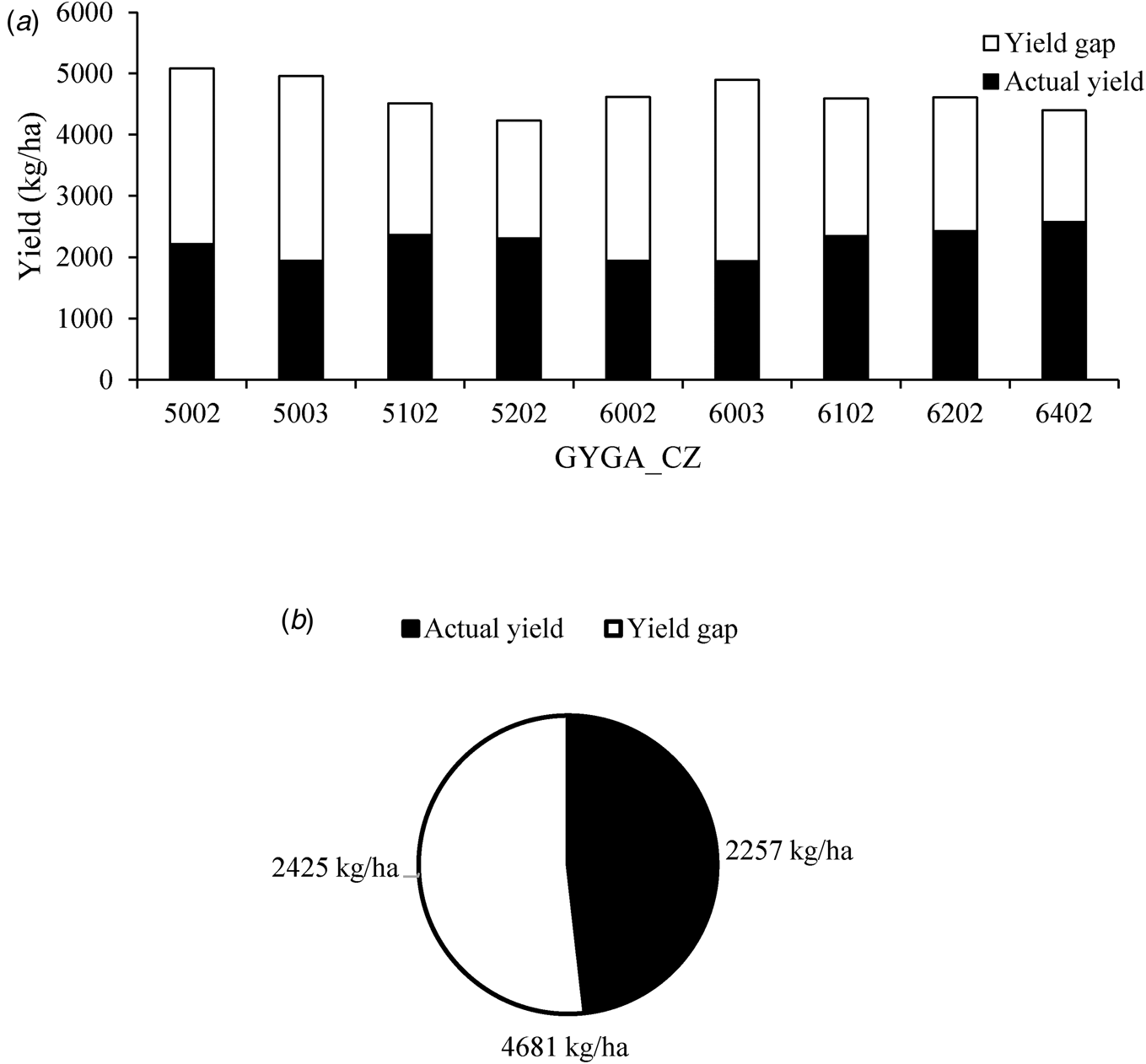
Fig. 2. Summary of actual yield, yield potential and yield gap of soybean for each global yield gap atlas climate zone (GYGA-CZ) (a), and the whole country (b) (www.yieldgap.org/iran).
Table 2. Summary of soybean crop area and soil code for each global yield gap atlas climate zone (GYGA-CZ) and the whole country (www.yieldgap.org/iran)
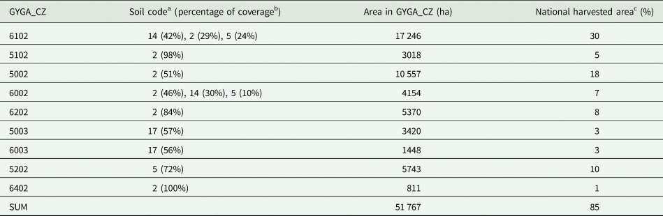
a 2 = Clay, high fertility, 120 cm depth; 5 = clay, medium fertility, 120 cm depth; 14 = loam, medium fertility, 120 cm depth; 17 = loam, low fertility, 120 cm depth.
b Based on GYGA protocol, soil classes were selected until achieving at least 50% area coverage of crop harvested area within RWS.
c In countries with relatively uniform topography, at least 40–50% coverage of total harvested crop area within weather station buffer zones is required for a robust estimate of Yp or Yw at a national level (Van Wart et al., Reference Van Wart, van Bussel, Wolf, Licker, Grassini, Nelson, Boogaard, Gerber, Mueller, Claessens, van Ittersum and Cassman2013).
Quantifying of yield gap causes
The relation of predicted (using equation 1) and observed (on-farms) yield showed that the accuracy of the model (equation 1) is appropriate and can be applied to identify the constraint variables (RMSE = 190 kg/ha, CV = 6 and r = 0.51; Fig. 3). According to this model, the most important soybean yield gap causes were number of irrigations, sowing date, amount of nitrogen consumed and amount of P2O5 consumed.
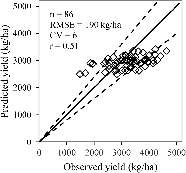
Fig. 3. Predicted yield using a regression model (equation 1) v. observed on-farm soybean yield. The 20% ranges of discrepancy between predicted and observed are indicated by dashed lines. Solid line is 1:1 line.
Optimization of agronomy practices
The minimum, maximum and average irrigation times in the investigated farms were 1, 10 and 5, respectively. However, irrigation recommendation depends on the year of study and the amount of rainfall: applying BLA on 5 years' study data showed that at least five irrigation events (higher than about 300 mm) were required to reach a potential yield of 6076 kg/ha (Fig. 4).
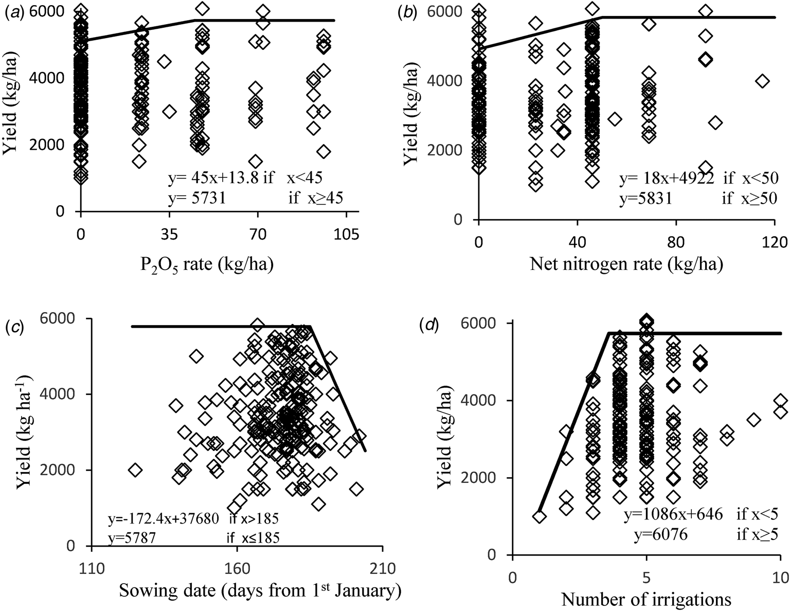
Fig. 4. Distribution of yield values v. net nitrogen rate (a), P2O5 rate (b), number of irrigation (c) and sowing date (d) with fitting function boundary line (the black line on the graph of the function fitted maximum yields).
A two-segmented model was recognized as the boundary line using the data of yield v. total nitrogen fertilizer (Fig. 4). While the range of nitrogen fertilizer consumption in the investigated farm was between 0 and 115 kg/ha, BLA showed that a minimum nitrogen fertilizer of 50 kg N/ha was required to reach a potential yield of 5831 kg/ha (Fig. 4). According to the boundary function, using more than this amount cannot necessarily lead to higher potential unless other factors forming yield would change.
In studied farms, farmers applied a range of phosphorus fertilizer applications between 0 and 96 with an average of 22 kg P2O5/ha. According to the boundary line, soybean yield response to phosphorus fertilizer could also be explained with a two-segmented function (Fig. 4). When applied to phosphorus fertilization, BLA showed a potential yield of 5731 kg/ha that was obtained by consuming at least 45 kg P2O5/ha (Fig. 4).
Soybean sowing dates ranged from the 124th to the 210th day of the year; in other words, 4th May to 29th July. To reach a soybean yield of 5787 kg/ha, sowing must be done earlier than the 185th day of the year, i.e. earlier than 3rd July (Fig. 4).
Discussion
Crop simulation models have been known as one of the best tools to estimate Yp or Yw in yield gap analysis (Lobell, Reference Lobell2013; Van Ittersum et al., Reference Van Ittersum, Cassman, Grassini, Wolf, Tittonell and Hochman2013). Yp simulation illustrated that Yp for the main soybean regions of Iran ranged between 4232 and 5086 kg/ha. The range of simulated yields agrees with the 4430–4860 kg/ha yield-potential range estimates discussed by Nehbandani et al. (Reference Nehbandani, Soltani, Nourbakhsh and Dadrasi2020b), using the same model for Golestan Province, Iran.
According to the stepwise regression analysis, we can argue that soybean yield in Iran was limited mainly by the inefficient use of environmental resources (mainly water, nitrogen, phosphorus and sowing date). In the past decades, much emphasis has been placed on plant genetics and breeding to improve crop yield while seeking the best agronomy practice to close the yield gap has been largely neglected (Soltani et al., Reference Soltani, Hajjarpour and Vadez2016). George (Reference George2014) reported that the focus must shift from relying mainly on germplasm-driven increases in total production to increasing Ya and productivity of inputs through effective agronomy practice. Therefore, searching the best agronomy practice in order to close the yield gap must be brought into the focus.
Our results indicated that 51% of farmers irrigated their farms less than the minimum required irrigation times (five times irrigation). In regions of the world affected by seasonal or chronic water scarcity, yield gap closure is strongly dependent on irrigation (Davis et al., Reference Davis, Rulli, Garrassino, Chiarelli, Seveso and D'Odorico2017). The amount of irrigation water requires for soybean in Iran is 821 mm (Davis et al., Reference Davis, Rulli, Garrassino, Chiarelli, Seveso and D'Odorico2017), while the average rainfall in Iran is 250 mm. Thus, soybean irrigation is inevitable to achieve maximum yield, especially during yield formation. Water stress can also reduce biological nitrogen fixation in soybean (Serraj and Sinclair, Reference Serraj and Sinclair1996).
Among the studied farms, 89% have applied less N fertilizer than optimum requirements (minimum of 50 kg N/ha). It is worth noting that nitrogen addition is not the universal practice in soybean production. Nitrogen biological fixation by symbiotic bacteria provides only 80–90% of the required nitrogen in Iran (Bieranvand et al., Reference Bieranvand, Rastin, Afarideh and Sagheb2003). Soils typically lack Bradyrhizobium japonicum strains unless soybean is grown on them for at least 5 or more years (Solomon et al., Reference Solomon, Pant and Angaw2012). It is consequently important to inoculate seeds with relevant strains of bacteria before sowing, especially if the crop is to be grown for the first time on the land (Solomon et al., Reference Solomon, Pant and Angaw2012). Soybean is not a native species of Iran, and all cultivars are imported. Currently, Katol is the most cultivar used in Iran imported from the USA (dpx3589 genotype). So far, there is no reliable evidence indicating the differences in nodulation among soybean cultivars in Iran. Still, according to the local experts' experience (personal communication), the formation of nodules in Katol cultivar is less than other cultivars. On the other hand, farmers in the major soybean areas of Iran mainly sow soybean without seed inoculation. Suitable strains of bacteria for biological stabilization were not found in soil because soybean is not a native crop in Iran. Therefore, nodules are limited in the plant's roots. Overall, the high dependency of soybean yield on nitrogen fertilizer application in Iran was probably related to the mentioned factors. It is worth mentioning that the above cases need to be studied thoroughly.
In addition to nitrogen, other nutrients (such as phosphorus, potassium, etc.) would also limit crop yields (Hajjarpoor et al., Reference Hajjarpoor, Soltani, Zeinali, Kashiri, Aynehband and Vadez2018). Results showed that 68% of farmers applied less than the optimum amount of required phosphorus fertilizer (minimum of 45 kg P2O5/ha). Phosphorus is a primary nutrient essential for crop growth and development and important for the regulation of various enzymatic activities and constituent for energy transformation (Schulze et al., Reference Schulze, Temple, Temple, Beschow and Vance2006). Thus, phosphorus-deficient soil and low availability impose major restrictions on the vegetative and reproductive growth development of crop (Vance et al., Reference Vance, Uhde-Stone and Allan2003; Zhang et al., Reference Zhang, Liao and Lucas2014). The phosphorus constraint directly decreases photosynthesis through its negative effects on vegetative crop growth of leaf area development and photosynthetic ability per unit leaf area (Vance et al., Reference Vance, Uhde-Stone and Allan2003; Sulieman et al., Reference Sulieman, Ha, Van Schulze and Tran2013). Also, an inadequate supply of phosphorus can affect carbon absorption and distribution between plant shoots and its underground parts (Zhang et al., Reference Zhang, Liao and Lucas2014).
While various studies have reported the positive effect of early sowing date (May and June) on soybean yield, in Iran (Moosavi et al., Reference Moosavi, Akbar, Khaneghah and Moghanlou2011; Aghayari et al., Reference Aghayari, Faraji and Kordkatooli2015 ), results showed that 10% of farmers' sowing dates were after the ideal date (3rd July). It should be noted that soybean in Iran is the second crop in rotation with wheat. Then it is essential to pay attention to the sowing and harvesting dates of wheat to prevent any delay of soybean sowing. The main purposes of earlier sowing are to have suitable moisture conditions and avoid high temperatures (Heatherly and Elmore, Reference Heatherly and Elmore2004). R5 to R6 stage is a crucial period in soybean growth, and early sowing can stimulate early initiation of R5 and lengthen the duration of the R5 through R6 period (Robinson et al., Reference Robinson, Conley, Volenec and Santini2009). Robinson et al. (Reference Robinson, Conley, Volenec and Santini2009) reported that the number of pods per square meter is the most important factor influencing the yield in changing the sowing date. Under favourable weather conditions, early sowing of indeterminate soybean cultivars increases the number of nodes, pods and seeds (Robinson et al., Reference Robinson, Conley, Volenec and Santini2009). Several studies confirmed a reduction in soybean yield due to late sowing (Egli, Reference Egli1993; Egli and Cornelius, Reference Egli and Cornelius2009; Salmeron et al., Reference Salmeron, Gbur, Bourland, Buehring, Earnest, Fritschi, Golden, Hathcoat, Lofton, Miller, Neely, Shannon, Udeigwe, Verbree, Vories, Wiebold and Purcell2014; Boyer et al., Reference Boyer, Stefanini, Larson, Smith, Mengistu and Bellaloui2015).
Conclusion
This study is one of the few studies in which simulation results are integrated with on-farm information to determine the yield gap and find ways to shrink it. Applying three methods (GYGA protocol, Stepwise regression and BLA), three main subjects related to the soybean yield gap in Iran were addressed. The subjects included estimating the yield gap and mapping its distribution, determining its causes and suggesting agronomy practices for yield gap closure. The results showed a soybean Yp of 4681 kg/ha while Ya was around 2257 kg/ha during the same period which implied that farmers gain only half of the Yp by current practices. Bridging the remarkable yield gap revealed in this study (2424 kg/ha yield gap) could help the country's food supply. Moreover, methods used here indicated that irrigation, sowing date, and nitrogen and phosphorus fertilizers were the most important managerial practices/inputs responsible for the gaps and determined the optimal levels of these variables. The management guidelines outlined in the current study will increase soybean production and can play an effective role in ensuring food security along with working on other major crops in Iran.
Financial support
This research received no specific grant from any funding agency, commercial or not-for-profit sectors.
Conflict of interest
None.
Ethical standards
Not applicable.


