1 Introduction
Pension arrangements have moved to the top of the policy-making agenda over the past decade. Particular attention is given to the question how arrangements can be adapted to deal with the ongoing ageing of the population and the costs associated with it. Therefore, many countries have started to move away from unfunded to funded pension arrangements. The latter often take the form of a defined contribution (DC) scheme. Moreover, other countries that already have a substantial funded pension pillar are now shifting away from defined benefit (DB) towards DC funded arrangements. With the decreasing capacity of pension arrangements to share risks among different cohorts, the question also arises whether there exist alternative channels through which such risks can be shared.
In this paper, we investigate intergenerational risk sharing via both private funded pension arrangements and via budgetary policy. The developments described above suggest that budgetary policy may be becoming more important in this respect. Different cohorts of individuals, including cohorts born in the future, participate in a pension fund and contribute to the government's resources as a tax payer. Moreover, different risks affect the various cohorts in different ways. If the incidence of some risk on a specific cohort is relatively large, it is beneficial to this cohort when this risk can be shared with other cohorts. A pension fund allows elderly cohorts to share risks with younger and future cohorts by varying its financial buffer in response to shocks. The government can do this in a similar way by reducing taxes in response to an unexpected bad shock and allowing the public debt to increase, so that the burden on current cohorts is alleviated and future cohorts participate in the absorption of the bad shock through an increase in the taxes paid to service the higher public debt. Exactly the opposite happens in the case of an unexpected good shock. This way, fluctuations in consumption can be smoothed. A breakdown of intergenerational risk-sharing would thus lead to welfare losses. In our analysis, the fundamental source of risk will be financial market risk.
Not all funded pension arrangements are equally good at providing for intergenerational risk sharing. An individual DC (IDC) scheme in its purest form does not admit any risk sharing among its participants, because all the contributions are invested in the participant's own account who receives the entire return, and not more than that, on his contributions. The tendency towards more DC pension funding is likely to reduce the scope for intergenerational risk sharing, which would eventually result in more consumption volatility over one's lifetime. In this paper, we mainly study collective funded systems which, in principle, allow for at least some intergenerational risk sharing. An important question is to what extent budgetary policy can substitute for intergenerational risk sharing via a funded pension arrangement.
We conduct our analysis in the context of a multi-period stochastic overlapping generations (OLG) model with a pay-as-you-go (PAYG) pension pillar, a funded pension pillar and a government. We assume a fluctuation band on both the pension fund's asset-liability ratio, i.e., the so-called ‘funding ratio’, and on the public debt, while allowing for three margins of policy parameter adjustments. These are the pension contribution rate, the indexation of pension entitlements and the adjustment of tax payments. The intensity of the various adjustments is allowed to increase when the funding ratio or public debt gets closer to the boundaries of their fluctuation band.
We obtain the following main results. First, we observe that among the collective schemes the so-called ‘hybrid’ scheme, which combines elements of both defined-contribution and defined-benefit schemes and which allows both contributions and indexation of pension entitlements to respond to funding ratio imbalances, performs strictly better than the collective defined contribution (CDC) scheme, which holds contributions constant, and the DB scheme, which holds indexation constant. This finding may not be so surprising, since the hybrid scheme has an additional degree of freedom. However, it is important to notice that it is optimal to simultaneously deploy adjustments in contributions and indexation. This way, the volatility of consumption during working life and retirement can be better balanced. We also quantify the welfare gain of deploying both instruments. Second, we find that contribution and indexation policies are substitutes, i.e., stronger responses of contributions to funding ratio imbalances require less active responses in indexation, and vice versa. Third, contribution and tax adjustment policies are also substitutes, while indexation and tax adjustment policies are complements. The intensities of different adjustment margins are selected so as to optimally (from a social welfare perspective) spread the adjustment burden to shocks over workers, the retired and future cohorts.
We also explore the role of the tax regime for intergenerational risk-sharing. We consider two tax regimes, namely the ‘tax-exempt-exempt (TEE) regime’, under which pension fund contributions are levied on after-tax income, while the accumulation and pay-out phases are tax exempt, and the ‘exempt-exempt-tax (EET) regime’, under which contributions are levied on before-tax income, the pension wealth accumulation phase is tax exempt, while the benefits themselves are taxed. In fact, most OECD member countries follow at least partly an EET regime (Whitehouse, Reference Whitehouse1999), in which they facilitate or even stimulate the accumulation of pension wealth by making pension contributions tax deductible (up to a certain limit) and taxing the pension benefits. However, some OECD members have a TEE regime.Footnote 1 We show that levying pension contributions on before-tax income yields higher social welfare, because the resulting additional investment in pension wealth earns the equity premium. Effectively, the fund participant takes out a risk-free loan from the government, which is invested in the pension fund asset portfolio and repaid through the taxes on the future pension benefits. For the various pension arrangements under consideration, the social welfare effect of the higher return on the fund's asset portfolio outweighs the effect of the higher consumption volatility under EET.
This paper connects to different strands of literature. First, it relates to the literature on intergenerational risk-sharing. There is already quite a substantial amount of work that studies intergenerational risk-sharing within a funded pension scheme. Examples are Teulings and De Vries (Reference Teulings and De Vries2006); Gollier (Reference Gollier2008); Cui et al. (Reference Cui, De Jong and Ponds2011) and Draper et al. (Reference Draper, Westerhout and Nibbelink2011), who show how a well-designed pension fund improves welfare by allowing for intergenerational risk-sharing. Bovenberg and Mehlkopf (Reference Bovenberg and Mehlkopf2013) review the literature and the main analytical issues involved in this topic. A number of articles study intergenerational risk-sharing in arrangements that combine funded with PAYG pension pillars, as we do in this paper. Examples are Matsen and Thøgersen (Reference Matsen and Thøgersen2004); Borsch-Supan et al. (Reference Borsch-Supan, Ludwig and Winter2006) and Beetsma and Bovenberg (Reference Beetsma and Bovenberg2009). An important difference of the current paper is that, in contrast to these other works, we consider the government's budget as a separate channel for intergenerational risk sharing. In addition, our modelling setup differs substantially from the frameworks of these other papers. For example, we allow for a continuum of hybrid collective funded schemes that range from schemes that rely relatively strongly on contributions as a steering instrument of the fund's financial position, but little on indexation, to funds that rely little on contributions, but strongly on indexation as a steering instrument. Moreover, the strength of the interventions increases more-than-proportionally with deviations of the funding ratio and public debt from their target values.
Second, this paper also relates to the literature on the taxation of pensions. Gordon and Varian (Reference Gordon and Varian1988); Bohn (Reference Bohn1999); Shiller (Reference Shiller1999); Smetters (Reference Smetters2006) and Ball and Mankiw (Reference Ball and Mankiw2007) show that a government holding equity or taxing capital returns can improve welfare. Whitehouse (Reference Whitehouse1999) makes a case for both the TEE and the EET regime, because the return on savings is untaxed and, hence, the consumption – savings decision during the accumulation phase is undistorted. In Huang (Reference Huang2008), no contributions are paid during the pension accumulation phase and the marginal tax rates during work and retirement are identical, implying that the EET and TEE regimes are equivalent. However, Beetsma et al. (Reference Beetsma, Lekniute and Ponds2011) highlight circumstances in which the equivalence breaks down. For example, the marginal tax rate during retirement is typically lower than during working life. Hence, pension savings are more attractive under the EET regime. Furthermore, the government also shares in the asset market risk under the EET regime, thereby benefiting current pension fund participants. Romaniuk (Reference Romaniuk2013) analyses the optimal pension fund portfolio assuming that utility in retirement is maximised. The taxes levied under the TEE regime do not affect utility maximisation, while those under the EET regime do. Again, the equivalence between the two regimes breaks down. In contrast to Romaniuk (Reference Romaniuk2013) we take the composition of the pension fund's investment portfolio as given, while focussing on the role of the various adjustment channels for intergenerational risk sharing and social welfare.
The remainder of this paper is structured as follows: Section 2 lays out the model, while Section 3 presents the parametrisation for the simulations. In Section 4, we discuss our social welfare criterion. We analyse the results of our simulations in Section 5. Because the multi-OLG model assumes that personal (i.e., non-pension) savings are exogenously fixed at zero, otherwise the computational intensity would become unmanageable, in Section 6 we simulate the model assuming only two OLG and endogenous personal savings. We show that qualitatively the main results from the multi-OLG analysis are retained. Finally, in Section 7 we conclude the main text of this paper. Some technical details are found in the Appendix.
2 The model
The model features OLG with identical agents in each generation. Each period a new generation of mass one is born. During the first part of their life individuals’ work, while during the second part they are retired. Retirement benefits are provided by a first pillar that pays a PAYG social-security benefit and a second pillar formed by a pension fund through which individuals channel their savings. Regarding the pension fund, we distinguish between an individual and a collective fund. The former is an IDC fund, to which the individual pays a fixed contribution during his working life and converts his pension assets into an annuity at retirement. The latter is a collective pension fund that indexes pension entitlements during participation. Labour supply is exogenous and normalised to one at the individual level. Hence, the total amount of labour supplied by a working cohort is also one. Relaxing this assumption would make the analysis computationally even more demanding. For the same reason, the retirement age is taken as given by individuals. These are relatively common assumptions in the related literature. The only exogenous risk factor is the return on a risky asset referred to as equity. There are two assets, namely equity and a risk-free asset. Finally, the variables in our model are expressed in real terms.
2.1 Individuals
An individual lives for TD periods in total. An individual born in period ν features utility
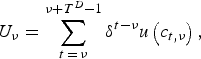 $$U_\nu = \sum\limits_{t \,=\, \nu} ^{\nu + T^D - 1} \delta ^{t - \nu} u\left( {c_{t,\nu}} \right),$$
where δ is the discount factor and c t,ν is consumption. Period utility is given by the constant relative risk aversion (CRRA) function
 $$u\left( {c_{t,\nu}} \right) = \displaystyle{{c_{t,\nu} ^{1 - \rho}} \over {1 - \rho}}. $$
Before retirement the individual receives each period an exogenous wage income of one and he pays a social security tax, while after retirement he receives a PAYG social security benefit. The individual has no personal savings. All his savings are channelled to a pension fund. The current simplified set-up without personal savings proves to be computationally very demanding already. Relaxing this assumption within our multi-OLG set-up would make the analysis computationally prohibitive. In Section 6, we relax this assumption for a two-OLG version of the model and find that the main results of the multi-OLG set-up are preserved.Footnote 2 The assumption here is that individuals are unable to maximise their lifetime utility, because of their limited computational abilities. Nevertheless, they do have specific preferences about the allocation of consumption over time. We could easily assume a positive exogenous rate of personal savings alongside pension savings. However, this would add very little to our analysis. Hence, we assume for convenience that the exogenous personal savings rate is zero.
We consider two different regimes for the taxation of the pension income received from the funded pension pillar. Under the ‘TEE’ regime pension contributions are paid after taxes have been levied on income, while the pension benefits are untaxed. The accumulation of pension wealth is also untaxed. Under this regime, the individual's consumption profile is given by:
 $${c_{t,\nu }} = \left\{ {\matrix{ {1 - \left( {\lambda + {\,p_t} + {\tau _t}} \right),} & {\quad t - \nu \in {\rm \{ }0, \ldots ,{T^R} - 1{\rm \} }} & {({\rm working}),} \cr {\zeta + {\pi _{t,\nu }},} & {\quad t - \nu \in {\rm \{ }{T^R}, \ldots ,{T^D} - 1{\rm \} }} & {({\rm retired}),} \cr } } \right.$$
where λ is the social security tax, p t is the pension contribution, τ t is a tax payment to the government, which is equal for all working generations, TR is the number of working periods, ζ is the social-security benefit and π t,ν is the pension benefit. Retirement thus takes place in period ν + TR. Under the ‘EET’ regime the pension contribution is subtracted from income before taxes are paid, while the pension benefit is taxed. Again, the accumulation of pension wealth is untaxed. In this case,
 $${c_{t,\nu }} = \left\{ {\matrix{ {\left( {1 - {\,p_t}} \right)\left( {1 - {\tau _t}} \right) - \lambda ,} & {\quad t - \nu \in {\rm \{ }0, \ldots ,{T^R} - 1{\rm \} }} & {({\rm working}),} \cr {\zeta + \left( {1 - {\tau _t}} \right){\pi _{t,\nu }},} & {\quad t - \nu \in {\rm \{ }{T^R}, \ldots ,{T^D} - 1{\rm \} }} & {({\rm retired}).} \cr } } \right.$$
2.2 Retirement arrangements
This subsection discusses the details of the retirement arrangements.
2.2.1 The first pillar
Because of the PAYG character of the first pillar, each period total contributions by the working cohorts equal total benefit payments to the retired:
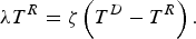 $$\lambda T^R = \zeta \left( {T^D - T^R} \right).$$
2.2.2 The IDC second pillar
The second pillar consists of a pension fund. First, we consider the IDC arrangement and denote by A t,ν the pension asset holdings at the beginning of period t in the IDC scheme. Individuals start with zero initial asset holdings, i.e., A ν,ν = 0. Each period of their working life they add their pension contribution to these asset holdings, which are invested in risk-free debt and risky equity. Hence, the total asset holdings of the individual evolve as,
 $$\matrix{ {{A_{t + 1,\nu }} = \left( {1 + r\,_t^p } \right)({A_{t,\nu }} + \bar p),} & {t - \nu \in \{ 0,...,{T^R} - 1\} } & {{\rm (working)},} \cr } $$
where  $\bar p$ is the contribution paid (at the end of the period) and r tp denotes the return on the asset portfolio, which is given by:
 $$r\,_t^p = (1 - \omega ^p )r\,^f + \omega\, ^p r_t^e, $$
where ωp is the fraction of the pension fund's assets invested in equity, r f is the constant return on the risk-free debt and r te is the return on equity.
At the beginning of retirement (t − ν = TR), the individual converts his pension assets into an annuity a t,ν:
 $$\eqalign{A_{\nu + T^R, \nu} = & a_{\nu + T^R, \nu} \sum\limits_{\,j = 0}^{T^D - T^R - 1} {\displaystyle{1 \over {\left( {1 + \bar r^p} \right)^j}}}, \cr \Rightarrow a_{\nu + T^R, \nu} {\rm} = & {\rm} A_{\nu + T^R, \nu} \displaystyle{{\bar r^p} \over {1 + \bar r^p}} /\left( {1 - \left( {1 + \bar r^p} \right)^{T^R - T^D}} \right),} $$
where  $\mathop {\bar r}\nolimits^p $ is the mean of the net return on the asset portfolio. The subsequent annuity payments are variable and are given by
 $$a_{t + 1,\nu} = a_{t,\nu} \displaystyle{{1 + r_t^p} \over {1 + \bar r^p}}, \quad {\rm for} \ t - \nu \in \{ T^R, {\rm \ldots}, T^D - 2\} \quad {\rm (retired)},$$
This is a variable annuity of the type considered in Feldstein and Ranguelova (Reference Feldstein and Ranguelova1998, Reference Feldstein and Ranguelova2001) and Beetsma and Bucciol (Reference Beetsma and Bucciolforthcoming). It differs from an annuity that pays out the same amount each period. The advantage of the variable annuity is that it allows the individual to take advantage of the equity premium.
The annual pension benefit under the IDC plan is given by:
 $$\pi _{t,\nu} = a_{t,\nu}. $$
2.2.3 The collective second pillar
Let us now turn to the collective pension fund. The advantage of the collective fund is that risks can be shared over many cohorts of participants. Through their contributions into the system, individuals accrue pension entitlements, b t,ν. At the start of the working life, accrued pension entitlements are zero, b ν,ν = 0. Pension entitlements evolve as follows:
 $${b_{t + 1,\nu }} = \left\{ {\matrix{ {(1 + {I_t}){b_{t,\nu }} + \psi ,} & {\quad t - \nu \in \{ 0,{\rm \ldots },{T^R} - 1\} } & {{(\rm working),}} \cr {(1 + {I_t}){b_{t,\nu }},} & {\quad t - \nu \in \{ {T^R},{\rm \ldots },{T^D} - 1\} } & {{(\rm retired),}} \cr } } \right.$$
where I t is the indexation rate and ψ is the accrual. The accrual is received at the beginning of period t, just after the already existing entitlements have been adjusted for indexation. Notice that all participants in the pension arrangement receive the same indexation. This period's pension payouts are done after this period's indexation is applied; that is, the annual pension benefit under the collective pension fund is given by:
 $$\pi _{t,\nu} = (1 + I_t )b_{t,\nu} $$
and total pension payouts of the pension fund
 $$\Pi _t = \sum\limits_{\nu = t - T^D + 1}^{t - T^R} \,\pi _{t,\nu}. $$
The pension fund's assets A t+1 now evolve as:
 $$A_{t + 1} = \left( {1 + r_{t + 1}^p} \right)\left[ {A_t + T^R p_t - \Pi _{t}} \right],$$
where r tp is again the return on the pension fund's asset portfolio. Hence, the new level of pension fund assets is equal to the old level multiplied by the gross portfolio return plus total contribution payments, minus total benefit payments. We assume some given starting level A 0 for the pension fund's assets. For convenience, we can set  $A_0 = \bar A$, the target level of assets to be discussed below. Note that, while contributions are identical for all cohorts in a given period, this is not necessarily the case for the benefits. To facilitate the comparison with the case of the IDC system, we assume that the composition of the fund's portfolio is the same as that of the IDC portfolio. Hence, the return on the pension fund's portfolio is:
 $$r_t^p = (1 - \omega ^p )r^f + \omega ^p r_t^e, $$
where ωp is the fraction of the pension fund's assets invested in equity.
We evaluate the pension fund's liabilities according to the so-called ‘Accumulated Benefit Obligation’ (ABO), which is the discounted sum of all future pension benefits, where its calculation is done under the assumption that the benefit level throughout the retirement period is equal to the current level of accrued entitlements. More specifically, this calculation ignores the further accrual of entitlements by current and future workers through future contributions and the future indexation of entitlements for any current and future participating cohorts. The question is what is the appropriate rate at which those benefits should be discounted. If they are risk-free, they should be discounted at the risk-free rate of interest. However, the indexation rate of the pension rights is stochastic, which makes the cash flows stochastic as well. Risk aversion would justify a higher discount rate. Nevertheless, real-world pension arrangements, like the Dutch second pillar, often use the market risk-free interest rate to calculate pension liabilities. Hence, we use the risk-free rate to discount future pension benefits. Since we assume that the risk-free rate is constant, we can write the discount rate of the current entitlements of a participant with the age of t−ν as
 $${R_{t - \nu }} = \left\{ {\matrix{ {\sum\nolimits_{s = {T^R} - (t - \nu )}^{{T^D} - 1 - (t - \nu )} {{{(1 + {r^f})}^{ - s}}} \quad } \hfill & {t - \nu \in \{ 0,...,{T^R} - 1\}\ {(\rm working),}} \hfill \cr {\sum\nolimits_{s = 0}^{{T^D} - 1 - (t - \nu )} {{{(1 + {r^f})}^{ - s}}} \quad } \hfill & {t - \nu \in \{ {T^R},...,{T^D} - 1\}\ {(\rm retired),}} \hfill \cr } } \right.$$
Therefore, current liabilities L t, before this period's indexation decision and accrual, are given by
 $$L_t = \sum\limits_{\nu = t - (T^D - 1)}^t \,R_{t - \nu} b_{t,\nu}. $$
Rewriting (15) (see Appendix A.1) gives the recursive representation
 $$L_{t + 1} = (1 + r^f )\left[ {(1 + I_t )L_t - \Pi _t + \psi \sum\limits_{t - \nu = 0}^{T^R - 1} {R_{t - \nu}}} \right].$$
The current liabilities consist of the present value of the previous liabilities corrected for indexation, minus the present value of the pension payouts in the previous period corrected for indexation, plus the present value of newly accumulated pension entitlements through the accrual obtained by all working cohorts.
An important input for policy decisions is the so-called ‘funding ratio’, defined as:
 $$F_t = A_t /L_t. $$
Note that this period's funding ratio is defined using the assets and liabilities without this period's indexation and cash flows. The funding ratio is subject to a lower bound Fl and an upper bound Fu. In reality, boundaries on the funding ratio are frequently observed. In the context of the current model, we conjecture that in the absence of such boundaries it would be optimal to not have the fund's steering instruments react at all to the funding ratio. This way, the shocks are spread out over as many generations as possible. However, the funding ratio could then reach very low or very high values that are clearly unrealistic. When it is substantially below one, young cohorts could refuse to continue participating in the pension arrangement, because the contributions they would have to make to restore the fund's financial position would far outweigh the benefit they perceive to obtain when they are themselves old (e.g., see Beetsma et al. (Reference Beetsma, Romp and Vos2012); Chen and Beetsma (Reference Chen and Beetsma2013)). By contrast, when the funding ratio is substantially above unity, old generations could put pressure on the fund's board to dismantle the fund and distribute its assets over the participants (possibly in proportion to the contributions that the various participating cohorts have made in the past; see, for example, Penalva and Van Bommel (Reference Penalva and Van Bommel2011) and Beetsma and Romp (Reference Beetsma and Romp2013)). Alternatively, the government might want to tax some of the fund's reserves away.
The pension fund aims at achieving a target  $\bar F$ for the funding ratio, with
  $\bar F = {\textstyle{1 \over 2}}(F^l + F^u )$, the average of the upper and lower bounds on the funding ratio. These bounds define a proportionality parameter
  $q_F = 1 - F^l /\bar F$ indicating the range over which the funding rate can fluctuate. Based on the actual funding ratio F t, the pension fund applies its steering instruments, namely the pension contribution and the rate of indexation of the pension entitlements.
In response to a deviation of the funding ratio from its target level  $\bar F$, the pension contribution will be adjusted as follows:
 $$p_t = \left[ {1 + g_\alpha \left( {F_t /\bar F} \right)} \right]\bar p,\quad g'_\alpha \left(. \right) \le 0,\quad g_\alpha \left( 1 \right) = 0,\quad g'_\alpha \left( 1 \right) = - \alpha, $$
where  $\bar p$ is a target level for the pension contribution (to be discussed below). For function g α we use the so-called tangent hyperbolic adjustment specification with α ⩾ 0,
 $$g_\alpha \left( {F_t /\bar F} \right) = - \alpha q_F \tanh^{- 1} \left( {\displaystyle{{F_t^ * - \bar F} \over {q_F \bar F}}} \right),$$
where F t* is defined as follows:
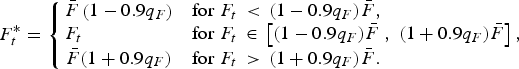 $$F_t^ * = \left\{\matrix{\bar F\left( {1 - 0.9q_F} \right) & {\rm for}\;F_t \, \lt \,(1 - 0.9q_F )\bar F, \hfill \cr F_t \hfill& {\rm for}\;F_t \, \in \,\left[ {(1 - 0.9q_F )\bar F\;,\;(1 + 0.9q_F )\bar F} \right], \hfill \cr \bar F(1 + 0.9q_F ) & {\rm for}\;F_t \, \gt \,(1 + 0.9q_F )\bar F. \hfill} \right.$$
 So if the funding ratio falls below its target ( $F_t < \bar F$), then the pension contribution is raised, and vice versa.Footnote 3 To prevent the adjustment in the contribution rate from reaching extreme values with simulations taking place in discrete time, the adjustment is kept constant as a function of F t when F t approaches its boundaries, i.e., when
 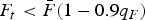 $F_t \lt \bar F(1 - 0.9q_F )$ or
 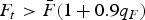 $F_t \gt \bar F(1 + 0.9q_F )$. The reason is that the ensuing discrete-time simulation of the model could lead to values of the funding ratio so close to its boundaries that the adjustment in the contribution rate reaches totally unrealistic levels and produces very sharp movements of the funding ratio in the direction of the opposite boundary. If it were possible to simulate in continuous time this problem would be avoided, because the funding ratio would likely have been pushed back towards its long-run equilibrium value before it could get close to its boundaries. Moreover, the adjustment of the contribution rate would only be short-lived if the funding ratio reaches extreme values. Hence, the current specification ensures smooth adjustment policies for a model that is simulated only at discrete time intervals.
Likewise, the rate of indexation of accumulated entitlements is made a function of the actual funding ratio relative to its target level:
 $$I_t = g_\beta \left( {F_t /\bar F} \right),\quad g'_\beta \left(. \right) \ge 0,\quad g_\beta (1) = 0,\quad g'_\beta (1) = \beta, $$
where for g β we also use the tangent hyperbolic adjustment function with β ⩾ 0, now specified as:
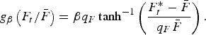 $$g_\beta \left( {F_t /\bar F} \right) = \beta q_F \tanh^{- 1} \left( {\displaystyle{{F_t^ * - \bar F} \over {q_F \bar F}}} \right).$$
Again, the policy intervention is held constant when F t approaches its boundaries.
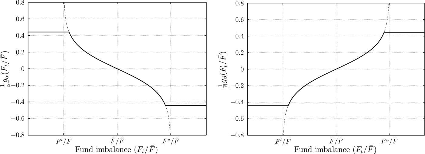
In Figure 1, we graphically illustrate the policies of the pension fund as a function of the funding ratio. In the left panel, we observe that when the funding ratio is below its target, the pension contribution is raised, whereas in the right panel we observe that the indexation of pension entitlements increases if the funding ratio improves. The further the funding ratio moves away from its target, the stronger the policy response. The vertical lines 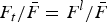 $F_t /\bar F = F^l /\bar F$ and
  $F_t /\bar F = F^u /\bar F$ are the asymptotes of the tangent hyperbolic functions.

Figure 1. Pension contribution adjustment policy (left) and indexation adjustment policy (right) as a function of the target funding level. The dashed lines depict the tangent hyperbolic functions, while the solid lines depict the settings of the policy instruments. Hence, the policy instruments are kept constant when the asymptotes of the hyperbolic tangent function are approached.
2.2.4 Consistency among the targets
To avoid a situation in which pension entitlements need to be systematically revised into one direction, the target levels for the pension contribution, the pension benefit and the funding ratio need to be consistent among themselves. Concretely, in the absence of shocks, and starting from a situation in which all variables are at their target levels, they should be at their target levels in the next period also. For convenience, we refer to this situation as the ‘steady state’. Based on the zero indexation when the funding ratio is at its target  $\bar F$, we have for the pension accrual:
 $$\psi = \bar b/T^R. $$
Hence,
 $$b_{t,\nu} = \left\{{\matrix{{\left( {t - \nu} \right)\bar b/T^R,} & {\quad t - \nu \in \{1,{\rm \ldots}, T^R \}} & {{(\rm working),}} \cr {\bar b,} & {\quad t - \nu \in \{T^R + 1,{\rm \ldots}, T^D \}} & {{\rm (retired)}{\rm.}} \cr}} \right.$$
 The target benefit level  $\bar b$ is a choice variable that determines the scale of the funded pension pillar.Footnote 4 We can substitute these expressions in
  $\bar b$ for b t,ν into Equation (15). This yields a ‘target level’ for the liabilities
  $\bar L$. Given the target for the funding ratio, we obtain the target asset level as
  $\bar A = \bar F\bar L$. Then, using (13), we obtain
  $\bar p$ as:
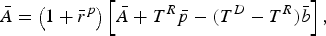 $$\bar A = \left( {1 + \bar r^p} \right)\left[ {\bar A + T^R \bar p - (T^D - T^R )\bar b} \right],$$
where  $\mathop {\bar r}\nolimits^p $ is again the mean of the net return on the pension portfolio. This can be rewritten to
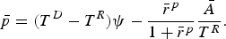 $$\bar p = (T^D - T^R )\psi - \displaystyle{{\bar r^p} \over {1 + \bar r^p}} \displaystyle{{\bar A} \over {T^R}}. $$
We see that the target contribution is increasing in the length of the retirement period TD − TR and the pension accrual, but decreasing in the target asset level and the mean net return on the portfolio.
2.3 The government
In line with the substantial literature studying public debt management (e.g., see the seminal contribution by Lucas and Stokey, Reference Lucas and Stokey1983), the government faces an exogenous stream of primary public spending requirements. We assume that this stream is constant at  $\bar G \ge 0$. As in the aforementioned literature, public spending serves no purpose in terms of providing utility and, since it is exogenous and not an instrument set by the government, it also cannot be used to promote intergenerational risk sharing. However, by setting
  $\bar G$ at a fraction of GDP that is realistic, we can compare different pension arrangements in a quantitatively more meaningful way. In particular, the scope for varying taxes in response to shocks is made more realistic. Taxes can be used to alleviate the shocks that hit individuals in a particular period. When individuals are hit by an adverse shock, taxes can be reduced. This causes an increase in the public debt, implying that future cohorts have to pay higher taxes in order to finance the higher debt-servicing costs. The opposite happens when individuals are hit by a favourable shock. This way public debt is linked to intergenerational risk sharing through an appropriate choice of taxes.
The government further starts off with a given initial debt level D 0. It places its debt on the international capital market. Assuming that it pays off the debt with certainty, it pays the risk-free interest rate on its debt. The dynamics of the debt follow:
 $$D_{t + 1} = (1 + r^{\,f} )\left[ {D_t + \bar G - T_t} \right].$$
Debt at the start of the next period is current debt plus primary government spending minus total tax revenues T, all multiplied by the gross debt return. These total tax revenues depend on the taxation regime. Under the TEE regime, tax revenues are
 $$T_t = \sum\limits_{\nu = t - (T^R - 1)}^t \,\tau _t. $$
In this regime, only the working cohorts pay taxes. Tax revenues are slightly more complicated under the EET regime:
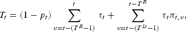 $$T_t = (1 - p_t )\sum\limits_{\nu = t - (T^R - 1)}^t \,\tau _t + \sum\limits_{\nu = t - (T^D - 1)}^{t - T^R} \,\tau _t \pi _{t,\nu}, $$
where total tax revenues are the result of taxing income after the pension contribution has been paid plus the taxation of the pension benefits received by the retired.
The government tries to limit the movements of the public debt by imposing both an upper bound Du and a lower bound Dl on the debt. The upper bound resembles the ceiling that the EU Treaty officially imposes on the public debt. Such a ceiling would prevent the debt from becoming unsustainable. In practice, the main concern is that debt becomes too high, while there seems to be little concern about debt becoming too low. However, this may be the consequence of the fact that debt levels have mostly been substantially larger than zero in recent history. Yet, there are also disadvantages to low or negative debt. For example, financial markets would find it difficult to determine equilibrium interest rates if there is very little debt to be traded, while if debt even becomes negative, hence the government becomes a net creditor, the question is in which assets the government should invest. Moreover, being a large creditor, the government may be held hostage in its policies by its debtors.Footnote 5 In line with these arguments, we assume that besides an upper bound there is also a lower bound on the public debt. The government aims at achieving a target level  $\bar D$ on its debt, with
 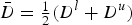 $\bar D = {\textstyle{1 \over 2}}(D^l + D^u )$.
Obviously, this way of modelling budgetary policy is a simplification of reality. Governments often use deficit finance in a variety of alternative ways and for a variety of alternative reasons, such as to mitigate recessions and for public investment. In particular, deficits and debt may respond to political pressures for more spending and less taxation, thereby becoming excessive. As a result, tax revenues would need to be primarily devoted to servicing the public debt and the leeway to use budgetary policy to promote intergenerational risk sharing would be undermined. Political risk may in addition have direct adverse effects on interest payments by the government, thereby further undermining the scope for such policy. However, explicitly taking account of these important and realistic considerations in our model would be beyond the scope of this paper. Hence, here we abstract from these phenomena and focus on the potential for the government to contribute to intergenerational risk sharing, realising that in practice there may be constraints limiting the scope intergenerational risk sharing.
Under the above assumptions taxes are determined by:
 $$\tau _t = \bar \tau \left[ {1 + g_\gamma \left( {D_t /\bar D} \right)} \right],\quad g'_\gamma \left(. \right) \ge 0,\quad g_\gamma (1) = 0,\quad g'_\gamma (1) = \gamma, $$
where γ ⩾ 0 and  $\bar \tau $ is the target tax rate given by
 $$\bar \tau = \left\{{\matrix{{\left( {\displaystyle{{r^f} \over {1 + r^f}} \bar D + \bar G} \right)/T^R} & {\quad {\rm if}\;{\rm TEE,}} \cr {\left( {\displaystyle{{r^f} \over {1 + r^f}} \bar D + \bar G} \right)/\left[ {(1 - \bar p)T^R + (T^D - T^R )\bar \pi} \right]} & {\quad {\rm if}\;{\rm EET}{\rm.}} \cr}} \right.$$
 The target tax rate is the tax rate consistent with permanently keeping debt at its target level  $\bar D$. The target tax rates differ between the TEE and EET regimes, as the government's tax revenues are different under the two regimes. Under the EET regime, the total tax revenues are the sum of the revenues of taxing wage income after the pension contributions have been paid, i.e.,
  $T^R (1 - \bar p)$, and the revenues of taxing retirement income, i.e.,
  $(T^D - T^R )\bar \pi $, while total tax revenues under the TEE regime are obtained by taxing the gross wages of all working generations TR. Similar to the case of the pension fund, we focus on the tangent hyperbolic specification for debt stabilisation,
 $$g_\gamma \left( {D_t /\bar D} \right) = \gamma q_D \tanh^{- 1} \left( {\displaystyle{{D_t^ * - \bar D} \over {q_D \bar D}}} \right),$$
with 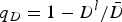 $q_D = 1 - D^l /\bar D$ a measure of how much government debt is allowed to fluctuate. This implies that the tax rate equals its target level if debt also equals its target level. Furthermore, to prevent the tax rate from achieving extreme values, we apply a cut-off to D t* when debt approaches its boundaries. Hence, D t* is given by
 $$D_t^ * = \left\{\matrix{\bar D\left( {1 - 0.9q_D} \right) & {\rm for}\;D_t /\bar D\, \lt \,1 - 0.9q_D, \hfill \cr D_t \hfill& {\rm for}\;D_t /\bar D\, \in \,\left[ {1 - 0.9q_D, 1 + 0.9q_D} \right], \hfill \cr \bar D\left( {1 + 0.9q_D} \right) & {\rm for}\;D_t /\bar D\, \gt \,1 + 0.9q_D. \hfill} \right.$$
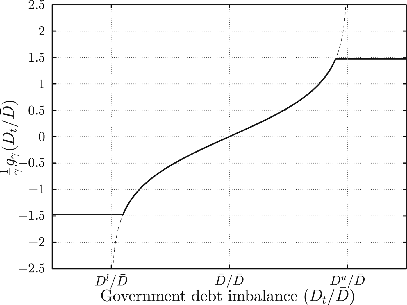
 Figure 2 graphically illustrates that when debt moves away from its target, the deviation of the tax rate from its target becomes larger. The vertical lines  $D_t /\bar D = D^l /\bar D$ and
  $D_t /\bar D = D^u /\bar D$ are the asymptotes of the tangent hyperbolic function.
Figure 2. Tax adjustment as a function of the public debt. The dashed line depicts the tangent hyperbolic function, while the solid line depicts the adjustment of taxes relative to their target as a function of the public debt relative to its target. Taxes are held constant when the asymptotes of the hyperbolic tangent function are approached.
3 Parametrisation
We set the parameters for the individual's life cycle as follows. Each generation starts working at the age of 25, retires at the age of 65 (hence, TR = 40) and dies at the age of 85 (hence, TD = 60). Hence, we follow each generation over a period of 60 years. We set the annual return on the risk-free asset at r f = 2% and assume that the gross return on equity 1 + r te is log-normally distributed with expected equity premium 3% and standard deviation 15%.Footnote 6 Hence, the gross return on equity is distributed as 1 + r te ~ logN(μe,σe) = logN(0.0387, 0.1421).
In view of the absence of capital as a production factor, we calculate GDP as aggregate labour income. Therefore, given that each cohort is of size unity and that labour income is unity, the GDP level is 1*TR. The target debt level is set at 30% of GDP and q D = 1. Therefore, the lower and upper boundaries Dl and Du on the debt correspond to 0% and 60% of GDP, respectively. This choice of the debt upper bound is in line with the institutional framework of the European Union, where the Stability and Growth Pact uses a reference value for the maximum debt-GDP ratio of 60%. Furthermore, government spending is set constant at  $\bar G = 33.33\% $ of GDP. The social security benefit is set constant at ζ = 20%, which implies a social security tax of λ = 10%, because the length of retirement is half the length of working life and no one dies prematurely.
Furthermore, the target funding ratio is  $\bar F = 100\% $ and q F = 0.3, implying funding ratios between 70% and 130% of the target level. We set the fraction of the pension fund's assets invested in equity at ωp = 0.50. The pension contribution and the accrual rate are chosen such that the consumption levels are constant over the lifetimes of individuals in the absence of shocks. With δ(1 + rf) = 1 this is the optimal time profile for consumption in the absence of shocks. Hence, under the TEE regime we choose our parameter values such that
  $1 - \left( {\lambda + \bar p + \bar \tau} \right) = \zeta + \bar \pi $ and under the EET regime such that
  $\left( {1 - \bar p} \right)\left( {1 - \bar \tau} \right) - \lambda = \zeta + \left( {1 - \bar \tau} \right)\bar \pi $.
Table 1 summarises the choices of the parameters. Furthermore, with the above inputs we can calculate steady states for the various regimes. For IDC under the EET regime we have  $\bar p = 0.0830$,
  $\bar \tau = 0.2915$ and
  $\bar a = 0.4936$ the steady-state annuity level. Hence, steady-state consumption is
  $\left( {1 - \bar p} \right)\left( {1 - \bar \tau } \right) - \lambda = \zeta + \left( {1 - \bar \tau } \right)\bar a = 0.5497$. For the IDC under the TEE regime, we find that
  $\bar p = 0.0519$,
  $\bar \tau = 0.3392$ and
  $\bar a = 0.3089$; hence steady-state consumption is
  $1 - \left( {\lambda + \bar p + \bar \tau } \right) = \zeta + \bar a = 0.5089$. For the collective EET regime we find that ψ = 0.0128,
  $\bar A = \bar L = 225.2391\!$,
  $\bar p = 0.0665$ and
  $\bar \tau = 0.2850$. Hence, steady-state consumption is
  $\left( {1 - \bar p} \right)\left( {1 - \bar \tau} \right) - \lambda =$
 $\zeta + \left( {1 - \bar \tau} \right)\bar b = 0.5675$. Finally, for the collective TEE regime, we obtain ψ = 0.0080,
  $\bar A = \bar L = 140.0004$,
  $\bar b = 0.3194$,
  $\bar p = 0.0414$ and
  $\bar \tau = 0.3392$. Hence, steady-state consumption is
  $1 - \left( {\lambda + \bar p + \bar \tau} \right) = \zeta + \bar b = 0.5194$.
Table 1. Choice of parameter values
4 Social welfare evaluation
We simulate N = 10,000 paths for the equity returns and we assume that the economy is in its steady state at time t = 0. There are hardly any policy parameter adjustments close to time t = 0. Hence, we evaluate the simulation results after a ‘burn-in’ period of 100 years, i.e., from time t = 100 onward. This burn-in period is intended to converge to the long-run distribution of our state variables around their steady-state values and to start the recording of our simulation results from there. Given the initial values (A 0, L 0, D 0), there is a hardly any consumption volatility in the first 30–40 periods, because the public debt and the funding ratio absorb the first shocks. Hence, social welfare would be overestimated without the burn-in period. We evaluate the risk-sharing arrangements provided by the government and the pension fund in terms of social welfare. Social welfare evaluated at time t = 100, SW, is the sum of the expected discounted utilities of future generations ν ⩾ 100,
 $$SW = \displaystyle{1 \over N}\sum\limits_{n = 1}^N \,\left( {\sum\limits_{\nu = 100}^\infty \,\delta ^{\nu - 100} U_{\nu, n}} \right),$$
where U ν,n is the utility of the cohort born in period ν of simulation run n. The discounted utility of the generation born in period ν converges to zero as ν goes to infinity. Therefore, we simulate paths of 1,000 periods and truncate the sum in the above expression accordingly. The subsequent discounted utility flows will be negligible in their contribution to social welfare. To ease the welfare comparison of different arrangements, we calculate the certainty-equivalent consumption level (CEC), which is the constant consumption level over the entire lifetime of all future generations ν ⩾ 100, such that social welfare under this constant consumption level is identical to the social welfare level SW calculated from the simulations. Hence, CEC is calculated from
 $$SW = \sum\limits_{\nu = 100}^\infty \,\sum\limits_{t = 0}^{T^D - 1} \,\delta ^{t + \nu - 100} u(CEC).$$
Appendix A.2 shows that
 $$CEC = \mathop {\left( {\displaystyle{{SW(1 - \rho )(1 - \delta )^2} \over {\left( {1 - \delta ^{T^D}} \right)}}} \right)}\nolimits^{{\textstyle{1 \over {1 - \rho}}}}. $$
Direct comparison of social welfare levels between scenarios is not very informative about the quantitative consequences of switching from one policy scenario to another. By contrast, the ratio of CEC levels for two scenarios A and B yields the per cent increase in the constant consumption level over the lifetimes of all current and future cohorts that is needed to raise social welfare in scenario B to that in scenario A.
5 Simulation results
This section discusses the outcomes of our simulations. First, we discuss the results for the individual pension scheme. Second, we investigate the various collective pension arrangements and explore the effects of varying the hyperbolic adjustment policies. Third, we derive socially optimal combinations of risk-sharing parameters under different policy regimes.
5.1 Individual Defined Contribution
As we abstract from wage uncertainty, there are no fluctuations in tax revenues under the TEE regime, implying constant government debt and thus constant tax rates. However, under the EET regime, because the annuity payments are subject to financial market uncertainty and they are a source of tax revenue, both the tax rate and the government debt fluctuate. Although the funded pension pillar cannot provide for intergenerational risk sharing under IDC, the government does promote intergenerational risk sharing by allowing the tax rate to respond to shocks and let fluctuations in tax revenues feed into the public debt. For high values of the tax adjustment parameter γ, even a small deviation of the government debt from its target value results in substantial tax adjustments. For low values of γ, most of the adjustment takes place when government debt is close to its boundaries. Our simulations show that for γ below 0.15, the tax adjustments are too small, such that the government debt may cross its boundaries. Hence, we confine ourselves to γ ⩾ 0.15. Under this restriction, social welfare under IDC is maximised at γ = 0.85. For this value of the tax adjustment parameter risks that occur at any moment are optimally spread over current and future cohorts. For the remainder of this paper, we take 0.85 as our benchmark value of γ when we hold it constant.
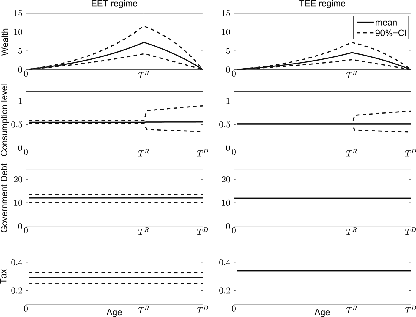
Figure 3 shows the mean simulation paths and the 90% confidence intervals around those means for the IDC pension arrangement under both taxation regimes. The welfare levels in terms of CEC are 0.5282 and 0.4948 under the EET and TEE regimes, respectively. Compared to the TEE regime, the advantage of the EET regime is that individuals can invest the tax savings during their working life in a portfolio that contains a mix of risk-free debt and equity. While consumption volatility is lower under TEE, the effect of higher average consumption under EET dominates this disadvantage in terms of the effect on social welfare.
Figure 3. Life cycle dynamics for an IDC pension scheme under EET and under TEE. The graphs depict for the two types of tax regimes the simulated mean (solid line) and 90% confidence interval (dashed lines) of the relevant variables as a function of age. These graphs are drawn for the optimal tax adjustment parameter (γ = 0.85).
5.2 Collective funded pension arrangements
Recall that we have set accrual such that the steady-state consumption is constant over life. Table 2 summarises the steady-state values of the variables that we computed earlier.
Table 2. Steady-state values for collective funded pension arrangements
5.2.1 Varying the boundaries on government debt and the funding ratio
This subsection explores how the width of the bands on the government debt and the funding ratio affect social welfare. We consider the EET regime first. The pension fund's investment portfolio is the source of risk, which is eventually shared between the current and future fund participants through different channels. Current participants absorb part of the risk via adjustments in indexation and/or their pension contribution, while future participants absorb part of the risk by letting the funding ratio and the public debt vary between their boundaries. Figure 4(a) shows the welfare effects of varying these boundaries under the EET regime. We set α = 5 and β = 0.5. These are intermediate values for the contribution and indexation policies as we will observe in Section 5.2.2 below, where we study the variations in the instrument settings in more detail. Welfare, as measured in terms of certainty-equivalent consumption, rises if the bands on the funding ratio and the debt level become wider. A wider band on the funding ratio means that the indexation rate can be kept more stable, allowing for a more stable retirement income. Similarly, a wider band on the debt–GDP ratio means that the government has more freedom to set the tax rate so as to shift the effects of shocks to future periods, thereby stabilising after-tax income. In effect, wider bands on the funding ratio and the public debt level allow for more intergenerational risk-sharing. However, the welfare effects of widening these fluctuation margins are rather small. For q F = 0.2 and q D = 0.25, CEC is 0.5425, while for q F = 1.5 and q D = 3, which implies a substantial widening of both fluctuation margins, CEC rises to 0.5430. Under the TEE regime, the government does not absorb any of the uncertainty and, therefore, the debt ratio is stable. Hence, changing the band on the debt does not affect welfare. Panel (b) of Figure 4 shows that widening the band on the funding ratio also raises social welfare under the TEE regime, but the effect is again rather small. Raising q F from 0.2 to 1.5 lifts CEC by about 0.05%.
Figure 4. The figure depicts CEC of social welfare when varying the boundaries on public debt and the funding ratio under the EET regime (left) and TEE regime (right). The simulations are based on α = 5, β = 0.5 and γ = 0.85.
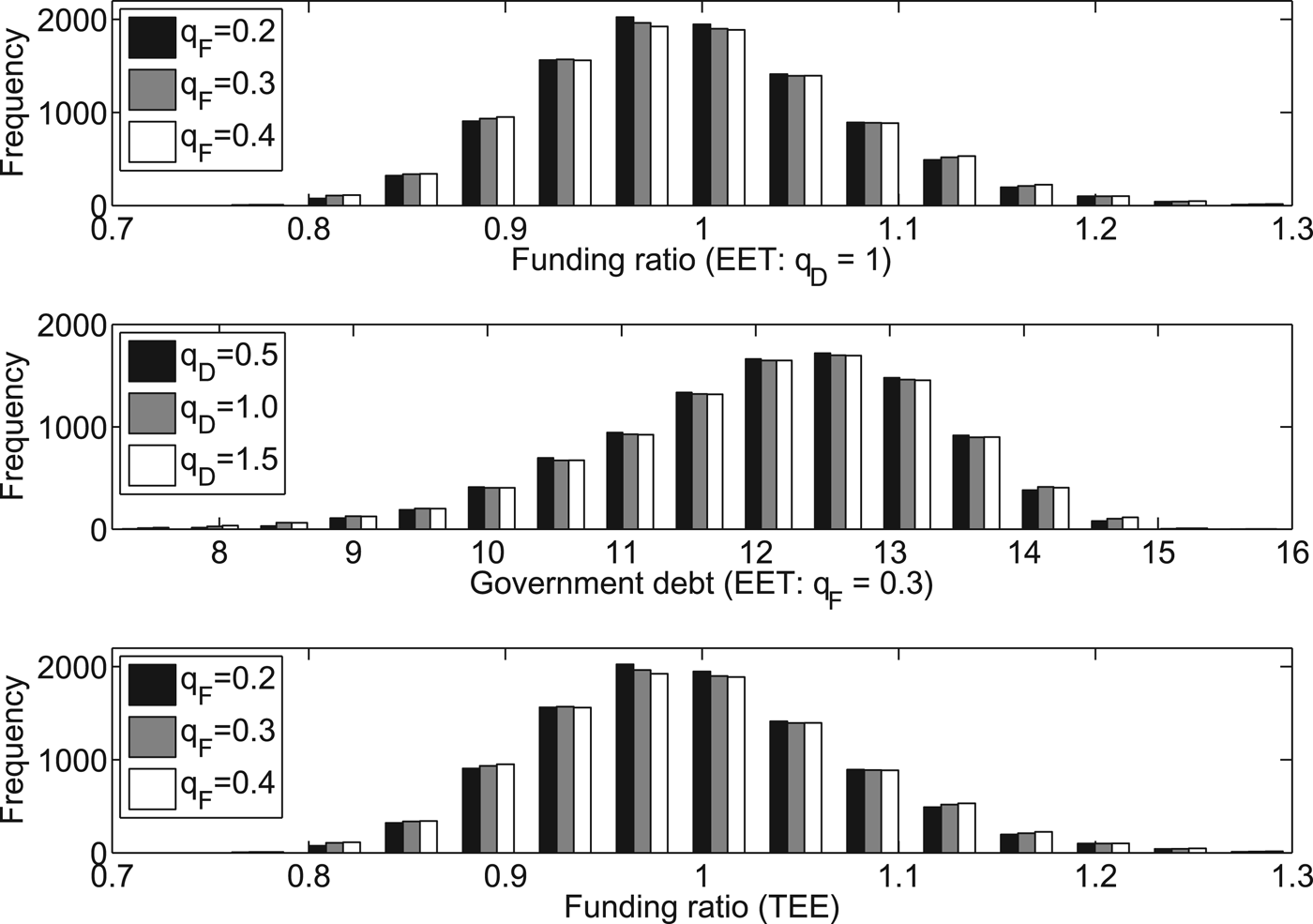
The question is what causes a widening of the bands on the funding ratio and the public debt to have such small welfare effects. Figure 5 shows the frequencies of the funding ratio and the government debt at time t = 100 based on N = 10,000 simulation runs. The figure suggests that the small welfare effects can be explained by the low chances of being close to the boundaries. In fact, a widening of the boundaries on the funding ratio and on the public debt has only marginal effects on the frequency distributions. The skewness in the frequency distributions is the result of the assumption of a log-normal distribution for the equity returns, which is positively skewed.
Figure 5. Frequency distributions of funding ratio and government debt at end of burn-in period. The simulations are based on α = 5, β = 0.5 and γ = 0.85.
For the remainder of this section we assume that the boundaries on the funding ratio and government debt are given. Specifically, we set these boundaries again at the benchmark values corresponding to q F = 0.3 and q D = 1.
5.2.2 Collective funded pension arrangements
We will now study collective funded pension schemes. A special case is the CDC scheme, which features a fixed contribution rate, i.e., α = 0, and a variable pension benefit. Imbalances in the funding ratio will be restored through indexation policy only. Another special case is the DB scheme, which is obtained by setting β = 0. In this case, fund imbalances are restored through adjustments in the contribution only, while the retirement benefits are constant, as there is no (risky) indexation. Finally, arrangements that allow both contributions and indexation to be adjusted, i.e., α, β > 0, will be referred to as hybrid schemes.
In our simulations, we need to impose some restrictions, because we have to hold policy variables constant when the relevant tangent-hyperbolic function reaches its asymptotes. As a result, explosive behaviour of the funding ratio cannot be excluded a priori. First, given a low value of the indexation parameter β, a low value of α results in extremely volatile funding ratios and occasional contribution hikes that would produce negative consumption for workers. Hence, for the DB scheme (β = 0), we set α ⩾ 12, while for the CDC and hybrid schemes, we set β ⩾ 0.2.
Figure 6 shows CEC for different combinations of adjustment policies. Panels (a)–(d) consider the EET regime, while panel (e) considers the TEE regime. Figure 6(a) shows social welfare under CDC for different combinations of the indexation parameter β and the tax adjustment parameter γ. The concavity of utility requires the stabilisation burden to be spread as much as possible over all cohorts. For given γ, when β is low, the burden of adjustment in response to shocks is disproportionately on future pension fund participants, hence a further reduction in β lowers social welfare. By contrast, when β is high, the adjustment burden falls disproportionately on the current fund participants; hence a further increase in β also leads to a reduction in social welfare. The optimal value of β trades off these two effects and is found in between these extremes (the truncation of the parameter space may obscure the observation of the internal optimum). Similar arguments explain the existence of an internal optimum for γ when β is held constant. To obtain a sense of the magnitude of the social welfare effect of changing the policy parameters, we observe that going from the lowest social-welfare level depicted in the graph, which is attained at (β, γ) = (0.20, 1.1), to the highest level, which is attained at (β, γ) = (1.45, 0.75), implies an increase in CEC of 1.5%.
Figure 6. The figure depicts CEC of social welfare for combinations of two adjustment parameters, each time holding constant the other adjustment parameter. It does this for different funded pension arrangements and different taxation regimes.
Figure 6(b) shows welfare when also pension contributions are employed to stabilise the funding ratio (α = 5). The increased stability of the funding ratio reduces the uncertainty transmitted to future cohorts and allows a reduction in the indexation adjustment parameter β, this way shifting some of the adjustment burden back to these cohorts. Indeed, the optimal value of β falls compared to when α = 0. The optimal tax adjustment policy depends on the indexation policy. For high values of β, retirement income and, hence, tax revenues tend to be volatile. Effectively, a higher value of β implies that a larger amount of equity risk is initially borne by the elderly and this is transmitted to future cohorts through changes in the public debt. Optimal rebalancing of the adjustment burden across the various cohorts requires this effect to be mitigated through an increase in the tax adjustment parameter γ. Also, in this way, current workers take over some of the additional equity risk falling on the other cohorts. Figure 6(b) shows that for low β the optimal γ is low, while for high β the optimal γ is also high. In other words, the indexation adjustment and tax adjustment policies are complements of each other.
Figure 6(c) holds the indexation parameter β constant, while the contribution adjustment parameter α and the tax adjustment parameter γ are allowed to vary. Holding γ constant, there is an internal optimum in α. Too low values of α would shift too much of the stabilisation burden to the elderly and future cohorts, while too high values of α would disproportionally burden current workers. Similarly, there is an internal optimum for γ when α is held constant: too low values of γ imply debt absorbing too much of the uncertainty with too adverse consequences for the welfare of future cohorts, while high values of γ make current cohorts absorb a too large fraction of the adjustment burden. Furthermore, when α is lower, contributions and, hence, disposable income of workers are more stable, implying that a more active debt stabilisation policy is needed to rebalance some of the adjustment burden away from future cohorts. If α increases, the optimal γ falls, and vice versa. In other words, contribution adjustment and debt stabilisation policies are substitutes.
Figure 6(d) considers the case in which the tax adjustment parameter is held constant. For given β, there is an internal optimum in α, while for given α there is an internal optimum for β. The need to spread the stabilisation burden as much as possible over all current and future generations implies that the optimal value of β falls when α rises, while the optimal value of α falls when β increases. Hence, also contribution and indexation policies act as substitutes in spreading risks across cohorts. Qualitatively speaking, Figure 6(d) is replicated under the TEE regime – see Figure 6(e).
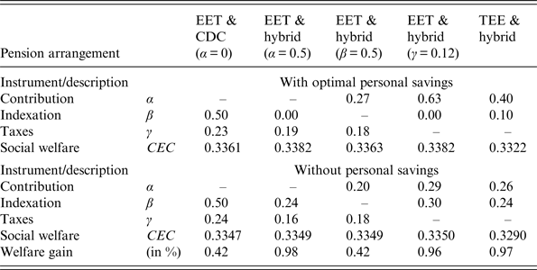
5.3 Social welfare comparison
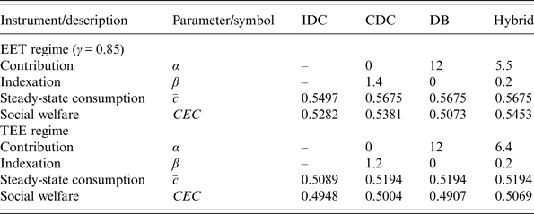
In this section, we compare different tax and pension regimes in terms of social welfare. Again, the tax adjustment parameter is set at its optimum under IDC, i.e., γ = 0.85. The socially optimal parameter settings under the different pension regimes and the corresponding welfare levels in terms of CEC are reported in Table 3. Given the restriction β ⩾ 0.2, the optimal instrument settings under the hybrid regime are (α, β) = (5.5, 0.2) under EET and (α, β) = (6.4, 0.2) under TEE. Under DB, the optimal contribution parameter is at the border of the admitted region, i.e., α = 12, while CDC does yield an internal optimum for indexation of β = 1.4 and β = 1.2 under EET and TEE, respectively. Under both tax regimes, the highest welfare level is obtained under the hybrid pension scheme and the lowest welfare level is obtained under the DB scheme, while the performance of CDC lies in between. That the hybrid regime performs best is not surprising. However, it is important to notice that it performs strictly better than the other two regimes, because this implies that there is a simultaneous stabilisation role both for pension contributions and indexation of pension entitlements. Moreover, the improvement of the hybrid scheme over the other two schemes is quite substantial. Under EET, in terms of CEC the hybrid scheme improves the DB and CDC schemes by 7.5% and 1.3%, respectively, while under TEE it improves the DB and CDC schemes by 3.3% and 1.3%, respectively. Clearly, the largest gain results from adding indexation to the set of policy instruments. We also observe that, for each of the regimes under consideration, EET performs better than TEE. As already explained in Section 5.1, steady-state consumption levels are higher under EET than under TEE, because by postponing taxation individuals can gain from additional investment returns. In terms of social welfare, at the given degree of risk aversion this benefit dominates the effect of higher consumption volatility under EET in comparison to TEE – see Figure 7, which shows for the lifetime consumption of generation ν = 100, the 90% – confidence bands on consumption. Finally, we observe that the collective pension scheme outperforms the individual scheme, but only when indexation policy can be employed to share risks, a result also obtained by Cui et al. (Reference Cui, De Jong and Ponds2011). The comparison with the individual scheme needs to be interpreted with some care, however, because the collective scheme already has a substantial amount of assets when a participant enters, while under the individual scheme the participant starts with zero wealth at entrance.
Figure 7. Life cycle consumption profiles for generation ν = 100 under different regimes. The figures depict the mean (solid line) and 90% confidence interval (dashed lines) of consumption as a function of age.
Table 3. Performance of policy regimes under optimal parameter settings. Instrument parameters are set optimally for the indicated policy regime
6 Two cohort-OLG with personal savings
So far, we have abstracted from personal savings, i.e., voluntary savings outside the pension system. This section explores how the results obtained so far are affected if we allow individuals to optimally choose the level of their savings and its allocation over risk-free and risky assets.
However, first we need to discuss some caveats. To keep the analysis numerically tractable, we simplify the model used thus far by assuming that there are only two overlapping generations at each moment: one active generation and one retired generation. This implies that one period represents a longer time-span than in our multi-period OLG model. Here, we have to compromise between two forces at play. One generation would typically be 30 years. But, since policies are only updated once a period, a period of 30 years would imply that the relative magnitude of a shock would be so large that the funding ratio would be mostly outside its band. This would render an analysis of the welfare effects of adjustment policies infeasible. Therefore, we assume one period to be 5 years. This is longer than in the model without private savings, but still short enough to allow for relatively frequent adjustments of the pension parameters to economic shocks.
The analysis in this section is intended to assess the implications of assuming that personal savings are exogenous at zero. Further research is needed for a fully fledged assessment of the model in the presence of voluntary savings.
6.1 The individual's savings problem
Individuals live for two periods. They work in the first period of their life and are retired in the second period of their life. Hence, at the start of his life an individual born in period ν features utility in Equation (1) with TR = 1 and TD = 2. The individual's budget identities are
 $$\eqalign{A_{\nu, \nu} ^\omega + A_{\nu, \nu} ^{rf} + c_{\nu, \nu} &= 1 - \lambda - \tau _\nu - p_\nu, \cr c_{\nu + 1,\nu} &= A_{\nu, \nu} ^{rf} \left( {1 + r^f} \right) + A_{\nu, \nu} ^\omega \left( {1 + r_{\nu + 1}^e} \right) + \pi _{\nu + 1} + \zeta,} $$
under TEE and
 $$\eqalign{A_{\nu, \nu} ^\omega + A_{\nu, \nu} ^{rf} + c_{\nu, \nu} &= (1 - p_\nu )(1 - \tau _\nu ) - \lambda, \cr c_{\nu + 1,\nu} &= A_{\nu, \nu} ^{rf} (1 + r^f ) + A_{\nu, \nu} ^\omega \left( {1 + r_{\nu + 1}^e} \right) + (1 - \tau _{\nu + 1} )\pi _{\nu + 1} + \zeta,} $$
under EET, where Aω denotes personal risky assets and Arf denotes personal risk-free assets.
The individual maximises expected utility subject to the budget identities by choosing Aω and Arf. The first-order conditions for an internal optimum are
 $$u^{\prime}({c_{\nu ,\nu }}) = \delta (1 + {r^f}){E_\nu }\left[ {u^{\prime}({c_{\nu + 1,\nu }})} \right],$$
 $$\hskip7pt u^{\prime}(c_{\nu, \nu} ) = \delta E_\nu \left[ {\left( {1 + r_{\nu + 1}^e} \right)u^{\prime}(c_{\nu + 1,\nu} )} \right].$$
6.1.1 Retirement arrangements
Because the retired and active populations are of equal size, the social security benefit equals the social security tax. Hence, Equation (5) implies that λ = ζ.
Also, the collective second pillar becomes simpler. Because individuals are born with zero pension entitlements, Equation (11) implies that b ν+1,ν = ψ at the start of retirement. Hence, the annual pension benefit is given by:
 $$\pi _t = (1 + I_t )\psi. $$
The fund's only liabilities are the entitlements of the retired cohort. Hence, Equation (15) reduces to
 $$L_t = \psi. $$
The fund's assets evolve according to
 $$A_{t + 1} = \left( {1 + r\,_{t + 1}^p} \right)\left[ {A_t + p_t - (1 + I_t )\psi} \right].$$
 With zero indexation in the ‘steady state’, the steady-state pension contribution  $\bar p$ obeys:
 $$\bar A = \left( {1 + {\bar r}\,^p } \right)\left[ {\bar A + \bar p - \psi } \right].$$
 Hence, for  $\bar F = 1$ we obtain
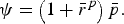 $$\psi = \left(1 + \bar{r}^p \right)\bar{p}.$$
6.1.2 Parametrisation
With two OLG only, some of the parameters need to be adjusted. We assume that one period represents n = 5 years. This is a much shorter time-span than the more realistic assumption that one period (a full generation) is in the range of 20–40 years. However, this is required for our analysis, as explained in the beginning of this section. The risk-free rate becomes 1 + rf = 1.02n and the subjective discount factor becomes δ = 1/1.02n. The density of the gross equity return becomes  $1 + r_t^e \sim \log N\left( {n * \mu ^e, \;\sqrt n * \sigma ^e} \right)$.
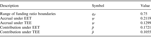
Hence, the expected equity return becomes 1.05n, while standard deviation increases by a factor of 2.24. Because the pension fund has to recover from larger shocks per period, policies are held constant over a longer range before the asymptotes of the tangent hyperbolic policy function are reached. Specifically, we set q F = 0.75. Table 4 reports the accrual and pension contribution rates for the two taxation regimes.
Table 4. Choices of pension fund parameters for the two-OLG model
6.2 Simulation results under the collective funded pension scheme
Again, the results are based on 10,000 paths of 1000 periods with the first 100 periods serving as the burn-in period. Given the pension fund's assets A t and the public debt D t, the solution to Equations (24) and (25) can be derived. This yields the individual's optimal amount of savings in period t. Again, for the TEE regime we only need to consider the setting of the pension policy instruments, because public debt is constant. Figure 8 depicts the solutions to the individual's savings problem for the policy combination α = 0.5, β = 0.5 and γ = 0.12. At this value of γ social welfare under IDC and EET is maximised. Therefore, in the sequel we will set γ = 0.12 whenever γ is held constant. The figure yields several useful insights. Panels (a) and (b) show that individuals want to increase their risk exposure by borrowing against the risk-free rate and investing the proceeds in risky assets. A reduction in the public debt lowers tax payments, while an increase in the funding ratio lowers pension contributions (panel (c)). To smooth consumption over the two periods of his life, the individual saves part of the additional resources in the first period of his life. The remaining part of these extra resources is used to increase consumption when young (panel (d)). Under EET in the absence of personal savings social welfare is CEC = 0.3346, while with personal savings it is CEC = 0.3361. The corresponding figures under TEE are CEC = 0.3285 and CEC = 0.3315, respectively. Hence, the possibility for an individual to choose his personal savings and its allocation over asset categories implies a welfare gain of <1%.
Figure 8. Personal assets, consumption and wealth when young under the EET regime (left) and TEE regime (right). The figure depicts personal assets and its components and consumption and wealth when young as a function of public debt and the funding rate when savings are optimally chosen by individuals. The instrument assumptions are α = 0.5, β = 0.5 and γ = 0.12.
Figure 9 shows welfare as measured by CEC for different adjustment policies under collective funded pension schemes. Each panel depicts a surface without and with voluntary personal savings of the individual. The former is obtained by setting Arf = Aω = 0 and obviously lies underneath the latter. We vary the pension contribution parameter α over the range 0–2.5 and the indexation policy parameter β over the range 0–1.75. For higher values of α or β, adjustments may become so large that consumption can become negative.Footnote 7 For the same reason, and in addition, we restrict ourselves to α + β ⩽ 2. Furthermore, to avoid explosive behaviour of the funding ratio for the reason explained earlier, we restrict α + β ⩾ 0.5.
Figure 9. The figure depicts certainty equivalent consumption as a function of the policy instrument parameters with and without the optimal savings decision.
The shapes of the welfare surfaces are quite similar for the two taxation regimes in panels (d) and (e). The two-OLG model implies that per period shocks are larger than under the multi-OLG setting. This has consequences for the optimal setting of the policy parameters. Hence, for given tax adjustment parameter γ social welfare reaches its maximum at lower values of α and β than before, so as to better exploit the intergenerational risk-sharing offered by the fluctuation margin in the funding ratio. Qualitatively, the results for the two-OLG model are similar without and with personal savings. They are also quite similar to the results for our multi-OLG model without personal savings. First, welfare is higher under EET than under TEE. Switching from TEE to the optimal EET regime with γ = 0.12 yields a welfare gain of roughly 1.8% with and without personal savings. The welfare gain is slightly larger in the latter case. Second, there is an internal optimum for α given (β, γ) and an internal optimum for β given (α, γ), while γ attains an internal optimum if the other two adjustment parameters are not too small. Third, both without and with personal savings contribution and indexation policies are substitutes of each other, while an increase in the tax adjustment parameter implies a decrease in the optimal contribution parameter and an increase in the contribution parameter implies an increase in the tax adjustment parameter. Except for the latter, this corresponds to the multi-OLG model.
Table 5 reports the optimal parameter combinations and welfare under the indicated policy regimes for the cases without and with personal savings. When the adjustment policies of the pension fund are selected optimally, the gains from optimal personal savings become relatively modest (between 0.4% and 1%). This may not be too surprising, because properly selected pension fund and public debt policies can go a long way in smoothing consumption. Therefore, we expect that ignoring personal savings in our multi-period OLG framework has relatively minor welfare consequences when policies are optimally selected. The locations of the optimal instrument combinations for the cases without and with personal savings are very similar under the CDC scheme. The optimal instrument combination is also quite similar with and without personal savings under a hybrid scheme when indexation is held fixed. For the remaining regimes, the most important difference concerns the indexation parameter β, which is lower when personal savings are included (as long as α + β ⩾ 0.5). When individuals have the possibility to optimally set their personal savings, the trade-off between the indexation and contribution adjustment can be shifted towards the latter, because individuals can smooth the effects of changes in their pension contributions via their personal savings.
Table 5. Performance of pension schemes under optimal parameter settings and two-OLG. Instrument parameters are set optimally for the indicated pension arrangement
7 Conclusion
This paper has studied intergenerational risk-sharing when funded pensions and public debt can be simultaneously employed for this purpose. We considered two possible instruments to stabilise pension funding ratios, namely the pension contribution and the indexation of pension rights. In addition we considered two possible tax regimes, EET and TEE. Under the former, pension contributions are paid before taxes and the pension accumulation phase is untaxed, while pension benefits are taxed. Under the TEE regime, the pension contribution is paid after taxes, while the other two phases are untaxed.
Our main results were the following. First, comparing the tax regimes, under EET participants in a pension scheme are effectively able to save a larger proportion of income for their retirement than under TEE and, therefore, benefit more from the investment returns. However, this also leads to more volatile consumption paths. From a welfare perspective, and regardless of whether we consider an individual or collective pension scheme, the former effect dominates the latter, hence EET outperforms TEE. Second, among the collective schemes, we observe that the hybrid scheme performs strictly better than both the DB scheme and the CDC scheme. By having contributions and indexation simultaneously respond to funding ratio imbalances, the volatility of consumption during working life and during retirement can be better balanced under the hybrid scheme. The social welfare gains from the hybrid scheme relative to the other, more restricted schemes can be quite large. Third, maximisation of social welfare requires setting the intensities of the different adjustment margins so as to optimally spread the adjustment burden to shocks over workers, the retired and future cohorts. As a result, contribution and indexation adjustment policies are substitutes. Hence, stronger responses of contributions to funding ratio imbalances require less active responses in indexation, and vice versa. Also, contribution and tax adjustment policies are substitutes, while indexation and tax adjustment policies are complements.
Our findings may provide some useful leads for pension system design. Generally speaking, it is beneficial to be able to deploy all risk sharing instruments considered in this paper. For example, in the Netherlands the social partners agreed that pension contributions would on average be capped at their current level, because of their financial burden on employers and employees. However, if contributions need to have a role in facilitating intergenerational risk sharing, then this is an argument for raising the retirement age, because this would allow contributions to be reduced on average and would leave more room for contributions to respond to the financial situation of the pension fund.
In future work, the analysis can be extended into a variety of directions, for example by making the labour supply decision endogenous and allowing for additional sources of risk, such as mortality, fertility and wage risks. However, the question is whether this will have consequences for the policy trade-offs that we have identified. After all, our policy adjustment parameters respond to the pension funding ratio and public debt, irrespective of the factors that cause them to move away from their targets. Finally, we have ignored demographic trends. Although beyond the scope of the present paper, including such trends would be particularly interesting, because they affect the scope for pension funds, as well as the government, to act as a shock absorber. In particular, an increase in the old-age dependency ratio reduces the base for levying pension contributions and taxes, implying potentially greater reliance on the indexation of pension entitlements as a channel for intergenerational risk sharing.
Appendix
A Derivations
A.1 Recursive liabilities
We can write the discount rate of pension entitlements recursively as
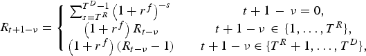 $${R_{t + 1 - \nu }} = \left\{ {\matrix{ {\sum\nolimits_{s = {T^R}}^{{T^D} - 1} {\mathop {\left( {1 + {r^f}} \right)}\nolimits^{ - s} } \,} & {\quad t + 1\, - \,\nu = 0,} \cr {\left( {1 + {r^f}} \right){R_{t - \nu }}} & {\quad t + 1 - \nu \, \in \,{\rm \{ }1, \ldots ,{T^R}{\rm \} },} \cr {\left( {1 + {r^f}} \right)\left( {{R_{t - \nu }} - 1} \right)} & {\quad t + 1 - \nu \in {\rm \{ }{T^R} + 1, \ldots ,{T^D}{\rm \} },} \cr } } \right.$$
which we can use to obtain a recursive representation for the liabilities:
$$\eqalign{{L_{t + 1}} = & \sum\limits_{\nu = t + 1 - ({T^D} - 1)}^{t + 1} \,{R_{t + 1 - \nu }}{b_{t + 1,\nu }} \cr = & \sum\limits_{\nu = t - ({T^D} - 1)}^t \,{R_{t + 1 - \nu }}{b_{t + 1,\nu }} - \underbrace {{R_{{T^D}}}{b_{t + 1,t - ({T^D} - 1)}}}_{ = 0} + \underbrace {{R_0}{b_{t + 1,t + 1}}}_{ = 0} \cr = & \sum\limits_{\nu = t - {T^D} + 1}^{t - {T^R}} \,{R_{t + 1 - \nu }}{b_{t + 1,\nu }} + \sum\limits_{\nu = t - {T^R} + 1}^t \,{R_{t + 1 - \nu }}{b_{t + 1,\nu }} \cr = & \sum\limits_{\nu = t - {T^D} + 1}^{t - {T^R}} \,(1 + {r^f})({R_{t - \nu }} - 1){b_{t + 1,\nu }} + \sum\limits_{\nu = t - {T^R} + 1}^t \,(1 + {r^f}){R_{t - \nu }}{b_{t + 1,\nu }} \cr = & \sum\limits_{\nu = t - {T^D} + 1}^{t - {T^R}} \,(1 + {r^f})({R_{t - \nu }} - 1)(1 + {I_t}){b_{t,\nu }} + \sum\limits_{\nu = t - {T^R} + 1}^t \,(1 + {r^f}){R_{t - \nu }}\left( {(1 + {I_t}){b_{t,\nu }} + \psi } \right) \cr = & (1 + {r^f})\left[ {(1 + {I_t})\sum\limits_{\nu = t - {T^D} + 1}^t \,{R_{t - \nu }}{b_{t,\nu }} - (1 + {I_t})\sum\limits_{\nu = t - {T^D} + 1}^{t - {T^R}} \,{b_{t,\nu }} + \psi \sum\limits_{\nu = t - {T^R} + 1}^t \,{R_{t - \nu }}} \right] \cr = & (1 + {r^f})\left[ {(1 + {I_t}){L_t} - {\Pi _t} + \psi \sum\limits_{t - \nu = 0}^{{T^R} - 1} \,{R_{t - \nu }}} \right].} $$A.2 Calculation of CEC
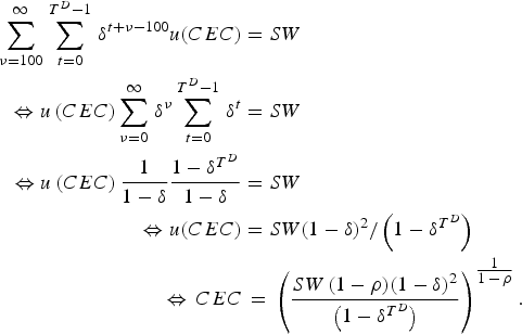 $$\eqalign{\sum\limits_{\nu = 100}^\infty \,\sum\limits_{t = 0}^{{T^D} - 1} \,{\delta ^{t + \nu - 100}}u(CEC) & = SW \cr \Leftrightarrow u\left( {CEC} \right)\sum\limits_{\nu = 0}^\infty \,{\delta ^\nu }\sum\limits_{t = 0}^{{T^D} - 1} \,{\delta ^t} & = SW \cr \Leftrightarrow u\left( {CEC} \right)\displaystyle{1 \over {1 - \delta }}\displaystyle{{1 - {\delta ^{{T^D}}}} \over {1 - \delta }} & = SW \cr \Leftrightarrow u(CEC) & = SW(1 - \delta )^2/\left( {1 - {\delta ^{{T^D}}}} \right) \cr \Leftrightarrow \,CEC & \, = \,\mathop {\left( {\displaystyle{{SW\mathop {(1 - \rho )(1 - \delta )}\nolimits^2 } \over {\left( {1 - {\delta ^{{T^D}}}} \right)}}} \right)}\nolimits^{{\textstyle{1 \over {1\, - \,\rho }}}} .} $$