2.1. Base state

We consider the Boussinesq equations for a rotating density-stratified layer of fluid inside a 3-D domain $(x,y,z)\in [0,L]\times [0,L]\times [0,H]$, with gravity and rotation along the vertical axis $z$,

(2.1)$$\begin{gather} \partial_t {\boldsymbol u} + ({\boldsymbol u}\boldsymbol{\cdot } {\boldsymbol{\nabla}}) {\boldsymbol u} + f {\boldsymbol e}_z \times {\boldsymbol u} ={-} \boldsymbol{\nabla} p + \alpha g \theta {\boldsymbol e}_z + {\nu}_{{\perp}} \Delta_{{\perp}} {\boldsymbol u}+ {\nu}_z \partial_{zz} {\boldsymbol u} , \end{gather}$$

(2.2)$$\begin{gather}\partial_t \theta + {\boldsymbol u}\boldsymbol{\cdot } {\boldsymbol{\nabla}} \theta = {\nu}_{b;\perp} \Delta_{{\perp}} \theta + {\nu}_{b;z} \partial_{zz} \theta , \end{gather}$$

where ${\boldsymbol u}(x,y,z,t)$ and $\theta (x,y,z,t)$ denote the velocity and (potential) temperature fields, $p(x,y,z,t)$ is the kinematic pressure, $\alpha$ denotes the thermal expansion coefficient, $g$ denotes gravity. The problem having very different characteristic length scales in the horizontal and vertical directions, we use two different viscosities ${\nu }_z$ and ${\nu }_{\perp }$ for the vertical and horizontal derivatives arising in the viscous term (i.e. for the $\partial _{zz}$ and $\Delta _{\perp }=\partial _{xx}+\partial _{yy}$ terms, respectively). Similarly, we use two different thermal diffusivities for horizontal (${\nu }_{b;\perp }$) and vertical (${\nu }_{b;z}$) thermal diffusion. For simplicity, temperature $\theta$ is considered to be the only stratifying agent in the equations above.

We focus on a steady base state with a vertically sheared zonal flow ${\boldsymbol u}=Sz \, {\boldsymbol e}_x$ in thermal-wind balance with a temperature gradient along the meridional direction $y$. Substitution into the equations above leads to the following base state:

(2.3a,b)\begin{equation} {\boldsymbol u}=S z {\boldsymbol e}_x , \quad \alpha g {\theta}(y,z)={-} {f S} y + N^{2} z . \end{equation}

The base state is sketched in figure 1. The meridional temperature gradient in (2.3b) is directly proportional to the vertical shear $S$ as a result of thermal wind balance, and we have included a uniform background vertical temperature gradient (uniform background buoyancy stratification $N^{2}$). In the following, we thus consider base states both with and without background vertical stratification ($N\neq 0$ and $N=0$, respectively). Strictly speaking, the base state (2.3a,b) is a solution to (2.1)–(2.2) only if supplemented with the right boundary conditions. Firstly, we neglect the tiny Ekman layer connecting the shear flow (2.3a) to the stress-free upper boundary. Secondly, a weak vertical heat flux needs to be imposed at the boundaries to maintain a base state with $N \neq 0$, the magnitude of which vanishes as the vertical diffusivities tend to zero. We validate this approach a posteriori by showing some solutions with $N = 0$. For these solutions a strong density stratification compatible with the top and bottom insulating boundary conditions emerges, and the resulting equilibrated state follows the same scaling behaviour as solutions with strong imposed background stratification $N \neq 0$. In line with the theoretical predictions to come, the emergent stratification is uniform, which justifies the compatibility between simulations performed with and without an imposed uniform background stratification $N^{2}$.

Figure 1. Base state of the Eady set-up: a plane layer of density-stratified fluid is subject to a meridional buoyancy gradient, in a frame rotating at a rate $f/2$ around the vertical axis. A uniformly sheared flow in the zonal direction $x$ coexists with the meridional buoyancy gradient as a result of thermal wind balance.

2.2. Departure from the base state: governing equations

Consider arbitrary departures from the base state,

(2.4)$$\begin{gather} {\boldsymbol u}(x,y,z,t) = {S z \, {\boldsymbol e}_x} + {\boldsymbol v} (x,y,z,t) , \end{gather}$$

(2.5)$$\begin{gather}\alpha g \theta(x,y,z,t) = {- {f S} y + N^{2} z} +b(x,y,z,t) , \end{gather}$$

where $b$ denotes the buoyancy departure. The velocity departure ${\boldsymbol v}=(u,v,w)$ is divergence-free in the Boussinesq framework, $\boldsymbol {\nabla } \boldsymbol {\cdot } {\boldsymbol v} = 0$. Substituting (2.4)–(2.5) into (2.1)–(2.2) leads to the evolution equations for ${\boldsymbol v}$ and $b$:

(2.6)$$\begin{gather} \partial_t {\boldsymbol v} + S z \partial_x {\boldsymbol v} + w S {\boldsymbol e}_x + ({\boldsymbol v} \boldsymbol{\cdot} {\boldsymbol{\nabla}}) {\boldsymbol v} + f {\boldsymbol e}_z \times {\boldsymbol v} ={-} \boldsymbol{\nabla} p + b \, {\boldsymbol e}_z + {\nu}_{{\perp}} \Delta_{{\perp}} {\boldsymbol v}+ {\nu}_z \partial_{zz} {\boldsymbol v} , \end{gather}$$

(2.7)$$\begin{gather}\partial_t b - {fS} v + N^{2} w + S z \partial_x b + {\boldsymbol v}\boldsymbol{\cdot} {\boldsymbol{\nabla}} b = {\nu}_{b;\perp} \Delta_{{\perp}} b + {\nu}_{b;z} \partial_{zz} b . \end{gather}$$

We consider periodic boundary conditions for the departure fields ${\boldsymbol v}$ and $b$ in the horizontal directions. The top and bottom boundaries are no-flux,

(2.8)\begin{equation} \partial_z b|_{z=0} = \partial_z b|_{z=H} = 0 , \end{equation}

and ${\boldsymbol v}$ satisfies free-slip boundary conditions at the top,

(2.9a,b)\begin{equation} w|_{z=H} = 0, \quad \partial_z {\boldsymbol v}_{{\perp}}|_{z=H} = 0 , \end{equation}

where ${\boldsymbol v}_{\perp }$ denotes the horizontal components of ${\boldsymbol v}$. Strictly speaking, the bottom boundary condition should be no-slip, ${\boldsymbol v}|_{z=0}={\boldsymbol 0}$. Such a no-slip boundary condition induces strong friction and pumping associated with the bottom Ekman boundary layer, of typical thickness $\sqrt {\nu _z/f}$. However, the picture of a laminar Ekman layer acting on a perfectly flat ocean bottom is probably a very naïve representation of the turbulent boundary layer near the rough ocean floor. We thus turn to a bottom boundary condition that allows us to vary the magnitude of bottom friction independently of the vertical viscosity. We replace the no-slip bottom boundary condition by the following frictional boundary condition:

(2.10a,b)\begin{equation} w|_{z=0} = 0 , \quad \partial_z {\boldsymbol v}_{{\perp}}|_{z=0} = \frac{{\kappa}H}{{\nu}_z} {\boldsymbol v}_{{\perp}}|_{z=0} . \end{equation}

This boundary condition corresponds to a linear drag law, somewhat similar to but weaker than pure Ekman friction. The strength of bottom friction can be tuned through the value of the friction coefficient $\kappa$ (not to be confused with the buoyancy diffusivities ${\nu }_{b;\perp }$ and ${\nu }_{b;z}$). As compared with a standard no-slip boundary condition, (2.10a,b) allows us to study the regime of weak bottom drag while keeping vertical viscosity values compatible with direct numerical simulation. The boundary condition (2.10a,b) reduces to a standard no-slip boundary condition for $\kappa \to \infty$, while it reduces to a stress-free boundary condition for $\kappa \to 0$. For arbitrary $\kappa$, the flow near the bottom of the fluid domain resembles a truncated Ekman spiral, with reduced shear and reduced pumping as compared with the standard Ekman boundary layer over a no-slip boundary. In Appendix A, we compute the total damping and pumping induced by the boundary condition (2.10a,b) on the bulk flow.

2.3. Non-dimensionalization

We non-dimensionalize the equations using the length scale $H$ and the time scale $f^{-1}$:

(2.11a–c)$$\begin{gather} ({x^{\sharp}},{y^{\sharp}},{z^{\sharp}})=(x,y,z) / H , \quad ({u^{\sharp}},{v^{\sharp}},{w^{\sharp}}) = (u,v,w)/(fH) , \quad {t^{\sharp}} = ft, \end{gather}$$

(2.12a–d)$$\begin{gather}{b^{\sharp}}=b/(f^{2} H) , \quad {p^{\sharp}}=p/(f^{2} H^{2}) , \quad {E}_i=\nu_i/(f H^{2}) , \quad {\kappa^{\sharp}}=\kappa/f . \end{gather}$$

Dropping the $\sharp$ symbols in the following to alleviate notations, the dimensionless governing equations are

(2.13)$$\begin{gather} \partial_t {\boldsymbol v} + Ro \, z \partial_x {\boldsymbol v} + Ro \, w {\boldsymbol e}_x + ({\boldsymbol v} \boldsymbol{\cdot} {\boldsymbol{\nabla}}) {\boldsymbol v} + {\boldsymbol e}_z \times {\boldsymbol v} ={-} \boldsymbol{\nabla} p + b \, {\boldsymbol e}_z + {{E}}_{{\perp}} \Delta_{{\perp}} {\boldsymbol v} + {{E}}_z \partial_{zz} {\boldsymbol v} , \end{gather}$$

(2.14)$$\begin{gather}\partial_t b - Ro \, v + \left(\frac{N}{f}\right)^{2} \, w + Ro \, z \partial_x b + {\boldsymbol v}\boldsymbol{\cdot } {\boldsymbol{\nabla}} b = {{E}}_{b;\perp} \Delta_{{\perp}} b + {{E}}_{b;z} \partial_{zz} b , \end{gather}$$

where the Rossby number is defined as $Ro=S/f$. The dimensionless boundary conditions are

(2.15a,b)$$\begin{gather} w|_{z=1}=0, \quad \partial_z {\boldsymbol v}_{{\perp}}|_{z=1} = 0, \end{gather}$$

(2.16a,b)$$\begin{gather}w|_{z=0}=0 , \quad \partial_z {\boldsymbol v}_{{\perp}}|_{z=0} = \frac{{\kappa}}{{{E}}_z} {\boldsymbol v}_{{\perp}}|_{z=0} , \end{gather}$$

(2.17)$$\begin{gather}\partial_z b|_{z=0} = \partial_z b|_{z=1} = 0 . \end{gather}$$

2.4. Numerical implementation

We wish to characterize the buoyancy transport achieved by statistically steady solutions to (2.13)–(2.14) with the boundary conditions (2.15a,b) through (2.17) (see Bachman & Fox-Kemper (Reference Bachman and Fox-Kemper2013) for a study of the spin-down problem). Denoting as $\left \langle\, \cdot\, \right \rangle$ a time and volume average, we will consider the time- and volume-averaged meridional and vertical buoyancy fluxes, $\left \langle vb \right \rangle$ and $\left \langle wb \right \rangle$, respectively. We also consider the vertical profiles of the meridional and vertical buoyancy fluxes, $\overline {vb}(z)$ and $\overline {wb}(z)$, where the overbar denotes a horizontal area average together with a time average. Finally, a quantity of interest is the emergent stratification $\bar {b}(z)$ that arises in the equilibrated state. The total vertical buoyancy stratification is $(N/f)^{2} z+\bar {b}(z)$, and, assuming that the emergent stratification is approximately uniform, we define the Rossby deformation radius $\lambda$ as

(2.18)\begin{equation} \lambda=\sqrt{\left(\frac{N}{f}\right)^{2}+\bar{b}(1)-\bar{b}(0)} , \end{equation}

where $\lambda$ is non-dimensionalized with $H$.

We have performed a suite of numerical simulations of (2.13)–(2.14) using Coral, a pseudospectral, scalable, time-stepping solver for differential equations (Miquel Reference Miquel2021). In Coral, the top and bottom boundary conditions are imposed through basis recombination. The variables are expanded on bases of functions obtained as tensor products of Fourier modes along the horizontal and suitable linear combinations of Chebyshev polynomials, each of which obeys the boundary conditions along $z$. The divergence-free constraint is readily implemented in Coral by introducing the standard toroidal and poloidal velocity potentials $\psi (x,y,z)$ and $\phi (x,y,z)$, respectively. The frictional bottom boundary condition is dealt with by defining modified velocity potentials $\tilde {\psi }$ and $\tilde {\phi }$ as $\psi (x,y,z) = P_\psi (z) \tilde {\psi }(x,y,z)$ and $\phi (x,y,z) = P_\phi (z) \tilde {\phi }(x,y,z)$, where $P_\psi (z)$ and $P_\phi (z)$ are carefully chosen quadratic polynomials, the coefficients of which depend on the drag coefficient. In particular, these polynomials are tailored so that imposing the Robin boundary conditions (2.16a,b) on the velocity field amounts to imposing standard stress-free type boundary conditions for the modified potentials: $\partial _z \tilde {\psi } =\tilde {\phi } = \partial _{zz}\tilde {\phi }=0$. We can thus solve for $\tilde {\psi }$ and $\tilde {\phi }$ using standard Galerkin basis recombination. The code has been benchmarked by careful comparison with results from linear stability analysis; checks that the various power integrals are exactly satisfied in the nonlinear regime, and comparison of the overall buoyancy transport with a run of the same problem performed with the Dedalus solver (Burns et al. Reference Burns, Vasil, Oishi, Lecoanet and Brown2020) have also been done. The numerical runs are initialized with either low-amplitude noise or a checkpoint from a previous simulation. We average the relevant quantities over the statistically steady regime, and make sure that the statistics are correctly converged by comparing with averages performed over the first half of the statistically steady signal only.

3.1. The low-diffusivity regime

We focus on the regime where the horizontal extent of the domain is large compared with the energy-containing scale and the mixing length of the flow (estimated as the ratio of root mean square horizontal buoyancy fluctuations divided by the meridional buoyancy gradient, see e.g. Thompson & Young (Reference Thompson and Young2006)). Through variations of the domain size, we checked that the transport properties of the flow are then independent of the horizontal domain size (for brevity, we do not report these validation runs in the tables below). The diffusivities are chosen to be equal for momentum and buoyancy, i.e. ${{E}}_{b;\perp }={{E}}_{\perp }$ and ${{E}}_{b;z}={{E}}_{z}$ in all of the numerical runs. This corresponds to setting the Prandtl number to unity, an appropriate choice in the present context where the viscosities and diffusivities represent mixing by small-scale turbulence, and not molecular processes. The horizontal diffusivities are small enough not to affect the transport properties of the equilibrated flow. The role of the vertical diffusivities is more subtle: anticipating the results in §§ 3 and 4, we choose small enough vertical diffusivities for the transport properties of the flow to be well-described by bulk diffusivity-free QG dynamics with bottom friction. In that regime, however, the emergent stratification depends on the vertical buoyancy diffusivity, as described in § 4.2. Table 1 lists the various control parameters for the numerical runs considered in the present study: we vary the background stratification, the Rossby number, the diffusivities and the friction coefficient.

Table 1. Control and emergent parameter values for the runs retained in the main study. For all the runs $E_{b;z}=E_z$ and $E_{b;\perp }=E_{\perp }$. The last column indicates the number of modes in each direction used for the numerical simulation.

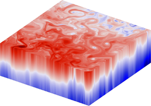
The qualitative aspect of the equilibrated flow is illustrated in figure 2, where we show a 3-D rendering of the total buoyancy field together with horizontal slices of the dimensionless vertical vorticity $\zeta$ at mid-depth and at the top surface. We observe that the flow remains strongly stratified in the equilibrated state, with weak isopycnal slopes in the bulk of the fluid domain. Figure 2(a–c) correspond to a run that is marginally QG and has very low dimensionless drag. The bulk vertical vorticity exhibits a relatively dilute gas of vortices, although there is some asymmetry between cyclones and anticyclones. This asymmetry probably stems from the sharp non-QG frontal structures that develop at the surface (Hoskins & Bretherton Reference Hoskins and Bretherton1971; Klein et al. Reference Klein, Hua, Lapeyre, Capet, Le Gentil and Sasaki2008; Ragone & Badin Reference Ragone and Badin2016; Siegelman et al. Reference Siegelman, Klein, Rivière, Thompson, Torres, Flexas and Menemenlis2020), see figure 2(c). We will see in the following that the transport properties of this flow are correctly described by QG theory despite the slight cyclone/anticyclone asymmetry of the interior flow. Figure 2(d,e) illustrate a run in the strongly QG regime with moderately low drag. The vortex gas is less dilute as a result of the larger drag. The QG cyclone–anticyclone symmetry is well-satisfied both at mid-depth (figure 2d) and in the surface quasigeostrophic (SQG) fronts visible in figure 2(e).

Figure 2. Equilibrated baroclinic turbulence illustrated with snapshots from (a–c) run 21 (low drag) and (d,e run 3 (moderate drag). (a) A 3-D rendering of the total buoyancy field. Notice the very different vertical and horizontal scales, and thus the very weak isopycnal slopes. (b) The vertical vorticity at mid-depth shows coherent vortices, with slight cyclone/anticyclone asymmetry in this marginally QG run. (c) The surface vertical vorticity exhibits sharp frontal structures where relative vorticity greatly exceeds planetary vorticity. Panels (d,e) are the same as panels (b,c), but for larger dimensionless drag $\kappa _*$ in a strongly QG regime. The vorticity at mid-depth shows a less dilute vortex gas than in panel (b). The QG cyclone/anticyclone symmetry is well satisfied, including in the sharp surface QG (SQG) frontal structures visible in panel (e).

In figure 3, we show the overall meridional buoyancy flux $\left \langle vb \right \rangle$ as a function of the friction coefficient $\kappa$. The buoyancy flux varies over more than four orders of magnitude over the entire data set. Meridional transport increases as the friction coefficient decreases (for otherwise constant parameters), and it decreases rapidly with decreasing Rossby number.

Figure 3. Raw meridional buoyancy flux as a function of the friction coefficient for the 22 numerical runs. The symbols correspond to different values of the Rossby number, while colour codes correspond to the background stratification. The meridional flux increases with decreasing friction coefficient for otherwise constant parameters.

3.2. Bulk QG dynamics: further reducing the number of control parameters

The qualitative features of the equilibrated flows in figure 2 point to QG dynamics. One can derive the QG approximation to the Boussinesq Eady system following the standard procedure reviewed in Appendix B (see also Salmon Reference Salmon1998; Vallis Reference Vallis2006). Decompose the pressure field into a time and horizontal mean $\bar {p}(z)$ plus fluctuations $\tilde {p}(x,y,z,t)$:

(3.1)\begin{equation} {p}(x,y,z,t)=\bar{p}(z)+\tilde{p}(x,y,z,t), \quad \text{with} \ \bar{\tilde{p}}=0 . \end{equation}

Notice that the horizontal and time derivatives of $p$ and $\tilde {p}$ are equal, so that $p$ and $\tilde {p}$ can be used interchangeably in many (but not all) of the expressions to come. Assuming that the emergent stratification is approximately uniform and neglecting the diffusive terms in the bulk of the flow, the PV conservation equation reads (see Appendix B)

(3.2)\begin{equation} \partial_t q + J(\tilde{p},q) + Ro \, z \, \partial_x q = 0 , \end{equation}

where the PV is

(3.3)\begin{equation} q = {\nabla}_{{\perp}}^{2} \tilde{p} + \frac{\partial_{zz} \tilde{p}}{\lambda^{2}} . \end{equation}

The boundary conditions are the buoyancy equation written at the boundaries, remembering the hydrostatic relation ${b}=\partial _z {p}$. At the top free-surface one obtains

(3.4)\begin{equation} \partial_{tz} \tilde{p}|_1 - Ro \, \partial_x \tilde{p}|_1 + Ro \, \partial_{xz} \tilde{p}|_1 + J(\tilde{p}|_1,\partial_z \tilde{p}|_1) = 0 . \end{equation}

The second boundary condition stems from the buoyancy equation written just above the partial Ekman layer connecting the bulk flow to the frictional bottom boundary condition (a height denoted as $z=0^{+}$),

(3.5)\begin{equation} \partial_{tz} \tilde{p}|_{0^{+}} - Ro \, \partial_x \tilde{p}|_{0^{+}} + J(\tilde{p}|_{0^{+}},\partial_z \tilde{p}|_{0^{+}}) + \lambda^{2} w|_{0^{+}} = 0 , \end{equation}

where $w|_{0^{+}}$ denotes the vertical pumping velocity induced by the partial Ekman layer. As shown in Appendix A, this pumping velocity takes the form

(3.6)\begin{equation} w|_{0^{+}} = \kappa_{eff} \zeta|_{0^{+}} =\kappa_{eff} \Delta_{{\perp}} \tilde{p}|_{0^{+}} , \end{equation}

where the effective friction coefficient acting on the interior flow is

(3.7)\begin{equation} \kappa_{eff} = \dfrac{\sqrt{2 {E}_z}}{1+ \dfrac{\sqrt{2 {E}_z}}{\kappa}+\dfrac{{E}_z}{\kappa^{2}}} \times \left(\dfrac{1}{2}+ \sqrt{\dfrac{{E}_z}{2}} \dfrac{1}{\kappa} \right) , \end{equation}

both $\kappa$ and $\kappa _{eff}$ being non-dimensionalized with $f$. Expression (3.7) reduces to the standard Ekman friction coefficient in the no-slip limit $\kappa \to \infty$ (Pedlosky Reference Pedlosky1979). The buoyancy equation at $z=0^{+}$ finally reads

(3.8)\begin{equation} \partial_{tz} \tilde{p}|_{0^{+}} - Ro \, \partial_x \tilde{p}|_{0^{+}} + J(\tilde{p}|_{0^{+}},\partial_z \tilde{p}|_{0^{+}}) + \lambda^{2} \kappa_{eff} \Delta_{{\perp}} \tilde{p}|_{0^{+}}= 0 . \end{equation}

The QG dynamics is governed by the conservation equation (3.2) for the bulk PV (3.3), with the top and bottom boundary conditions (3.4) and (3.8). The fluid communicates in the vertical direction through slight vertical displacements of the isopycnals, which induce modifications in vertical vorticity $\zeta =\Delta _{\perp } p$ through the conservation of PV (for the specific case of a cylindrical fluid column contained between two isopycnals, this process can be understood as the conservation of angular momentum as the column gets compressed or stretched). Diffusion plays no role in this process, the consequence being that $\kappa$ and ${E}_z$ enter the QG dynamics only through the effective friction coefficient $\kappa _{eff}$ associated with pumping in the bottom (partial) Ekman layer. The number of dimensionless parameters relevant to the QG regime can be further reduced through the introduction of the QG scalings,

(3.9a–e)\begin{equation} t= \frac{\lambda}{Ro} T , \quad x= \lambda X, \quad y= \lambda Y , \quad \tilde{p}=Ro \lambda \, P(X,Y,z,T) , \quad q = \frac{Ro}{\lambda} Q(X,Y,z,T) . \end{equation}

Through this change of variables the QG equations become

(3.10)$$\begin{gather} \partial_T Q + J_{\boldsymbol X}(P,Q)+z \partial_X Q = 0 , \end{gather}$$

(3.11)$$\begin{gather}Q = \Delta_{{\boldsymbol X},\perp} P + \partial_{zz}P , \end{gather}$$

(3.12)$$\begin{gather}\partial_{Tz} P|_1 - \partial_X P|_1 + \partial_{Xz} P|_1 + J_{\boldsymbol X}(P|_1,\partial_z P|_1) = 0 , \end{gather}$$

(3.13)$$\begin{gather}\partial_{Tz} P|_{0^{+}} - \partial_X P|_{0^{+}} + J_{\boldsymbol X}(P|_{0^{+}},\partial_z P|_{0^{+}}) + \frac{\kappa_{eff} \lambda}{Ro} \Delta_{{\boldsymbol X},\perp} P|_{0^{+}} = 0 , \end{gather}$$

where $J_{\boldsymbol X}(f,g)=\partial _X f \partial _Y g-\partial _Y f \partial _X g$ and $\Delta _{{\boldsymbol X},\perp } = \partial _{XX}+ \partial _{YY}$. An instructive feature of this set of equations is that it involves a single control parameter,

(3.14)\begin{equation} \kappa_*= \frac{\kappa_{eff} \lambda}{Ro} , \end{equation}

which is the Boussinesq equivalent of the relevant dimensionless drag coefficient in the QG framework (Thompson & Young Reference Thompson and Young2006; Gallet & Ferrari Reference Gallet and Ferrari2020). The equilibrated solutions to the set of equations (3.10)–(3.13) are characterized by a meridional buoyancy transport $D_*=\left \langle \partial _X P \partial _z P \right \rangle =\left \langle v b \right \rangle /(Ro^{2} \lambda )$ that depends only on $\kappa _*$. We conclude that

(3.15)\begin{equation} D_* \equiv \frac{\left\langle v b \right\rangle}{Ro^{2} \lambda}= {\mathcal{F}} \left( \kappa_* = \frac{\kappa_{eff} \lambda}{Ro} \right) , \end{equation}

where the unknown function ${\mathcal {F}}$ denotes the dependence of the QG buoyancy eddy diffusivity $D_*$ on the QG dimensionless drag $\kappa _*$. As discussed in Thompson & Young (Reference Thompson and Young2006) and Gallet & Ferrari (Reference Gallet and Ferrari2020), the 2LQG equivalent of $D_*$ readily quantifies the ratio of the meridional buoyancy flux over the meridional buoyancy gradient, hence the name ‘diffusivity’. Indeed, while the change of variables above provides a rigorous way to identify $D_*$ and $\kappa _*$ as the ‘order’ and ‘control’ parameters of the QG regime, the form of $D_*$ and $\kappa _*$ could have been guessed from studies of the strongly idealized 2LQG model: as shown in Thompson & Young (Reference Thompson and Young2006), the 2LQG model on the $f$-plane reduces to the study of $D_*$ versus $\kappa _*$, where $D_*$ is the meridional flux divided by the product of the deformation radius with the squared shearing velocity, while $\kappa _*$ is the bottom drag coefficient multiplied by the deformation radius and divided by the shearing velocity.

Equation (3.15) suggests a quantitative way to assess whether meridional buoyancy transport is governed by QG dynamics in the present simulations of the Boussinesq system: in figure 4, we plot $D_*$ as a function of $\kappa _*$ for the entire dataset. This representation leads to a collapse onto a master curve of the entire data set, which includes various values of the Rossby number, background stratification and vertical Ekman numbers. This confirms the validity of the QG scalings for bulk transport in the present numerical data, despite the emergence of potentially non-QG frontal dynamics near the boundaries.

Figure 4. Dimensionless eddy-induced diffusivity as a function of the dimensionless effective friction coefficient, using the QG non-dimensionalization. The entire data set falls onto a master curve, indicating that QG dynamics governs the overall buoyancy transport. Same symbols and colours as in figure 3. The thick vertical dashed lines indicate the predicted values of $\kappa _*$ according to (4.9) for the runs without background stratification (black circles). The predicted values of $\kappa _*$ agree with the direct numerical simulation ones within $5\,\%$. Black crosses are the solutions to the QG system. The solid line is the vortex-gas prediction (3.16) with $c_1=0.32$ and $c_2=0.61$.

We further compare the results of the Boussinesq system with QG theory by solving the QG Eady problem explicitly. A trivial solution to the QG PV conservation equation (3.10) is $Q=0$. In Appendix B, we recall how this constraint leads to an inversion relation providing $P|_{1}$ and $P|_{0^{+}}$ in terms of $\partial _z P|_{1}$ and $\partial _z P|_{0^{+}}$ at each time step. Solving the 3-D QG problem then reduces to solving the coupled equations (3.12) and (3.13) for the two-dimensional (2-D) fields $\partial _z P|_{1}$ and $\partial _z P|_{0^{+}}$, using the inversion relation to infer $P|_{1}$ and $P|_{0^{+}}$ at each time step. The approach is very similar to SQG (Blumen Reference Blumen1978; Held et al. Reference Held, Pierrehumbert, Garner and Swanson1995; Callies et al. Reference Callies, Flierl, Ferrari and Fox-Kemper2016; Lapeyre Reference Lapeyre2017), the difference being that there are two horizontal boundaries in the present system (at top and bottom), as opposed to a single horizontal boundary in the standard SQG system. The second boundary crucially allows for the emergence of depth-invariant barotropic eddies in the present system. The effectively 2-D equations are solved on a graphics processing unit in a large enough domain for finite-size effects to be negligible. To damp the small-scale filaments, we also add hyperviscous terms $-\mu \Delta _{{\boldsymbol X},\perp }^{4} \partial _{z} P|_1$ and $-\mu \Delta _{{\boldsymbol X},\perp }^{4} \partial _{z} P|_{0^{+}}$ to the right-hand sides of (3.12) and (3.13), respectively, where the dimensionless hyperdiffusivity $\mu$ is chosen small enough to not affect the meridional heat flux in the equilibrated state. The resulting data points are plotted using crosses in figure 4. They agree very well with the 3-D Boussinesq data, indicating that PV vanishes in the interior of the 3-D domain as a result of the dissipative terms, with negligible PV injection by frontal structures at the boundaries (in contrast with zonally invariant 2-D primitive-equation models, see Nakamura & Held (Reference Nakamura and Held1989) and Garner, Nakamura & Held (Reference Garner, Nakamura and Held1992)).

To summarize, we have established that meridional transport in the equilibrated Boussinesq Eady system is governed by QG dynamics, as illustrated by the collapse of the Boussinesq data in the representation of figure 4 and their good agreement with solutions of the QG system. Developing a theory for the magnitude of the meridional transport in the equilibrated Eady problem then reduces to the determination of the function ${\mathcal {F}}$ in the scaling relation (3.15).

3.3. Vortex-gas scaling theory

We recently introduced such a scaling theory, coined the vortex-gas scaling regime (Gallet & Ferrari Reference Gallet and Ferrari2020), within the framework of the 2LQG model. The central idea is that the barotropic flow consists of a dilute gas of isolated vortices wandering around through mutual advection (Carnevale et al. Reference Carnevale, McWilliams, Pomeau, Weiss and Young1991; Thompson & Young Reference Thompson and Young2006). The vortex cores are small compared with the intervortex distance, with a radius comparable to the Rossby deformation radius. Buoyancy fluctuations arise through the distortion of the background meridional gradient by the vortical flow. Focussing on a single barotropic vortex dipole shows that the mixing length is comparable to the intervortex distance, while the diffusivity is given by the product of the intervortex distance with the velocity at which the vortex cores move. Two energetic arguments complete the scaling theory. First, a typical velocity scale is estimated by equating the potential energy drop with the final kinetic energy as a fluid column travels over one mixing length (seen as the mean-free path of the turbulent fluid motion). This ‘slantwise free-fall’ argument yields the typical velocity of a fluid column located between two vortices, which is also the velocity scale at which the vortex cores move. Second, at equilibrium the energy released through baroclinic instability must be balanced by frictional dissipation. Significantly larger velocities arise at the immediate periphery of the vortex cores, where fluid particles circle rapidly without transporting much buoyancy. These large velocities are associated with large frictional dissipation, with important consequences for the energy power integral, which is the last scaling relation of the theory. This line of arguments provides a theoretical expression for the function ${\mathcal {F}}$ in (3.15). Specifically, for linear bottom friction we obtain

(3.16)\begin{equation} D_* = c_1 \exp \left({\frac{c_2}{\kappa_*}}\right) , \end{equation}

where $c_1$ and $c_2$ are adjustable parameters that may depend on details of the specific model. Based on low-drag simulations of the 2LQG model with equal layer depths, we estimated $c_1^{(2LQG)}\simeq 2.0$ and $c_2^{(2LQG)}\simeq 0.72$ (Gallet & Ferrari Reference Gallet and Ferrari2021). For the present Boussinesq Eady data, we show in figure 4 that the vortex-gas prediction (3.16) accurately captures the master curve, with $c_1=0.32$ and $c_2=0.61$. This indicates that the physical intuition gathered from the 2LQG model carries over to the fully 3-D Eady model.

4.1. Bulk eddy transport is along isopycnals

In a similar fashion to (3.1), decompose the buoyancy field into a time and horizontal mean $\bar {b}(z)$ plus fluctuations $\tilde {b}(x,y,z,t)$:

(4.1)\begin{equation} {b}(x,y,z,t)=\bar{b}(z)+\tilde{b}(x,y,z,t), \quad \text{with} \ \bar{\tilde{b}}=0 . \end{equation}

Upon multiplying the buoyancy equation (2.14) with $b$ before averaging temporally and horizontally, assuming that the fluctuations are much weaker than the mean, $\tilde {b} \ll \bar {b}$, one obtains

(4.2)\begin{equation} -Ro \, \overline{vb} + \left[ \left( \frac{N}{f}\right)^{2} + \partial_z \bar{b} \right] \overline{wb} \simeq{-}{{E}}_{b;\perp} \overline{|\boldsymbol{\nabla}_{{\perp}} b|^{2}} + {{E}}_{b;z} \overline{b \partial_{zz}b} . \end{equation}

If the diffusive terms on the right-hand side are negligible, we recover the standard conclusion that the eddy-induced buoyancy current is along isopycnals (Gent & Mcwilliams Reference Gent and Mcwilliams1990; Young Reference Young2012). In terms of the overall magnitude of the vertical buoyancy flux, this leads to the simple relation,

(4.3)\begin{equation} \left\langle wb \right\rangle \simeq \frac{Ro}{\lambda^{2}} \left\langle vb \right\rangle , \end{equation}

the slope of the isopycnals being $Ro/\lambda ^{2}$. In figure 5 we plot the ratio of the left-hand side over the right-hand side of (4.3), denoted as ${r}$, for solutions of the Boussinesq system. This ratio is indeed approximately constant at low drag, with a value ${r} \simeq 0.85$ close to unity, the slight departure from one being due to the small diffusive contributions in (4.2). The ratio ${r}$ approaches unity if the diffusive terms are small enough in a regime where the assumptions of QG are well satisfied. Solutions to the QG system – (3.12)–(3.13) together with inversion relations (B17)–(B18) – satisfy ${r}=1$ exactly. Overall, the combination of the vortex-gas scaling prediction with the Gent–McWilliams argument leads to a good theoretical prediction for the vertical buoyancy flux,

(4.4)\begin{equation} \left\langle wb \right\rangle = c_1 {r} \frac{Ro^{3}}{\lambda} \exp \left({\frac{c_2}{\kappa_*}}\right) \simeq c_1 \frac{Ro^{3}}{\lambda} \exp \left({\frac{c_2}{\kappa_*}}\right) , \end{equation}

as illustrated in figure 5.

Figure 5. Inset: ratio ${r}$ between the two sides of the approximate relation (4.3). This ratio is always close to unity, with a typical value ${r}\simeq 0.85$ over the entire data set. This ratio approaches unity as the diffusivities are lowered, indicating along-isopycnal transport. Main figure: dimensionless vertical buoyancy flux as a function of the dimensionless effective friction coefficient, both being non-dimensionalized following the QG scalings. Combining the vortex-gas theory with pure along-isopycnal transport leads to the prediction on the right-hand side of (4.4), shown as a solid line. Same symbols and colours as in figure 3.

4.2. Strength of the emergent stratification

One then estimates the emergent stratification from the vertical buoyancy flux through the potential energy evolution equation. Multiplying the buoyancy equation (2.14) by $z$ before averaging over space and time yields, after using $\bar {w}=0$ and performing some integrations by parts using the boundary conditions,

(4.5)\begin{equation} Ro \int_0^{1} z \bar{v} \, \mathrm{d}z + \left\langle wb \right\rangle = {E}_{b; z} \left[ \bar{b}(1)-\bar{b}(0) \right] . \end{equation}

We wish to show that the term involving the mean meridional flow $\bar {v}(z)$ is negligible as compared with the vertical buoyancy flux on the left-hand side. This mean meridional velocity corresponds to an ageostrophic flow, because a mean zonal buoyancy gradient maintaining $\bar {v}(z)$ through thermal wind balance would be incompatible with the periodic boundary conditions. The profile $\bar {v}(z)$ can be estimated by time- and area-averaging the zonal component of the momentum equation (2.6),

(4.6)\begin{equation} \bar{v} = \partial_z \overline{wu} - E_z \partial_{zz} \bar{u} . \end{equation}

The second term on the right-hand side is negligible in the bulk of the domain because $E_z \ll 1$. The first term on the right-hand side involves $\overline {wu}$. It leads to a contribution $-Ro \left \langle wu \right \rangle$ to the left-hand side of (4.5), to be compared with the second term, $\left \langle wb \right \rangle$. A crude estimate of the ratio of these two contributions is $Ro { \left \langle u^{2} \right \rangle ^{1/2}}/{\left \langle b^{2} \right \rangle ^{1/2}}$, which using thermal-wind balance for a flow of horizontal scale $\lambda$ is of order $Ro /\lambda \ll 1$. This simple estimate is a first indication that the $\bar {v}$ term in (4.5) is negligible as compared with the vertical buoyancy flux.

We stress the fact, however, that $\left \langle wu \right \rangle$ and $\bar {v}$ are even smaller than the crude estimate above. Indeed, to lowest order the magnitude of $\left \langle wu \right \rangle$ can be estimated using QG theory, the diagnostic vertical velocity being inferred from (B7). One can then leverage the cyclone–anticyclone symmetry of the QG system to show that the resulting $\overline {wu}$ vanishes, as explained in Appendix B.3. In other words, while QG dynamics induces a non-zero vertical buoyancy flux $\overline {wb}$ in the bulk of the domain, it leads to a vanishing vertical flux of zonal momentum $\overline {wu}$ for symmetry reasons. Non-zero $\overline {wu}$ in the bulk may only arise at next order in the QG expansion, where cyclone–anticyclone symmetry is broken (Muraki, Snyder & Rotunno Reference Muraki, Snyder and Rotunno1999; Hakim, Snyder & Muraki Reference Hakim, Snyder and Muraki2002; Gallet et al. Reference Gallet, Campagne, Cortet and Moisy2014). We conclude that $\left \langle wu \right \rangle$ is smaller than the estimate of the previous paragraph by (at least) a factor corresponding to the isopycnal slope, $Ro/\lambda ^{2} \ll 1$. The $\bar {v}$ term is thus fully negligible as compared with $\left \langle wb \right \rangle$ in (4.5).

Having shown that the dominant balance in (4.5) is between the vertical buoyancy flux and the diffusive flux associated with the emergent stratification, we obtain the following expression for the emergent stratification:

(4.7)\begin{equation} \bar{b}(1)-\bar{b}(0) \simeq \frac{\left\langle wb \right\rangle}{{E}_{b; z}} . \end{equation}

One should notice that the vertical buoyancy diffusivity comes back into play through the coefficient ${E}_{b; z}$ in the denominator. While the vertical momentum diffusivity (the viscosity coefficient) affects the scaling behaviour of the system only marginally, through a modification of the effective friction coefficient (3.7), the vertical buoyancy diffusivity greatly impacts the emergent stratification (4.7). The transport properties of the system are independent of the vertical buoyancy diffusivity only in the regime where the emergent stratification (4.7) is negligible as compared with the imposed background stratification. Otherwise, changes in ${E}_{b; z}$ induce changes in the emergent stratification (4.7) and thus in the Rossby deformation radius $\lambda$, the consequence being that the transport properties of the equilibrated state are shifted following the QG master curves in figures 4 and 5. From (4.7), we can estimate the emergent stratification directly in terms of the control parameters of the problem. While this can be done for an arbitrary background stratification, we focus on two limiting situations: the case without imposed background stratification; and the case where the emergent stratification is negligible as compared with the imposed background one.

In the absence of imposed background stratification, where $\bar {b}(1)-\bar {b}(0)=\lambda ^{2}$, we insert expression (4.4) for the vertical flux into (4.7), before writing the resulting relation as

(4.8)\begin{equation} \left(\frac{c_2}{\kappa_*} \right)^{3} \,{\rm e}^{{c_2}/{\kappa_*}} = \frac{c_2^{3}}{c_1} \times \frac{{E}_{b; z} }{\kappa_{eff}^{3}} . \end{equation}

We invert this relation to obtain ${c_2}/{\kappa _*}$, which leads to the following expression for the emergent Rossby deformation radius (emergent stratification):

(4.9)\begin{equation} \lambda = \dfrac{c_2 Ro}{3 \kappa_{eff} {\mathcal{W}}\left[ \dfrac{c_2 }{3 c_1^{1/3}} \times \dfrac{ {E}_{b; z}^{1/3}}{\kappa_{eff}} \right]},\quad \text{that is}\ \kappa_* = \dfrac{c_2}{3 {\mathcal{W}}\left[ \dfrac{c_2 }{3 c_1^{1/3}} \times \dfrac{ {E}_{b; z}^{1/3}}{\kappa_{eff}} \right]} , \end{equation}

where ${\mathcal {W}}$ denotes the Lambert function. These equations relate emergent quantities (on the left-hand side) to control parameters only (on the right-hand side). The first expression in (4.9) provides the emergent stratification, while the second one readily gives the dimensionless friction $\kappa _*$ arising in the QG framework (the abscissa in figures 4 and 5). We have performed two numerical runs without background stratification to validate these predictions. In figure 4, we show that the resulting meridional flux falls onto the master curve, at an abscissa given by the theoretical expression (4.9) within $5\,\%$ accuracy.

We now consider the case of a non-zero imposed background stratification $(N/f)^{2}$. We wish to determine when the emergent stratification is negligible as compared with the imposed one. To wit, we estimate the emergent stratification by inserting into (4.7) expression (4.4) for the vertical flux, in which we replace $\lambda$ with $N/f$. Demanding that this emergent stratification be negligible as compared with the imposed one, $(N/f)^{2}$, then amounts to satisfying the inequality,

(4.10)\begin{equation} {E}_{b; z} \gg c_1 \frac{Ro^{3}}{(N/f)^{3}} \exp \left( \frac{c_2 Ro}{\kappa_{eff} N/f} \right) . \end{equation}

The criterion (4.10) is expressed in terms of the control parameters of the system only. It allows one to assess a priori whether or not the emergent stratification is negligible as compared with the background one, as illustrated in figure 6. When the inequality (4.10) is satisfied, the emergent stratification is negligible and the meridional and vertical buoyancy fluxes are readily obtained by replacing $\lambda$ with $(N/f)$ in expressions (3.16) and (4.4).

Figure 6. Ratio of the emergent stratification, $\bar {b}(1)-\bar {b}(0)$, over the background one, $(N/f)^{2}$, versus the ratio of the right-hand side of (4.10) over $E_{b;z}$. In agreement with the criterion (4.10), the emergent stratification is negligible as compared with the background one when the abscissa is much less than unity. In this regime the abscissa readily provides the theoretical prediction for the emergent stratification divided by the background one, and indeed the data points fall onto the diagonal. The emergent stratification becomes comparable to the background one as the abscissa approaches unity. Same symbols and colours as in figure 3.

To summarize, combining the vortex-gas scaling theory with both the along-isopycnal- transport argument and a simple advective–diffusive buoyancy-flux balance along the vertical direction, we obtain theoretical expressions for the meridional buoyancy flux, the vertical buoyancy flux and the emergent stratification in terms of the control parameters of the problem.

5.1. Depth-invariant meridional flux

The QG framework readily provides a prediction for the vertical structure of the meridional buoyancy flux. According to (3.2), the PV (3.3) is a material invariant of the undamped system. If the initial condition corresponds to vanishing PV, the PV will remain zero at subsequent times and the meridional PV flux vanishes at any depth. Within the QG framework this PV flux reads (Vallis Reference Vallis2006)

(5.1)\begin{equation} 0 = \overline{vq} = \overline{p_x p_{xx}} + \overline{p_x p_{yy}} + \frac{1}{\lambda^{2}} \overline{p_x p_{zz}} = \frac{1}{\lambda^{2}} \partial_z (\overline{p_x p_z}) = \frac{1}{\lambda^{2}} \partial_z \overline{vb}, \end{equation}

which indicates that the meridional buoyancy flux is depth-independent. This QG prediction turns out to be in very good agreement with the numerical data, as illustrated by the meridional buoyancy flux profiles in figure 7: the low-drag profile in figure 7(a) is depth-independent to very good accuracy. The moderate-drag profile in figure 7(c) is also depth-independent in the interior, with slight departures restricted to a boundary-layer near the surface. Finally, solutions to the QG system – (3.12)–(3.13) together with inversion relations (B17)–(B18) – are characterized by depth-independent meridional flux profiles by construction.

Figure 7. (a–d) Profiles of the scaled meridional and vertical buoyancy fluxes arising in (4.2), and profiles of horizontal TKE, for (a,b) run 21 ($\kappa _*=0.139$) and (c,d) run3 ($\kappa _*=0.595$). For both runs the meridional flux is approximately depth-independent, in agreement with the QG prediction. Panels (a,b) correspond to the low-drag regime, with moderately low Ekman numbers. The vertical flux retains some depth-dependence near the boundaries. By contrast, for the very low-diffusivity run of the panels (c,d) the vertical buoyancy flux is approximately depth-invariant. The TKE profiles show the gradual barotropization of the flow as we go from (c,d) moderately low drag to (a,b) very low drag. (e) The diapycnal mixing associated with the diffusive terms in (4.2) decreases as the diffusivities are lowered. Here both the vertical and horizontal diffusivities are simultaneously decreased by factors of 2 and factors of 4, the lowest values (thick black curve) corresponding to run 3 (c,d).

5.2. Vertical flux and bulk stratification

Having determined the vertical structure of the meridional buoyancy flux, we turn to the vertical buoyancy flux using relation (4.2). We have seen that the overall contribution from dissipative terms on the right-hand side of that relation is sometimes not entirely negligible, with ${r} \simeq 0.85$ instead of ${r}=1$, but how is that contribution distributed with depth?

We answer that question in figure 7, where we compare the two flux terms on the left-hand side of (4.2). Within the central half of the domain, these two terms balance each other to a good accuracy: the eddy transport current is directed along isopycnals in the bulk of the domain. However, for several runs this balance becomes unsatisfactory as we move closer to the top and bottom boundaries, where the vertical flux needs to be compatible with the boundary conditions: $w$ vanishes at the top free surface, while it matches the pumping velocity near the bottom boundary. In other words, the diffusive terms in (4.2) are not entirely negligible near the boundaries. In particular, we expect a strong contribution from the horizontal diffusive term in (4.2) at the surface, where SQG dynamics predicts a forward cascade of buoyancy (towards small horizontal scales) (Held et al. Reference Held, Pierrehumbert, Garner and Swanson1995; Lapeyre Reference Lapeyre2017). The depth-independent meridional buoyancy flux in (4.2) is thus balanced by the vertical buoyancy flux term in the bulk of the domain and by the diffusive terms at the boundaries. The thickness of the surface-influenced region decreases with the diffusivities within the SQG framework. However, when the diffusivities reach very low values, sharp fronts develop, the latter being better described within the semigeostrophic framework. Close inspection of our numerical runs indicates that the surface-influenced region is small only if the diffusivities are very weak, with large Reynolds (and Péclet) numbers, in a regime with weak isopycnal slopes and $Ro \ll 1$. Figure 7 provides profiles from a numerical run in such a QG regime with extremely weak diffusivities. Both the meridional and the vertical buoyancy flux are depth-independent to a good approximation. The scaled buoyancy fluxes in figure 7 are approximately equal in the bulk of the domain, which shows that the buoyancy flux is directed along isopycnals. We also provide the profile of the mixing term $\epsilon _b=E_{b;z}\overline {(\partial _z b)^{2}} + E_{b;\perp } \overline {|\boldsymbol {\nabla }_{\perp } b|^{2}}$ for a series of runs where we lower both the vertical and horizontal diffusivities for otherwise constant parameters. We observe that there is significant diapycnal mixing near the top boundary, over a depth that decreases (albeit slowly) as the diffusivities are lowered. As the latter become asymptotically small, we expect the diapycnal mixing to be confined to the immediate vicinity of the upper boundary, the eddy-induced buoyancy current being then along isopycnals in most of the fluid domain.

The vertical structure of the emergent stratification is deduced from the horizontal- and time-average of the buoyancy equation (2.14),

(5.2)\begin{equation} \frac{\mathrm{d} \bar{b}}{\mathrm{d}z} = \frac{\overline{wb} - Ro \int_0^{z} \bar{v}(\tilde{z})\, \mathrm{d}\tilde{z}}{E_{b;z}} \simeq \frac{\overline{wb} }{E_{b;z}} , \end{equation}

where we have neglected the very weak contribution from $\bar {v}$ (for the two runs displayed in figure 7, this contribution is smaller than the contribution from $\overline {wb}$ by more than two orders of magnitude). The emergent stratification profile is thus readily given by that of the vertical buoyancy flux. In the bulk of the domain, the emergent stratification is thus uniform in the low-diffusivity strongly QG regime where $\overline {wb}$ is depth-independent.

5.3. Gradual barotropization

It is worth stressing the fact that the depth-invariance of the fluxes arises even when the TKE profile retains some significant depth dependence, as dictated by the QG result and illustrated by the profiles for a $\kappa _* =O(1)$ run in figure 7(c,d) ($\kappa _*\simeq 0.6$). For lower drag, $\kappa _*=O(10^{-1})$, the flow barotropizes with a TKE profile that gradually becomes depth-invariant, as seen in figure 7(a,b) ($\kappa _* \simeq 0.14$). The approach to the asymptotic low-drag predominantly barotropic state is thus rather slow, and this slow approach can be understood from QG vortex-gas dynamics: multiply the uniform bulk QG PV (3.3) with $\tilde {b}=\partial _z \tilde {p}$, where the tilde denotes departure from the horizontal and temporal mean, before averaging horizontally and over time. After a few integrations by parts, one is led to

(5.3)\begin{equation} \overline{{\boldsymbol v}^{2}}(z)-\frac{\overline{\tilde{b}^{2}}(z)}{\lambda^{2}} = \text{const.} \end{equation}

The vortex-gas scaling regime predicts that ${\boldsymbol v}^{2}$ is asymptotically greater than $\tilde {b}^{2}$ at low drag. The second term on the left-hand side of (5.3) is thus negligible at low drag and one concludes that the flow is barotropic. However, the approach to this asymptotically barotropic state is rather slow as $\kappa _*$ decreases. Indeed, the vortex-gas scalings state that the (appropriately non-dimensionalized) buoyancy variance scales as $D_*$, while the horizontal kinetic energy scales as $D_* \log D_*$ (see Gallet & Ferrari (Reference Gallet and Ferrari2020) for the derivation of these scaling estimates). While $D_*$ increases very rapidly with decreasing drag – as $\exp (c_2/\kappa _*)$, see (3.16) – the ratio of the first over the second term on the left-hand side of (5.3) increases only as $\log D_* \sim 1/\kappa _*$, hence the slow approach to the asymptotic barotropic state.

The vortex-gas scaling theory performs surprisingly well even in the absence of complete barotropization. To some extent, this can be understood from 2LQG dynamics: the vortex-gas theory is based on the idea that a barotropic vortex-gas distorts the background buoyancy gradient, inducing buoyancy fluctuations at the intervortex scale. Within 2LQG, this regime corresponds to the large-scale-dynamics approximation given by (32) and (33) in Thompson & Young (Reference Thompson and Young2006) (see also Salmon Reference Salmon1980; Larichev & Held Reference Larichev and Held1995), where the buoyancy field is stirred by the barotropic flow only. An interesting point is that complete barotropization is not required for this large-scale-dynamics approximation to hold. Instead, only scale separation between the intervortex distance and the vortex core radius is necessary.

Of course, partial barotropization also affects the main power integral entering the theory, that is, the balance between the rate of release of available potential energy (APE) – proportional to the dimensionless meridional buoyancy flux $D_*$ – and the frictional dissipation term. Assuming that the latter corresponds mainly to dissipation by the barotropic flow, the rate of frictional dissipation scales as $\kappa _* D_* \log D_*$ (where the logarithmic correction stems from the fast velocities arising in the vicinity of the vortex cores, see Gallet & Ferrari (Reference Gallet and Ferrari2020)). Balancing this estimate for the frictional dissipation rate with the rate $D_*$ of release of APE leads to the scaling prediction (3.16) for $D_*$. The assumption that frictional dissipation is associated with the barotropic flow is questionable when barotropization is only partial. In the present 3-D model, the frictional dissipation rate is given by the product of the effective friction coefficient with the squared bottom velocity. According to the relation (5.3), the bottom squared velocity may depart from the squared barotropic velocity by a correction proportional to $\overline {b^{2}}(0)$, the latter scaling as $D_*$ in the vortex-gas theory. Including this correction leads to the frictional dissipation rate being proportional to $\kappa _* D_* [\log (D_*) + \text {const.}] = \kappa _* D_* \log (D_*/\text {const.})$. Balancing this last expression for the frictional dissipation rate with the dimensionless rate of release of APE, $D_*$, leads again to the scaling prediction (3.16) for the meridional diffusivity. We conclude that partial barotropization does not affect the scaling prediction for the meridional buoyancy flux.

In summary, it seems that the vortex-gas theory only requires that the gas be dilute: the mixing length must be much greater than $\lambda$, the ratio of the two scaling as $\sqrt {D_*}$. Using the scaling expression (3.16) for $D_*$, we conclude that the vortex-gas scaling predictions hold provided $\exp (\text {const.}/\kappa _*) \gg 1$, whereas strong barotropization of the flow requires the much more stringent criterion $\log D_* \sim 1/\kappa _* \gg 1$.