


1. Introduction
Palaeogeographic maps, as the representation of the past geography of the Earth (Hunt, Reference Hunt1873), are common throughout geology. In oil, gas and mineral exploration, they can provide the spatial context for investigating the juxtaposition, distribution and quality of play elements (source, reservoir, seal and trap), a representation of how the Earth evolves through time to understand basin and hinterland evolution, the boundary conditions for source-to-sink analysis, climate modelling, process modelling and lithofacies retrodiction (retrodiction is defined as the ‘prediction’ of past states or events), or the basis for assessing existing assets with respect to geological history. But, perhaps their most powerful application is as a map platform to visualize how complex processes interact to identify and solve geological exploration problems.
How palaeogeography is applied in exploration depends largely on where in the exploration and production (E&P) cycle you are (Fig. 1). In global new ventures exploration, the challenge is to make strategic decisions about where in the world you want to explore and invest, and so global or regional palaeogeographies, integrated with process models to map and retrodict play elements, are the most commonly used. For regional asset teams working up basins or blocks, more detailed maps are needed, which requires consideration of issues including palinspastic reconstruction, structural modelling, detailed basin and source-to-sink analyses, and more precise stratigraphic (temporal) control. But, whilst the resolution and complexity (and commercial commitments) may be different depending on where in the cycle you are, the fundamental geological questions are the same: (1) Is there a source rock? (2) Is there a reservoir rock? (3) Is there a trap? (4) Have hydrocarbons been generated and migrated? (5) Is there a seal?

Figure 1. The play-based exploration workflow showing how different palaeogeographic map resolutions apply to different positions in the workflow (after Shell Exploration & Production, 2013). These are not mutually exclusive; the results of global mapping can provide insights into play evaluation, and similarly the results of basin and play mapping can be used to improve global palaeogeographic maps.
The challenge is to solve these exploration questions as cheaply and efficiently as possible to facilitate the decision process, which includes, if necessary, the identification and planning of additional data acquisition (seismic and well) that brings with it further costs.
Yet, despite the range of potential applications of palaeogeography in exploration, the most common use of maps is simply as a backdrop image for presentations and posters. As Adams noted back in the 1940s (Adams, Reference Adams1943), and is still true today, palaeogeography is under-utilized as a tool in exploration.
The aim of this paper is to show how palaeogeography can be used within the exploration workflow to provide the spatial and temporal context for understanding and visualizing how all other components fit together. Through this, explorationists can better understand the Earth system and potential exploration risks, as one tool in the explorationist's toolset (Adams, Reference Adams1943). This aim is achieved in three ways: (1) a brief history of how palaeogeography has developed and how this relates to exploration (Section 2); (2) a recommended workflow for building palaeogeographic maps that brings together all the elements to be considered within exploration (Section 3); (3) three case studies which demonstrate the application of the mapping methodologies and the caveats involved (Section 4). These three case studies are: Case 1, the use of global maps (Maastrichtian example) to generate process-based lithofacies retrodictions for frontier exploration (Section 4.a); Case 2, the importance of reconstructing palaeodrainage at the regional to basin scale, in this example the Cretaceous Period of West Africa (Cameroon–Gabon) (Section 4.b); Case 3, the complexity of basin-scale palaeogeographic restorations in tectonically active compressional areas, here the early Eocene period of the central Pyrenees, which requires palinspastic reconstruction (Section 4.c). This paper is designed to also answer three commonly asked questions: (1) How can I use palaeogeography in my workflow? (2) How reliable are the maps? (3) How do you build a palaeogeography?
2. History of palaeogeography and its application
2.a. The origins of palaeogeography
The term ‘paleogeography’ (palaeogeography) was first coined by Thomas Sterry Hunt in his paper on the palaeogeography of North America (Hunt, Reference Hunt1873) to describe the ‘geographical history’ of the Earth through geological time. Hunt was one of the earliest petroleum geologists and was looking for ways to bring together diverse geological information in the search for oil (Hunt, Reference Hunt1862). Land–sea maps of the past had been available since at least the 1830s, and the Tertiary maps of Northwest Europe by Lyell (Reference Lyell1830, Reference Lyell1837, pp. 214–15 foldout) and Elie de Beaumont (Beudant, Reference Beudant1846, Reference Beudant1872), but Hunt saw palaeogeography more broadly, encompassing all the elements of present-day geography including the oceanography, climatology, biota and orography, as well as land and sea. It was also Hunt who established the basis for a common palaeogeographic mapping workflow, stressing the importance of not only representing the surface of the Earth, but also the underlying crust, the ‘architecture’ of the Earth as he referred to it, which is now termed the ‘crustal architecture’.
Despite Hunt's definition, and the growth of oil exploration, palaeogeographic maps throughout the remainder of the nineteenth century remained simple. Many more maps were published, culminating at the end of the nineteenth century with the first series of global palaeogeography maps in the fourth edition of Lapparent's Traité de Géologie (Lapparent, Reference Lapparent1900). But, these were all land–sea maps. One exception was Jukes-Browne's (Reference Jukes-Browne1888) atlas of 13 palaeogeographic maps showing the geological evolution of Great Britain, which also showed the major palaeo-river systems for select intervals.
It was not until the early twentieth century that Hunt's definition of palaeogeography was more fully realized, beginning with the work of Arldt (Reference Arldt1910, 1917–Reference Arldt1922) and Dacqué (Reference Dacqué1915) in Germany, and Willis (Reference Willis1909) and Schuchert (Reference Schuchert1910) in America. Palaeogeography had been a subject of considerable interest in Germany since the turn of the century (Kossmat, Reference Kossmat1908), and it was here that all the elements needed to draw a modern palaeogeography (see Section 3) came together, including the concept of continental drift (Wegener, Reference Wegener1912a,Reference Wegenerb). Arldt focused his Handbuch der Palaeogeographie (Arldt, 1917–Reference Arldt1922) on palaeobiogeography, echoing ideas started 100 years before by Humboldt & Bonpland (Reference Humboldt and Bonpland1807) and developed further by Wallace (Reference Wallace1876), using land-bridges to explain inconsistencies in observed geographic faunal and floral patterns. Dacqué expanded on Wegener, concentrating on crustal architecture, though oddly he did not draw palaeogeographies on reconstructions. It would be another 20 years before someone put all these elements together on a plate reconstruction map, and then it would be a South African, Du Toit in his 1937 book, which included maps showing the distribution of fossils, lithologies and structures on continental reconstructions (Du Toit, Reference Du Toit1937). This was followed by King (Reference King1958) showing similar Gondwana reconstructions. It would then take until the 1970s before the first systematic atlases of palaeogeography drawn on plate reconstructions would be published in the rest of the world.
Despite these palaeogeographic advances in Germany, the geopolitics of the early twentieth century meant that future developments in palaeogeography, as a science, were American, not German. These developments were first publicly discussed at the Baltimore meeting of the American Association for the Advancement of Science (AAAS) in 1908 and summarized by Bailey Willis in his Phanerozoic North American palaeogeographic atlas (Willis, Reference Willis1909), which not only showed maps of land and sea, but also reconstructions of major ocean currents, made observations about the consequences on the distribution of faunas and provided a graphical indication of mapping uncertainty. Much of this work was actually that of Charles Schuchert, a professor at Yale University, who was to drive palaeogeography and palaeoclimatology through the first half of the twentieth century. Schuchert expanded on the workflows of Hunt, Dacqué and Ardlt, emphasizing again the importance of considering all the geological and geographic components including the past drainage, climate and elevation. This was formalized as a series of guidelines for palaeogeographic mapping published in 1928 (Schuchert, Reference Schuchert1928). But, Schuchert added two new components: first, the need to consider how to reconstruct compressional systems through palinspastic restorations to better represent past landscapes, which was later expanded on by Kay (Reference Kay1945) and Ziegler et al. (Reference Ziegler, Rowley, Lottes, Sahagian, Hulver and Gierlowski1985); and second, the importance of stratigraphy, especially biostratigraphy, in constraining the temporal resolution of palaeogeographic maps (Schuchert, Reference Schuchert, Dana, Schuchert, Gregory, Barrell, Smith, Lull, Pirsson, Ford, Sosman, Wells, Foote, Page, Coe and Goodale1918) (see Section 3.c). Schuchert was a colleague of Joseph Barrell, and consequently, much of Schuchert's work emphasized the importance of stratigraphy in palaeogeography, including the significance of temporal resolution in mapping. Schuchert's North American atlas of palaeogeography comprised 52 maps spanning Early Cambrian to Pleistocene times and included the names of the stratigraphic formations represented (Schuchert, Reference Schuchert1910).
2.b. Palaeogeography and regional exploration
It was also Schuchert who again stressed the potential benefits of using palaeogeographies in oil and gas exploration (Schuchert, Reference Schuchert1919). The next two decades did see an increase in the application of palaeogeography in exploration, though mostly at the basin or local scale. This included maps to investigate the general geological setting of an exploration area, such as those of Robinson (Reference Robinson1934), who showed land–sea maps for the Upper Cretaceous formations of Montana, to investigate the details of transgression and regression in this part of the Interior Seaway. Other workers, such as Kellum (Reference Kellum1936), used palaeogeographic mapping to identify potential spatial trends, in this case, the possible southward continuation of the (Cretaceous) oil fields of West Texas into Mexico. But, the major use of palaeogeography during this time appears to have been focused on reservoir rocks, especially investigations of shoreline deposits, since shoreline clastic sediments had been identified as potential reservoirs in many areas. Reed (Reference Reed1923) looked at the palaeogeographic setting of the Booch Sand in the Pennsylvanian of Oklahoma, which included detailed sedimentology and isopachs with the palaeogeographies. This focus on clastic sediments, in turn, led to a renewed interest in the reconstruction of palaeo-river systems. Reed (Reference Reed1926), this time in the central Coastal Ranges of California, brought together climate, hinterland topography and drainage to explain the lack of clastic sediments and terrestrial carbon in the local Miocene marine rocks. Zuber (Reference Zuber1934), working in the Black Sea and Caspian Neogene petroleum province, included palaeo-rivers on his maps.
Levorsen (Reference Levorsen1931, Reference Levorsen1933, Reference Levorsen1936) took a slightly different approach by looking at palaeo-geology (including the structure and isopachs of different units), palaeotopography and structure for a series of timeslices in North America. The rationale was to use the palaeo-geology to map out unconformities and then use these to reconstruct palaeotopography and thereby identify potential hydrocarbon traps. Palaeo-geology and palaeogeography are today linked through source-to-sink analysis within the palaeogeographic workflow (Section 3.b.6).
By the 1940s, exploration geologists had started to produce regional- and continent-scale palaeogeographies for different parts of the world as exploration expanded into new frontiers, such as South America (Weeks, Reference Weeks1947) and Australia (Teichert, Reference Teichert1941). In China, Hsieh (Reference Hsieh1948) described the use of palaeogeography to explore for non-petroleum minerals including bauxite, phosphate and coal, coincidentally all to become important geological constraints on the results of climate modelling retrodictions of source rocks during the 1980s and 1990s (Section 2.c).
Despite these examples, palaeogeography was still not widely used within exploration companies, which Adams (Reference Adams1943) ascribed to the fact that regional and especially global palaeogeography maps took a lot of time to prepare and, following Schuchert (Reference Schuchert1910), that the maps were never truly ‘complete’ because the underlying information kept changing. Nonetheless, Adams stressed their value in exploration and proposed a further tool that used palaeogeography, together with climate and all the other components of the Earth system, to retrodict the most favourable areas for source and reservoir lithological deposition, a methodology he called ‘eulithogeology’. This was the precursor of play mapping and also lithofacies retrodiction as can be seen by Adams’ summary description of what a eulithogeologic map is: ‘The eulithogeologic map might well be called a fairway map with many wells still being drilled in the rough’ (Adams, Reference Adams1943).
2.c. Plate tectonics, global palaeogeography and new ventures exploration
Through the 1950s, 1960s and 1970s more detailed palaeogeographic maps were published, including Wills’ A Palaeogeographical Atlas of the British Isles and Adjacent Parts of Europe (Wills, Reference Wills1951), the systematic mapping of the former Soviet Union by Vinogradov and his team (Vinogradov, Grossheim & Khain, Reference Vinogradov, Grossheim and Khain1967; Vinogradov, Reference Vinogradov1968, Reference Vinogradov1969; Vinogradov, Vereschchagin & Ronov, Reference Vinogradov, Vereschchagin and Ronov1968) and the Geological Atlas of the Rocky Mountain Region (Mallory, Reference Mallory1972). These were amongst the most detailed palaeogeographic atlases that had ever been produced and developed a series of graphical methodologies that would be adopted and further developed by Fred Ziegler's Paleogeographic Atlas Project in Chicago (Ziegler et al. Reference Ziegler, Rowley, Lottes, Sahagian, Hulver and Gierlowski1985) (Section 3.a).
The limited application of palaeogeography in exploration changed radically with the acceptance of sea-floor spreading (Dietz, Reference Dietz1961; Hess, Reference Hess, Engel, James and Leonard1962; Wilson, Reference Wilson1962, Reference Wilson1963a,Reference Wilsonb,Reference Wilsonc; Vine & Matthews, Reference Vine and Matthews1963; Vine, Reference Vine1966) and from this plate tectonics, which resulted in the publication of regional (Bullard, Everett & Smith, Reference Bullard, Everett and Smith1965) and then global plate reconstructions (Smith, Briden & Drewry, Reference Smith, Briden, Drewry and Hughes1973). Onto these were then plotted the past distribution of geological data (Hughes, Reference Hughes1973; Vine, Reference Vine and Hughes1973; Drewry, Ramsay & Smith, Reference Drewry, Ramsay and Smith1974), including by 1982 exploration information (Bois, Bouche & Pelet, Reference Bois, Bouche and Pelet1982) and palaeo-shorelines (Smith, Smith & Funnell, Reference Smith, Smith and Funnell1994).
The oil industry was now quick to pick up on the value of palaeogeographic mapping on the new reconstructions. By the 1980s most major companies were either building their own maps or supporting specialist academic groups who did, or both. This included BP beginning in 1981 (see discussion in Summerhayes, Reference Summerhayes2015), Peter Ziegler's work at Shell (Ziegler, Reference Ziegler1982, Reference Ziegler1990, Reference Ziegler1999), Jan Golonka and colleagues at Mobil and later in collaboration with Chris Scotese and Malcolm Ross (Golonka, Scotese & Ross, Reference Golonka, Scotese, Ross, Beauchamp, Embry and Glass1993; Golonka, Ross & Scotese, Reference Golonka, Ross, Scotese, Embry, Beauchamp and Glass1994; Golonka & Scotese, Reference Golonka, Scotese and Thurston1994) and Tony Doré at Conoco (later at Statoil) (Doré, Reference Doré1991), whose maps, like those of Peter Ziegler, were underpinned by a detailed structural and tectonic framework. In Russia, Ronov, Khain & Seslavinski (Reference Ronov, Khain and Seslavinski1984) and Ronov, Khain & Balukhovski (Reference Ronov, Khain and Balukhovski1989) now placed the Vinogradov maps onto plate reconstructions.
But, it was developments in Fred Ziegler's Paleogeographic Atlas Project at Chicago that would ultimately enable palaeogeography to be more effectively applied to exploration, especially in new ventures exploration. Primarily this was through the reconstruction of palaeotopography and palaeobathymetry (Ziegler et al. Reference Ziegler, Scotese, McKerrow, Johnson and Bambach1979; Ziegler, Scotese & Barrett, Reference Ziegler, Scotese, Barrett, Brosche and Sündermann1982, Reference Ziegler, Scotese, Barrett, Brosche and Sündermann1983) using the group's own plate reconstructions (Scotese et al. Reference Scotese, Bambach, Barton, Van der Voo and Ziegler1979; Rowley & Lottes, Reference Rowley and Lottes1988) and geological databases, which meant that maps could be then used as the boundary conditions for climate modelling, lithofacies retrodiction and source-to-sink analyses; second, but perhaps more importantly, the group used computerized databases for generating palaeogeographies and this led to the development of data management and visualization protocols (see Section 3.a). Ziegler's methods were developed subsequently by his students, an approach which may be referred to collectively as the ‘Chicago school of palaeogeography’.
Ziegler's palaeobathymetric methods were based on physical and biological processes, using sedimentary and fossil records (see Section 3.b.7). Palaeozoic palaeobathymetry using fossil assemblages had been the subject of Fred Ziegler's Ph.D. at Oxford with Stuart McKerrow (Ziegler, Reference Ziegler1965; Ziegler, Cocks & Bambach, Reference Ziegler, Cocks and Bambach1968) and so not surprisingly, Fred's early palaeogeographic reconstructions were for the Silurian Period (Ziegler et al. Reference Ziegler, Hansen, Johnson, Kelly, Scotese and Van Der Voo1977). For the deep-ocean Sclater had just published his palaeobathymetric maps for the Atlantic, based on plate reconstructions and age–depth relationships (Sclater, Hellinger & Tapscott, Reference Sclater, Hellinger and Tapscott1977), which were then followed by those of Thiede (Reference Thiede1979, Reference Thiede, Brosche and Sündermann1982). Putting the Sclater and Ziegler methods together provided a robust way of assessing palaeobathymetry.
The reconstruction of palaeotopography was more problematic because by definition highlands are largely above contemporary base-level and therefore are erosional (Markwick & Valdes, Reference Markwick and Valdes2004). Levorsen (Reference Levorsen1933) had reconstructed palaeotopography by mapping palaeo-geology and unconformities (see discussion in Adams, Reference Adams1943). But, the first systematic large-scale mapping of upland areas was that of Vinogradov, Grossheim & Khain (Reference Vinogradov, Grossheim and Khain1967), Vinogradov, Vereschchagin & Ronov (Reference Vinogradov, Vereschchagin and Ronov1968) and Vinogradov (Reference Vinogradov1968, Reference Vinogradov1969). In the Geological Atlas of the Rocky Mountain Region, Mallory (Reference Mallory1972) showed sediment source areas (highlands) and sediment transport pathways underpinned by well and outcrop data, including industry information. Peter Ziegler distinguished between different tectonic regimes for areas above contemporary base-level (Ziegler, Reference Ziegler1982, Reference Ziegler1990, Reference Ziegler1999). But, in all three cases, ‘highlands’ were shown as sediment source areas without explicit values of elevation. This is what Fred Ziegler and his team added by applying a uniformitarian approach using ‘typical’ present-day elevational ranges to equivalent mapped tectonic settings in the past (Ziegler et al. Reference Ziegler, Rowley, Lottes, Sahagian, Hulver and Gierlowski1985). This divided the palaeolandscape with distinct elevational breaks at 200 m, 1000 m and 2000 m, which were then digitized.
In 1982, Judy Parrish, another of Fred Ziegler's students, used these new palaeogeographic maps as boundary conditions for parametric climate modelling in order to reconstruct past ocean and atmospheric circulation and thereby ocean upwelling (Parrish, Reference Parrish1982; Parrish & Curtis, Reference Parrish and Curtis1982; Parrish, Ziegler & Humphreville, Reference Parrish, Ziegler, Humphreville, Thiede and Suess1983). The significance of upwelling to exploration was its well-documented link with high primary productivity and the potential for export carbon production and source rocks (Brongersma-Sanders, Reference Brongersma-Sanders1967; Cushing, Reference Cushing1971; Emery & Milliman, Reference Emery and Milliman1978; Müller & Suess, Reference Müller and Suess1979; Summerhayes, Reference Summerhayes1981, Reference Summerhayes, Thiede and Suess1983; Suess & Thiede, Reference Suess and Thiede1983). The key inputs to source rock formation were by now relatively well understood with the balance between productivity and preservation, and the coincidence of known organic-rich mudstones (ORMs) with marine transgression and epicontinental seas and anoxic conditions (Schlanger & Jenkyns, Reference Schlanger and Jenkyns1976; Arthur & Schlanger, Reference Arthur and Schlanger1979; Demaison & Moore, Reference Demaison and Moore1980; Jenkyns, Reference Jenkyns1980; Schlanger et al. Reference Schlanger, Arthur, Jenkyns, Scholle, Brooks and Fleet1987; Arthur, Schlanger & Jenkyns, Reference Arthur, Schlanger, Jenkyns, Brooks and Fleet1987). This initial focus on retrodicting marine source rocks had the additional consequence that most published, global palaeogeographic maps still represent, by default, the maximum extent of the oceans for the time interval represented.
Parrish's parametric climate model was computerized by Scotese & Summerhayes (Reference Scotese and Summerhayes1986) and then further developed within and outside of exploration companies (Ross & Scotese, Reference Ross and Scotese1997). Other parametric models were subsequently also developed (Gyllenhaal et al. Reference Gyllenhaal, Engberts, Markwick, Smith and Patzkowsky1991; Patzkowsky et al. Reference Patzkowsky, Smith, Markwick, Engberts and Gyllenhaal1991). But, increasingly, palaeoclimate modelling was being pursued using more complex, physics-based computer models, GCMs (General Circulation Models). For palaeoclimatology, this research was dominated by Eric Barron and colleagues at the University of Miami and later at Pennsylvania State. Barron's initial interests were very much on how changing land–sea and topography might affect climate on geological times scales (Barron, Reference Barron1981; Barron et al. Reference Barron, Harrison, Sloan and Hay1981; Barron & Washington, Reference Barron and Washington1984), but in 1985 he began to apply these models to the retrodiction of upwelling and potential source rocks (Barron, Reference Barron1985). In 1986, Parrish and Barron were co-editors on the SEPM volume Palaeoclimates and Economic Geology (Parrish & Barron, Reference Parrish and Barron1986). This volume was key because it not only provided information on the models themselves, but also on precipitation and how this might affect coal distribution, kaolinites, bauxites and laterites and evaporites, and in the marine setting how circulation could lead to accumulations of other economic depositions (in addition to source rocks), phosphate and marine iron ore. This link between palaeogeography, palaeoclimatology and source rocks was investigated further by numerous authors leading to Huc's American Association of Petroleum Geologists (AAPG) volume on Paleogeography, Paleoclimate, and Source Rocks (Huc, Reference Huc1995).
The opportunity that Parrish and Barron's modelling work had revealed was instantly recognized in new ventures exploration. Here was a way to use relatively inexpensive palaeogeographies and climate models (at least ‘inexpensive’ relative to shooting seismic and drilling wells) to retrodict what sediments might be present in any part of the world at any time in the past. These retrodictions could then be linked with the known palaeo-position of wells, seismic and fields and other assets to then make rapid assessments of the petroleum potential of any area.
The challenge was in understanding the processes well enough to make this method quantitative and robust, but simple enough to understand and experiment with. This also necessitated an understanding of the uncertainties in palaeogeographic mapping and climate models. There was also the not insignificant problem that the climate models were global, at least initially, and global palaeogeographies took time to build, a problem long recognized (Adams, Reference Adams1943).
In the late 1990s, a team at Fugro-Robertson (now part of CGG) led by Jim Harris took up the challenge by stripping the processes to their simplest level and using Earth system models and global palaeogeographies to retrodict the distribution of source facies for a selection of Mesozoic and Cenozoic stages, which became their Merlin product (Burggraf et al. Reference Burggraf, Harris, Suter, Stronach, Huizinga, Crossley, Markwick, Ghazi, Hudson, Valdes and Proctor2006; Harris et al. Reference Harris, Crossley, Richards, Stronach, Hudson, Burggraf, Suter, Huizinga, Ghazi, Markwick, Valdes and Proctor2006, Reference Harris, Ashley, Otto, Crossley, Preston, Watson, Goodrich, Team, Valdes, AbuAli and Moretti2017). The source facies retrodictions were generated by breaking processes down into three groupings similar to the tripartite workflow published by Tyson with his processes grouped into those responsible for input, preservation and dilution (IPD) (Tyson, Reference Tyson1995, Reference Tyson2001). The palaeogeographic methodologies drew heavily from those of the Chicago school (Ziegler et al. Reference Ziegler, Rowley, Lottes, Sahagian, Hulver and Gierlowski1985), whilst the climate modelling and data-model testing were based largely on the research of Markwick (P. J. Markwick, unpub. Ph.D. thesis, Univ. Chicago, 1996; Markwick, Reference Markwick, Williams, Haywood, Gregory and Schmidt2007). Scotese and GeoMark Research Ltd took the Merlin methodologies and developed their own system using FOAM (the Fast Ocean-Atmosphere Model) as their climate input into a product called Gandolph (Scotese et al. Reference Scotese, Zumberge, Illich, Moore and Ramos2008; Scotese, Reference Scotese2011). Subsequently, exploration companies started to develop their own systems, most of which remain unpublished. These included ExxonMobil's SourceRER system (Bohacs, West & Grabowski, Reference Bohacs, West and Grabowski2010, Reference Bohacs, West and Grabowski2011, Reference Bohacs, West and Grabowski2013; Bohacs et al. Reference Bohacs, Norton, Gilbert, Neal, Kennedy, Borkowski, Rottman, Burke, Roberts and Bally2012) and retrodictions of upwelling and source rocks at BP (Miller, Reference Miller1989; Summerhayes, Reference Summerhayes2015).
Clastic reservoirs were also modelled using similar methodologies. Heins & Kairo (Reference Heins, Kairo, Arribas, Critelli and Johnsson2007) developed a model for retrodicting the sand character in clastic reservoirs using all of the elements available through climate modelling and palaeogeography: the tectonic setting; hinterland uplift and transport; climate; accommodation space; and depositional environment. Markwick et al. (Reference Markwick, Proctor, Valdes, Wolf and Jacques2006, Reference Markwick, Campanile, Galsworthy, Raynham, Harland, Benny, Bailiff, Bonne, Hagen, Eue and Wrobel2011) used process-based modelling with explicit reconstructions of palaeo-river systems (Markwick & Valdes, Reference Markwick and Valdes2004) together with palaeo-geology, erosion and transport to predict sediment flux and character using empirical models based on databases such as those of Milliman & Syvitski (Reference Milliman and Syvitski1994; Syvitski et al. Reference Syvitski, Peckham, Hilberman and Mulder2003) and Hovius & Leeder (Reference Hovius and Leeder1998). These models were then linked to the offshore shelf transport using models of ocean currents, waves and also tides (Proctor & Markwick, Reference Proctor and Markwick2005). This approach was about following the particle from production in the hinterland by way of weathering and erosion, to deposition in the basin and encompasses what is source-to-sink analysis (Sømme et al. Reference Sømme, Helland-Hansen, Martinsen and Thurmond2009; Martinsen et al. Reference Martinsen, Sømme, Thurmond and Lunt2010, Reference Markwick, Campanile, Galsworthy, Raynham, Harland, Benny, Bailiff, Bonne, Hagen, Eue and Wrobel2011; Martinsen & Sømme, Reference Martinsen and Sømme2013; Sømme, Martinsen & Lunt, Reference Sømme, Martinsen and Lunt2013; Helland-Hansen et al. Reference Helland-Hansen, Sømme, Martinsen and Thurmond2016) (see Section 4.b).
By the 2000s, advances in climate modelling, lithofacies retrodiction and source-to-sink analysis required more detailed reconstructions of palaeogeography, especially elevation and drainage. To address this, Markwick & Valdes (Reference Markwick and Valdes2004) developed a methodology for generating palaeoDEMs (palaeo-Digital Elevation Models) which better represented the surface of the Earth with high-resolution grids that could be directly input into the climate models as boundary conditions. The method was partly based on the workflow of Lillegraven & Ostresh Jr. (Reference Lillegraven and Ostresh1988) combined with a uniformitarian approach similar to that of Ziegler et al. (Reference Ziegler, Rowley, Lottes, Sahagian, Hulver and Gierlowski1985) to get elevational ranges. The results were then tested and modified with reference to published palaeoaltimetry data, and the evolution of elevation in adjacent timeslices. This method was then applied in various forms within industry (Markwick, Jacques & Valdes, Reference Markwick, Jacques and Valdes2005; Burggraf et al. Reference Burggraf, Harris, Suter, Stronach, Huizinga, Crossley, Markwick, Ghazi, Hudson, Valdes and Proctor2006; Harris et al. Reference Harris, Crossley, Richards, Stronach, Hudson, Burggraf, Suter, Huizinga, Ghazi, Markwick, Valdes and Proctor2006, Reference Harris, Ashley, Otto, Crossley, Preston, Watson, Goodrich, Team, Valdes, AbuAli and Moretti2017; Markwick, Wilson & Lefterov, Reference Markwick, Wilson and Lefterov2008; Raddadi, Hoult & Markwick, Reference Raddadi, Hoult and Markwick2008; Markwick et al. Reference Markwick, Raddadi, Raynham, Tomlinson, Edgecombe, Rowland, Bailiff, Galsworthy and Wrobel2009; Markwick, Reference Markwick2011b).
The last decade has seen new methods for reconstructing palaeo-elevation. These include the following: taking the present-day DEM (Digital Elevation Model) back through time and flooding the landscape using published global sea-level curves (Scotese, Reference Scotese2008, Reference Scotese2014a,Reference Scoteseb); inverting river long profiles (Roberts & White, Reference Roberts and White2010; Paul, Roberts & White, Reference Paul, Roberts and White2014; Rudge et al. Reference Rudge, Roberts, White and Richardson2014; Wilson et al. Reference Wilson, Roberts, Hoggard and White2014); heuristic models of palaeotopography and palaeobathymetry based on tectonic processes (Vérard & Hochard, Reference Vérard and Hochard2011; Vérard et al. Reference Vérard, Hochard, Baumgartner and Stampfli2015); and quantitative, dynamic modelling of mantle-driven topographic change as ‘dynamic topography’ (Moucha et al. Reference Moucha, Forte, Mitrovica, Rowley, Quéré, Simmons and Grand2008; Heine et al. Reference Heine, Müller, Steinberger and DiCaprio2010; Rowley et al. Reference Rowley, Forte, Moucha, Mitrovica, Simmons and Grand2013; Flament et al. Reference Flament, Gurnis, Müller, Bower and Husson2015).
These are all powerful tools but must be constrained and related back to the geology, and so one of the main goals of palaeogeographic mapping is to map the observations which can then be used to test the modelling results (Section 3.b.7).
3. Building a palaeogeography for exploration
The history of palaeogeography provides an extensive portfolio of maps and example applications that can be utilized in exploration. The basic workflow, building from the crustal architecture through depositional systems to drainage and elevation, is long established (Hunt, Reference Hunt1873; Schuchert, Reference Schuchert1910, Reference Schuchert1928; Dacqué, Reference Dacqué1915; Arldt, 1917–Reference Arldt1922; Adams, Reference Adams1943; Kay, Reference Kay1945; Ziegler et al. Reference Ziegler, Rowley, Lottes, Sahagian, Hulver and Gierlowski1985), but has rarely been fully implemented. Maps are still labour intensive, but not prohibitively so, given the software tools and databases, especially GIS (Geographic Information System), now available. The mapping methodologies, data management concepts and protocols, and symbolization have been in place since at least the 1980s. The problems of temporal resolution are increasingly tractable with more data and better dating methods but also depend on the different needs of explorationists in different parts of the exploration cycle. This section describes the full workflow and how this can, and should, be implemented to maximize benefits to explorationists and other geoscientists.
3.a. ‘Big data’, data management and mapping reliability
One of the main drivers for palaeogeography in the nineteenth century was as a way of managing, visualizing and analysing the increasing volume of geological knowledge stored in museums and libraries (Markwick, Reference Markwick, Duffin, Gill, Howell, Smyth and Sides2018). This is still true today as embodied in the concept of ‘big data’, a result of the explosion in data due to the improved accessibility via the Internet. Managing all this geological information through palaeogeographic maps requires a comprehensive audit trail and easy to understand representations of mapping (interpretation) and data confidence. This is critical for explorationists who want to use the generated maps to re-risk their exploration opportunities and was central to the workflow developed at Chicago (Ziegler et al. Reference Ziegler, Rowley, Lottes, Sahagian, Hulver and Gierlowski1985). Ziegler's solutions remain elegantly simple and have continued to be used by numerous groups. His group's databases of lithological, tectonic and palaeontological information were underpinned by a comprehensive reference database and library (comprising almost 30,000 references by 1995), stratigraphic summaries, scrapbooks of key figures and a hand-filled map book that showed the coverage of all data in the databases to guide future searches.
Assigning data confidence (reliability) was, and is, more problematic because it can be qualitative and reflects the consequences of three factors: (1) how ‘good’ is the data? (2) how ‘good’ is our understanding and interpretation of that data? and (3) the nature of the geological record. Ziegler et al. (Reference Ziegler, Rowley, Lottes, Sahagian, Hulver and Gierlowski1985) accomplished this by using a simple alphanumeric code for age dating and mapping confidence; to these codes were added a measure of the geographic precision with which data were located (P. J. Markwick, unpub. Ph.D. thesis, Univ. Chicago, 1996; Markwick & Lupia, Reference Markwick, Lupia, Crame and Owen2001). An example of the latest version of this confidence table, as applied to the maps in this paper, is shown in Table 1.
Table 1. Explanation of confidence codes used in the palaeogeographic mapping workflow

* Based on the scheme described in Ziegler et al. (Reference Ziegler, Rowley, Lottes, Sahagian, Hulver and Gierlowski1985)
Confidence can also be indicated graphically using different colours, shading or fill symbology on the maps. The solution used here is shown in Figure 2 and is based on that of Vinogradov, Grossheim & Khain (Reference Vinogradov, Grossheim and Khain1967), Vinogradov, Vereschchagin & Ronov (Reference Vinogradov, Vereschchagin and Ronov1968) and Vinogradov (Reference Vinogradov1968, Reference Vinogradov1969), who used symbology to differentiate between the observed (preserved) depositional environments and their lithologies and the former (eroded or non-depositional) extent of those depositional environments. This approach was adopted by Ziegler et al. (Reference Ziegler, Rowley, Lottes, Sahagian, Hulver and Gierlowski1985) and Markwick & Valdes (Reference Markwick and Valdes2004) and then applied by them across the exploration industry. Data density is typically shown graphically by mapping the location of data, whether point localities such as wells or outcrops, or lines such as seismic or sections. Map annotation can also be used (Mallory, Reference Mallory1972) (see map examples in Sections 4.b and 4.c).

Figure 2. The use of fill patterns to show different levels of mapping confidence based on the mapping methods of Vinogradov, Grossheim & Khain (Reference Vinogradov, Grossheim and Khain1967), Vinogradov, Vereschchagin & Ronov (Reference Vinogradov, Vereschchagin and Ronov1968) and Vinogradov (Reference Vinogradov1968, Reference Vinogradov1969). Increasing mapping confidence is indicated by the addition of lithological symbology using different pattern colours.
Today this can all be accomplished digitally, including more extensive explanations of data provenance and interpretations. This process has been greatly facilitated by developments in spatial databasing, especially GIS. All of the examples shown in this paper have been built and visualized (see also online Supplementary Material available at http://journals.cambridge.org/geo) using ArcGIS (ESRI, 2017). The resulting palaeogeographies can then be ported to other software.
3.b. The palaeogeographic workflow and representation
The full palaeogeographic workflow is shown schematically in Figure 3. Each component is briefly described in the following sections and represented by a series of block diagrams that build to show how the order in which these components are put together in a palaeogeography reflects the way the Earth works to build a landscape (Fig. 4). In practice, building a palaeogeography is an iterative process.

Figure 3. The palaeogeographic mapping workflow described in this paper. Only the top two levels of the workflow are shown. This follows the structure of the Earth by building up from the crustal architecture through the basin fill to drainage and landscape following ideas originally presented in the late nineteenth and twentieth centuries. This is an iterative process.

Figure 4. A block diagram showing the relationship of a hypothetical landscape to the underlying basin form, hinterland form and basin fill. This brings together all the components of basin dynamics, basin analysis and source-to-sink analysis.
The output from each stage of the workflow has value in its own right for exploration.
3.b.1. Crustal architecture
The crustal architecture, comprising the structural framework and crustal type (composition, thickness and origin), is critical to get correct because it is upon this foundation that all the other elements of the palaeogeography are built. The structural framework partitions and defines the crustal architecture, determines how rifts develop, and through this dictates the distribution of depositional play elements (input points for sediment) in rift basins, defines the shape of compressional systems, dictates the pattern (Twidale, Reference Twidale2004) and position of rivers through time (and their changes as the structures evolve), defines the position of canyons and submarine transport pathways, provides conduits or barriers for fluid flow, and acts as hydrocarbon traps.
The structural and tectonic elements are captured using seismic, remote sensing data (Landsat, radar, gravity, magnetics), published literature, geological mapping and primary observations. Features are presented on the maps using standard symbologies, which are largely based on those of the USGS (United States Geological Survey; see online Supplementary Material available at http://journals.cambridge.org/geo). Each feature is underpinned by a detailed audit trail to constrain the kinematics of the feature at the time of the map, the provenance of source information, mapping and age dating confidence and activity history where available. The significance of the feature in the landscape is defined by assigning each structural element to a class that reflects its effect on the crust. Features are also differentiated based on whether they are inferred (no evidence in the data but required to explain the overall kinematics of any area) or defined (a feature has an expression in primary data). Structures need not be active at the time of a past landscape (palaeogeography) to influence it. Today, rivers such as the East African Lurio River, or West African Ntem, Sanaga and Nyong rivers, all flow along the paths of inactive, Precambrian shear zones. Consequently, whether a feature is active or inactive at the time of the map also needs to be recorded.
The crustal thickness, composition (crustal type) and age dictate the strength of the crust (Watts, Reference Watts1982; Watts, Karner & Steckler, Reference Watts, Karner and Steckler1982; Cloetingh et al. Reference Cloetingh, Catalano, D'Argenio, Sassi and Horvath1999, Reference Cloetingh, Burov, Matenco, Beekman, Roure and Ziegler2013; Burov & Watts, Reference Burov and Watts2006), and how the crust responds to geodynamic processes. This is also a function of the past history of the crust through inherited weaknesses (Ashwal & Burke, Reference Ashwal and Burke1989), and the age itself (Mouthereau, Watts & Burov, Reference Mouthereau, Watts and Burov2013). Crustal thickness and composition can be described separately, but in the absence of global observations, they are frequently summarized as (large-scale) crustal type (Fig. 5), which can be defined by remote sensing data, such as gravity and magnetics, seismic, well data or field data. In this workflow, observations (the description of the nature of the crust) are distinguished from the processes acting on the crust (geodynamics, thermo-mechanical events). The classification for rifting processes presented here is based partly on that of Manatschal and co-workers (Péron-Pinvidic & Manatschal, Reference Péron-Pinvidic and Manatschal2010; Unternehr et al. Reference Unternehr, Péron-Pinvidic, Manatschal and Sutra2010; Manatschal, Reference Manatschal2012).

Figure 5. The classification of crustal types used in the palaeogeography mapping workflow. (a) The crustal architecture underpinning the schematic landscape in Figure 4 showing conceptually the relationship of the different crustal types to the landscape. (b) The classification used in this workflow to describe the observed crustal type, its petrology and geometry. Subdivisions of each crustal type are defined where they influence accommodation space, palaeobathymetry and palaeotopography, and can be recognized using remote sensing data and/or seismic. The full legend is provided in the online Supplementary Material available at http://journals.cambridge.org/geo.
3.b.2. Geodynamics
Crustal type dictates first-order heat flow and elevation, but the key for palaeogeographic reconstruction is how geodynamics then acts on this crust. This process is represented by mapping the age and nature of the last thermo-mechanical event with respect to the palaeogeographic timeslice being reconstructed (Fig. 6). This method was first discussed in Markwick and Valdes as ‘tectonophysiography’ (Markwick & Valdes, Reference Markwick and Valdes2004) with regards to defining areas above contemporary base-level and therefore areas of net erosion (sediment source areas in source-to-sink analysis). The age of the last thermo-mechanical event was added to better represent the decay of landscapes (Tucker & Slingerland, Reference Tucker and Slingerland1994; Van der Beek & Braun, Reference Van der Beek and Braun1998; Pazzaglia, Reference Pazzaglia2003; Whipple & Meade, Reference Whipple and Meade2004; Campanile et al. Reference Campanile, Nambiar, Bishop, Widdowson and Brown2007) following the ideas presented in the 1997 USGS thermo-tectonic age map of the world that was used to model heat flow following Pollack, Hurter & Johnson (Reference Pollack, Hurter and Johnson1993) and crustal thickness and structure (Mooney, Laske & Masters, Reference Mooney, Laske and Masters1998). An updated scheme for tectonophysiographic terrains was then presented by Markwick and co-workers in several presentations (Markwick, Wilson & Lefterov, Reference Markwick, Wilson and Lefterov2008; Raddadi, Markwick & Hill, Reference Raddadi, Markwick and Hill2010; Galsworthy et al. Reference Galsworthy, Raynham, Markwick, Campanile, Bailiff, Benny, Harland, Eue, Bonne, Hagen, Edgecombe and Wrobel2011; Markwick, Reference Markwick2011b; Markwick, Galsworthy & Raynham, Reference Markwick, Galsworthy and Raynham2015).

Figure 6. Classification of the thermo-mechanical state (geodynamics) of the crust. (a) A block diagram showing schematically the relationship of the geodynamic classification used to generate the landscape shown in Figure 4. The crustal type (Fig. 5) defines the state of the crust upon which geodynamics acts, which is here represented by the age and type of the last thermo-mechanical event acting on that crust. The combination of the two builds the palaeolandscape to give the tectonophysiography (Markwick & Valdes, Reference Markwick and Valdes2004). (b) The different types of thermo-mechanical event (extension, compression, vertical) operate at a variety of scales spatially and temporally, which have a direct expression in the landscape. This is why each process is mapped to reflect its age of activity relative to the age of the landscape being reconstructed. The full legend is provided in the online Supplementary Material available at http://journals.cambridge.org/geo.
3.b.3. Plate modelling
The plate model that underpins the palaeogeography is dependent on an understanding of the structural framework, crustal architecture and geodynamic history together with the spatial relationships of geology through time. Plate modelling is dealt with elsewhere in this volume, so is not discussed further in this paper.
3.b.4. Depositional environments
The mapped depositional environment in this workflow represents the full spatial extent of each environment at the time of the palaeogeography (see Section 3.c). The extent represents areas below contemporary base-level and potentially able to accumulate sediments (Markwick & Valdes, Reference Markwick and Valdes2004), but will also include areas with no deposition due to by-passing. Base-level and depositional environments can vary rapidly in time and space, especially in tectonically active areas, and this must be considered (see Section 3.c and Section 4.c). Strictly speaking, depositional environment maps are distinct from a facies map, the latter representing the products of deposition (the rock record); a palaeogeography in this definition would show a submarine canyon system, slope, rise and abyssal plain as environments, but not refer to a ‘turbidite’ depositional environment, which is a facies. With digital systems, these can be kept separate and overlain later during analysis. In reality, many published palaeogeographies ‘mix’ facies, gross depositional environments (GDEs) and depositional environments, and users should be aware of this.
The classification and representation of depositional environments in palaeogeography is relatively standard and shown in Figure 7 (the full legend is given in the online Supplementary Material available at http://journals.cambridge.org/geo). Marine environments are generally classified by depth following Ziegler et al. (table 2 in Ziegler et al. Reference Ziegler, Rowley, Lottes, Sahagian, Hulver and Gierlowski1985), who related environments to sedimentological and fossil evidence. Similar definitions were used by Vinogradov, Grossheim & Khain (Reference Vinogradov, Grossheim and Khain1967), Vinogradov, Vereschchagin & Ronov (Reference Vinogradov, Vereschchagin and Ronov1968) and Vinogradov (Reference Vinogradov1968, Reference Vinogradov1969), and to lesser or greater degrees by Scotese (Scotese & Golonka, Reference Scotese and Golonka1992; Reference ScoteseScotese, 2014a,Reference Scoteseb), Golonka (Golonka et al. Reference Golonka, Ross, Scotese, Embry, Beauchamp and Glass1994; Golonka, Reference Golonka, Spencer, Embry, Gautier, Stoupakova and Sørensen2011), Peter Ziegler (Ziegler, Reference Ziegler1982, Reference Ziegler1990), Markwick (Markwick et al. Reference Markwick, Rowley, Ziegler, Hulver, Valdes and Sellwood2000, Reference Markwick, Galsworthy and Raynham2015; Markwick & Valdes, Reference Markwick and Valdes2004; Markwick, Reference Markwick, Williams, Haywood, Gregory and Schmidt2007, Reference Markwick2011b), and most other palaeogeographers. For coastal and near-shore environments this paper follows the definitions in Boyd, Dalrymple & Zaitlin (Reference Boyd, Dalrymple and Zaitlin1992) given the importance of such environments to reservoir systems (Armentrout, Reference Armentrout, Beaumont and Foster2000). This detailed level of division is most appropriate for high-resolution maps at the basin to play scale. Delta tops also fall into the group of coastal or near-shore environments. Terrestrial environments have been divided into fluvial, lacustrine, glacial and desert environments (Fig. 7). Subdivisions to allow differentiation between meandering and braided fluvial systems, different lacustrine types (based on salinity) and alluvial as distinct from fluvial systems, have been included given the needs of source-to-sink analysis and climate modelling.

Figure 7. (a) The representation of depositional environments that constitute the landscape in Figure 4. In map view, this will define the basin fill for those areas below contemporary base-level. (b) The classification for terrestrial and marine depositional environments used in this workflow. The full depositional legend, including the detailed coastal environments, is provided in the online Supplementary Material available at http://journals.cambridge.org/geo.
Table 2. Pros and cons of global-scale palaeogeographic maps in exploration

3.b.5. Lithologies
Lithologies, like depositional environments, can change rapidly spatially and temporally in response to changing accommodation space. In most palaeogeographic reconstructions the ‘dominant’ lithology of the depositional environment is usually represented, which can miss key lithologies of interest. Lithological qualifiers can be used on the maps to show key lithological detail if needed, such as the presence of thin coal layers or evaporites used to constrain model results, or the presence of thin, coarse sand units in turbidite systems that are critical for understanding reservoir potential. Alternatively, additional higher resolution depositional and lithological maps need to be drawn. The graphical representation of lithologies is relatively standardized. The symbologies used here largely follow those of the USGS and reports of the deep sea drilling projects (DSDP, ODP and IODP; see online Supplementary Material available at http://journals.cambridge.org/geo). Following Vinogradov, Grossheim & Khain (Reference Vinogradov, Grossheim and Khain1967), Vinogradov, Vereschchagin & Ronov (Reference Vinogradov, Vereschchagin and Ronov1968) and Vinogradov (Reference Vinogradov1968, Reference Vinogradov1969) the lithological symbology is also used to show data confidence and coverage (Fig. 2).
3.b.6. Transport pathways: palaeo-rivers and canyons
Rivers are the primary onshore transport pathways providing clastic sediments to the shelf where sediments can be redistributed. Sediment transport is now encompassed within source-to-sink analysis (Sømme et al. Reference Sømme, Helland-Hansen, Martinsen and Thurmond2009; Martinsen et al. Reference Martinsen, Sømme, Thurmond and Lunt2010 Reference Martinsen, Sømme, Thurmond, Skogseid, Lunt, Leith and Helland-Hansen2011; Martinsen & Sømme, Reference Martinsen and Sømme2013; Sømme, Martinsen & Lunt, Reference Sømme, Martinsen and Lunt2013; Helland-Hansen et al. Reference Helland-Hansen, Sømme, Martinsen and Thurmond2016). As well as affecting reservoir systems, nutrients from rivers can affect local productivity; freshwater discharge can result in (especially seasonal) water column stratification and anoxia, or conversely, clastic sediments from rivers can dilute organic carbon accumulations and source rock quality. Palaeo-rivers are a key boundary condition in most of the latest GCMs.
Markwick & Valdes (Reference Markwick and Valdes2004) provided an overview of the methodologies used to construct the palaeo-rivers in their Maastrichtian palaeogeography, which are represented schematically in Figure 8. The methodologies can be applied at all map resolutions, but which method is most appropriate within this workflow will depend on the age of the palaeogeographic timeslice and the data available; drainage network analysis is used to work back through time, and analogues and geological data are used to work forward through time. A worked example is presented as a case study for West Africa in Section 4.b (see also Markwick, Reference Markwick2013).

Figure 8. Basic palaeodrainage workflow. The reconstruction of palaeodrainage is generated forward from the past (conceptual models and palaeogeography) and back in time from an analysis of the present day. The term ‘network analysis’ encompasses the analyses of drainage patterns, drainage morphometry (shape) and hypsometry (long profiles). How far back or forward each method can be applied depends on the drainage basin and underlying geological history. A key difference in this workflow, compared with other palaeogeographic methodologies, is that the palaeodrainage is an input into the reconstruction of the landscape (palaeoDEM) and not an automated output from the palaeoDEM (for more details of the workflow see Markwick & Valdes, Reference Markwick and Valdes2004).
Fundamental to this workflow is the drainage network analysis, which establishes the hypotheses that are then tested by the geology (provenance and palaeobiogeography) and tectonic and depositional mapping. This analysis of the present-day drainage networks and landscape follows the maxim of Summerfield, ‘that landscapes inherit’, and uses geomorphological geometric relations (‘laws’) established in the 1960s by geomorphologists including Strahler (Reference Strahler1952, Reference Strahler1957, Reference Strahler and Chow1964) and Horton (Reference Horton1932, Reference Horton1945), and summarized by Twidale (Reference Twidale2004). Analysis of the present day provides indications of disjuncts (from ‘equilibrium’) that may be due to changes in the network at some point in the past. This provides hypotheses that can be tested with other data, including fish DNA and palaeobiogeography, geology, sedimentological palaeo-current directions and provenance data. This then provides potential explanations (causation and age) that can be used to retrodict the river systems back through time.
The palaeogeography itself also provides additional information, because, by definition, the mapping of depositional systems and tectonics shows the overall downslope direction in this methodology (Markwick & Valdes, Reference Markwick and Valdes2004). The landscape analysis relates to the tectonics through the hypsometry (Fig. 9) and river long profiles. These provide an indication of the discrepancy today from base-level (the ‘equilibrium’ profile). These curves can also be constructed for any area through time, as a check on the response of the palaeogeography as drawn to the mapped tectonics. This is a major strength of the overall palaeogeographic workflow described in this paper.

Figure 9. The relationship of landscape hypsometry to tectonics and palaeogeography. Strahler (Reference Strahler and Chow1964) recognized different developmental stages in the landscape that are expressed by the hypsometry. As landscapes decay, they will seek to reach an ‘equilibrium’ state with no net erosion or deposition. This is the local base-level which is explicitly defined on the palaeogeographies in this workflow following Markwick & Valdes (Reference Markwick and Valdes2004). This can be applied to any palaeogeographic landscape as a check on the continuity and evolution of palaeolandscapes. The volume change in 3D indicated by the hypsometries of adjacent palaeogeographic timeslices provides an indication of eroded volume when corrected for isostatic factors.
The older the palaeogeography represented, the less of that history is preserved in the present-day landscape. This varies depending on the stratigraphic and tectonic activity of the area. Some parts of Africa are purported to preserve early Mesozoic landscapes (King, Reference King1950; Partridge & Maud, Reference Partridge and Maud1987), but areas of active tectonics, such as SE Asia, may only record the latest Cenozoic period. In NW Europe, the record of rivers of areas that were flooded during Cretaceous and early Cenozoic times are most likely ‘young’: transgressions tend to reset the drainage networks.
In the offshore, submarine canyons provide an important conduit for transporting sediment off the shelf and into the deep water and are especially important for predicting deep-water sandstone turbidites. Present-day positions, constrained by seismic, can be used to look at the longevity of canyons through time. Some, but not all canyons have a structural influence.
3.b.7. Palaeobathymetry and palaeotopography
This study follows the workflow for building palaeobathymetries and palaeotopographies described in Markwick & Valdes (Reference Markwick and Valdes2004).
The deep-ocean depths on ocean crust are calculated using age–depth relationships (Sclater, Hellinger & Tapscott, Reference Sclater, Hellinger and Tapscott1977; Stein & Stein, Reference Stein and Stein1992; Markwick & Valdes, Reference Markwick and Valdes2004; Müller et al. Reference Müller, Sdrolias, Gaina and Roest2008) and this remains relatively robust though with caveats about dynamic bathymetry as discussed in Markwick & Valdes (Reference Markwick and Valdes2004), whose method added seamounts and other appropriate bathymetric features through time. This method breaks down as you near the continental margins owing to the effects of continental and transitional crust, flexure and especially sediment cover.
The bathymetry and geometry of the shelf and slope are more problematic and the use of present-day relationships complicated by the effects of Pleistocene glacio-eustacy. This workflow follows Ziegler et al.’s (Reference Ziegler, Rowley, Lottes, Sahagian, Hulver and Gierlowski1985) use of sedimentological and palaeontological data to define palaeo-depths, with seismic used to map major changes in shelf geometry.
For palaeotopography, the current methodology uses the general distribution of elevations defined for each present-day tectonic regime and applies this back through time. Approximate landscape decay rates (Tucker & Slingerland, Reference Tucker and Slingerland1994; Van der Beek & Braun, Reference Van der Beek and Braun1998; Pazzaglia, Reference Pazzaglia2003; Whipple & Meade, Reference Whipple and Meade2004; Campanile et al. Reference Campanile, Nambiar, Bishop, Widdowson and Brown2007) are applied using the age of the last thermo-mechanical event (see Section 3.b.2). These palaeo-elevations are then modified to reflect the geometry of features (e.g. asymmetries in rift shoulders or thrust sheets), and checked against palaeoaltimetry data, such as isotopes (Rowley, Pierrehumbert & Currie, Reference Rowley, Pierrehumbert and Currie2001), fossil flora assemblages, thermochronology (Gallagher & Brown, Reference Gallagher and Brown1999) and cosmogenics (Bierman & Steig, Reference Bierman and Steig1996; Brown, Raab & Gallagher, Reference Brown, Raab and Gallagher2006). The results are contoured and then a surface is constructed from the data using the hydrological toolset in ArcGIS (ESRI, 2017), which also uses the mapped palaeo-shorelines, palaeo-rivers and palaeo-lakes as inputs. Inconsistencies between sequential timeslices are then examined and changes made to make better sense of the mapped geology. The results are then compared with modelled palaeo-elevations from other published methodologies.
The result is a hydrologically correct palaeoDEM (Markwick & Valdes, Reference Markwick and Valdes2004), but with absolute values that are hypotheses rather than ‘facts’. Uncertainties and potential variations in these values are stored as part of the audit trail.
3.c. Scale, resolution and the nature of the geological record: implications for exploration
In his summary of the 1908 AAAS palaeogeography discussions, Willis drew attention to the fact that each palaeogeographic map covered a long period of time within which features changed, which meant that palaeogeographies ‘do not truly represent any special geographic phase of the continent’ (Willis, Reference Willis1909, p. 204). This was further discussed by Schuchert (Reference Schuchert1910), who stated that unless a palaeogeography was temporally finely constrained, ideally to the level of a stratigraphic formation (Schuchert, Reference Schuchert, Dana, Schuchert, Gregory, Barrell, Smith, Lull, Pirsson, Ford, Sosman, Wells, Foote, Page, Coe and Goodale1918), it would not be of much use. Kay (Reference Kay1945) was more explicit about what an ‘ideal’ palaeogeography should represent in time: ‘the ideal paleogeographic maps are of a moment in the past’. This idea of a palaeogeography as a ‘moment in time’ draws a distinction with palaeogeographies as representations of an interval of time or a rock unit, which is more akin to a facies map. The problem is that palaeogeographies can rarely represent a moment in time, if ever, because of the nature of the geological record (Schuchert, Reference Schuchert1928; Markwick & Lupia, Reference Markwick, Lupia, Crame and Owen2001; Markwick & Valdes, Reference Markwick and Valdes2004), especially as larger geographic extents are considered. This was summarized in the concept of the ‘palaeontological uncertainty principle’ in which the temporal precision of an event in the geological record decreased as the event was considered over larger and larger areas (Markwick & Lupia, Reference Markwick, Lupia, Crame and Owen2001). Other authors have challenged this view of global correlation and argued that a eustatic interpretation of sequence stratigraphy provides a way of correlating sequence boundaries globally and building global palaeogeographies that approximate a ‘moment in time’ at intervals of millions of years. That level of temporal resolution requires glacio-eustacy (Haq, Hardenbol & Vail, Reference Haq, Hardenbol and Vail1987, Reference Haq, Hardenbol, Vail and Wilgus1988; Rowley & Markwick, Reference Rowley and Markwick1992; Simmons, Reference Simmons2011). But, as numerous authors have stated, this is not tenable, going back to Miall's original critique (Miall, Reference Miall1986), and the lack of evidence for glacio-eustacy during large parts of the Phanerozoic Eon (Markwick & Rowley, Reference Markwick, Rowley, Pindell and Drake1998), but also the fact that the proposed sea-level changes of 10–20 m can easily be swamped by local effects. These local effects include margin flexure, heterogeneous sediment supply along a margin, differential subsidence and dynamic topography. Recent high-resolution mantle modelling has demonstrated how short-wavelength (10s–100s km), high-amplitude changes in palaeo-elevation of up to 60 m Ma−1 (around the Norfolk Arch in Rowley's study) migrate through time affecting different parts of the crust (Rowley et al. Reference Rowley, Forte, Moucha, Mitrovica, Simmons and Grand2013). These rates of change exceed the rate of change indicated by the long-term global sea level (Haq & Al-Qahtani, Reference Haq and Al-Qahtani2005), with the logical inference that even over short-distances on margins, correlation of sequence boundaries needs to be made with care.
If global and, potentially, regional-scale palaeogeographic maps do not represent ‘a moment in time’ (Kay, Reference Kay1945), then how can they be used in exploration or as boundary conditions for Earth system models? Three arguments need to be considered: (1) the position in the exploration workflow requires different palaeogeographic resolutions and this dictates the temporal resolution needed; (2) palaeogeographic variability and uncertainty are investigated using modelling experiments; and (3) palaeogeographic processes and features have different response times.
The resolution required of a palaeogeographic map is dictated by its application and this, in turn, reflects where in the exploration cycle the map is being used (Fig. 1). For global explorationists, concerned with high grading areas to identify new opportunities, the fact that a global map does not represent an instant in time may not be as significant as it would be if the same were true of a prospect map for an asset geologist working up that prospect. For example, in global exploration, it is not usually about trying to map the distribution and reservoir properties of every individual turbidite channel on a global scale but knowing the probability that such a depositional environment might exist at a particular time and place, and through analogues what that prospectivity might be. Key is understanding what that variability within a ‘timeslice’ is, and what effect it has for exploration pertinent processes and systems.
The variability and uncertainty in the palaeogeographies, and how this might impact geological risk in exploration, can be investigated by running modelling experiments that use different palaeogeographic boundary conditions: for example, running multiple climate modelling experiments to understand the response (sensitivity) of depositional play elements (source, seal and reservoir facies) to changes in hinterland relief or palaeobathymetry. There is a growing portfolio of modelling experiments that have already examined the response of the climate system to palaeogeography (Lunt et al. Reference Lunt, Farnsworth, Loptson, Foster, Markwick, O'Brien, Pancost, Robinson and Wrobel2016).
Some features in a palaeogeography are more long-lived than others and may not change ‘significantly’ within a stratigraphic stage or over several stages. This variability in the response of processes and geographic features in the landscape has been long known in landscape dynamics (Fig. 10). This shows that many tectonic features are long-lived, which means that for much of a palaeogeography, the hinterland is probably relatively stable. In contrast, other geographic features may have shorter response times, such as some flooding events in epeiric seas. This is where the sensitivity experiments can be focused. The significance of this operationally depends on where in exploration you are. As an example, in the central Pyrenees (Section 4.c), the early Eocene (Ypresian) palaeogeography is dominated by the Axial zone in the north as highlands, which also show up on global palaeogeographies and is resolved by most climate models. But, in detail, the depositional story is also affected by the southward motion of a series of thrust sheets with related uplifts that changes the geometry of the source area and depositional basins, which in turn affects the response of deep-water sandstone turbidites. The thrust sheets are below the resolution of global climate models, but the overall resulting climate patterns can be superimposed on this high-resolution mapping and at least first-order conclusions made: for example, is this area susceptible to high precipitation and flood events, as indicated by the sedimentology of the Castissent Formation, or is it arid, as indicated by the red beds of the uppermost Cretaceous and Paleocene? These are resolvable at a global scale and can be applied up through the higher resolutions.

Figure 10. Temporal resolution of different processes and features in palaeogeography. Different features in the landscape have different response times and can remain unchanged in the landscape for different intervals of time (longevity of features). In this figure, a range of types of palaeogeographic features is shown. The mean, minimum and maximum lengths of Mesozoic and Cenozoic stages are included for comparison to illustrate which features will vary within a global map duration, which is usually a stratigraphic stage. The duration of ‘climate’ (30 years), human evolution and the Aptian stage are shown for comparison. Drainage features can vary on a variety of scales depending on the degree of structural control and tectonic setting; river mouths for rivers with broad floodplains can migrate in a single event (hours or days).
4. Case studies
The following three case studies provide worked examples of how palaeogeography can be applied in exploration. The examples have been chosen to represent three mapping resolutions that relate to different levels in the exploration workflow pyramid (Fig. 1). In each case, potential applications are listed, with potential pitfalls, as a summary table. One application is then used as the case study. The results of each case study are not mutually exclusive to that map resolution and in practice can be used in any part of the exploration workflow.
4.a. Global-scale exploration and palaeogeography. Case 1: Maastrichtian lithofacies retrodiction using global palaeogeography
Global palaeogeographies are most commonly used as background location images in presentations or posters, but, they can be used in a wide range of applications (Table 2). This case study shows how global palaeogeography is used as the boundary condition for a simple, process-based lithofacies retrodiction model with which to identify areas of potential source and clastic reservoir deposition, in this case, for the Maastrichtian (Late Cretaceous) period.
4.a.1. Nature of the problem
In global new ventures, assessing areas to explore is fraught with risk, not least because of the frequent lack of data. One way to mitigate this is to retrodict the past distribution of play elements. The challenge is to do this as cheaply and robustly as possible.
4.a.2. Lithofacies retrodiction workflow: production–transport–preservation
The original definitions of palaeogeography stressed the inclusion of all aspects of geography, including the past distributions of land and sea, orography, climate, floras and faunas (Hunt, Reference Hunt1873; Schuchert, Reference Schuchert1910; Dacqué, Reference Dacqué1915; Arldt, 1917–Reference Arldt1922), and this was the strength of using palaeogeography in exploration (Adams, Reference Adams1943). Nowhere is this demonstrated more clearly than in the use of Earth system modelling to retrodict lithofacies using process-based models.
There are now a range of published lithofacies retrodiction models (Burggraf et al. Reference Burggraf, Harris, Suter, Stronach, Huizinga, Crossley, Markwick, Ghazi, Hudson, Valdes and Proctor2006; Markwick et al. Reference Markwick, Proctor, Valdes, Wolf and Jacques2006; Markwick, Gill & Valdes, Reference Markwick, Gill and Valdes2008; Scotese et al. Reference Scotese, Zumberge, Illich, Moore and Ramos2008; Bohacs, West & Grabowski, Reference Bohacs, West and Grabowski2010, Reference Bohacs, West and Grabowski2011, Reference Bohacs, West and Grabowski2013; Harris et al. Reference Harris, Ashley, Otto, Crossley, Preston, Watson, Goodrich, Team, Valdes, AbuAli and Moretti2017). Fundamentally, these models start with the same problem: defining depositional processes in a way that can then be translated into a computer system for retrodiction.
The approach used in this case study is to simplify the number of input processes to those that are key using the concept of ‘depositional space’ (Fig. 11). This is the multivariate space in which a lithofacies can ‘exist’, and is based on the concept of climate space used by Markwick to constrain climate proxies for data-model analysis (P. J. Markwick, unpub. Ph.D. thesis, Univ. Chicago, 1996; Markwick, Reference Markwick, Williams, Haywood, Gregory and Schmidt2007). Each axis in this multivariate space is an input process or group of related processes. In the example presented here, processes are grouped into whether they govern production, transport or preservation (Markwick, Gill & Valdes, Reference Markwick, Gill and Valdes2008; Markwick, Reference Markwick2011a). This tripartite workflow is shown in Figure 12 and can be applied to both organic matter (source facies) and clastic and carbonate reservoir lithofacies retrodiction. It can also be applied to terrestrial (deltas, fluvial systems, lakes) and marine settings. This approach is similar to the IPD workflow of Tyson (Reference Tyson1995, Reference Tyson2001) for organic matter (see Section 2.c). The processes are then represented as equations drawn largely from the published literature; inputs to these equations are extracted from the palaeoDEM (palaeobathymetry, elevation, drainage basin geometry, river outfall points) and the results of Earth system modelling.
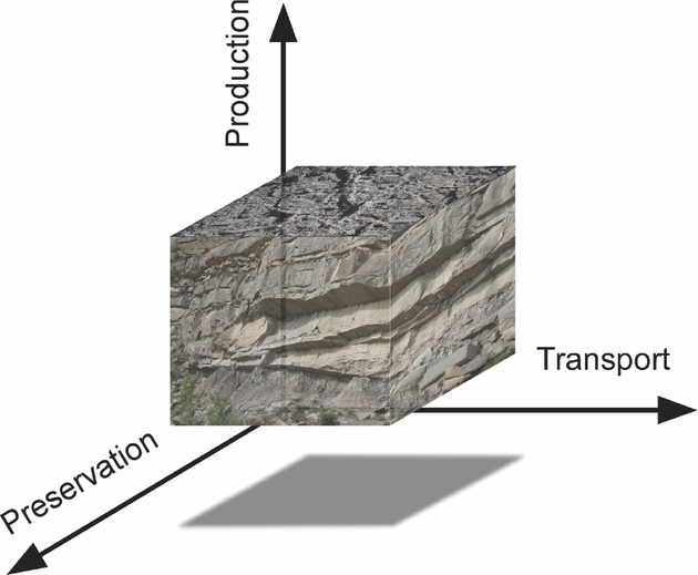
Figure 11. The concept of depositional space used in the lithofacies retrodiction method outlined in this paper. The three axes are a simplification of the three process groups, production, transport and preservation. In reality, this space is much more complex.

Figure 12. A simplified lithofacies retrodiction model workflow. Red links relate to direct input from palaeogeography (topography, bathymetry, coastlines, rivers). Blue links show direct links to Earth system model output. Each process comprises sub-processes, which are not shown.
Deterministic models, such as Merlin (Bohacs, West & Grabowski, Reference Bohacs, West and Grabowski2010; Harris et al. Reference Harris, Ashley, Otto, Crossley, Preston, Watson, Goodrich, Team, Valdes, AbuAli and Moretti2017), use values for each process based on a conditional statement determined from an analysis of observations, usually present-day relationships. The results are a series of spatial grids of 1’s and 0’s that can be weighted according to the ‘importance’ of each process. Since this ‘importance’ is not always known, weighting is avoided initially. Grids are then added or subtracted according to whether they act positively or negatively to the formation of source or reservoir facies. This is something akin to CRS (Common Risk Segment) mapping and can be similarly traffic-light coded, based on which processes are present or absent.
This method has two strengths: (1) it is simple, and (2) the method is transparent, meaning that the contribution of each process, and its significance in each retrodiction, can be assessed.
An alternative method assigns either a value and/or probability to each process based on a range of probable values (Markwick & Valdes, Reference Markwick and Valdes2007; Markwick, Gill & Valdes, Reference Markwick, Gill and Valdes2008). Probabilities can also be assigned using a Monte Carlo approach.
In both methods, the sensitivity of the system can be examined by changing the boundary conditions or input equations to answer ‘what if’ questions: if upwelling is switched off does this preclude a source facies? If the seasonality of stratification changes, what happens? This flexibility is a key advantage of such a transparent approach where each process can be examined and there is no pre-conceived bias, such as assuming the need for anoxia. Different systems will respond differently given different inputs, but all permutations might result in a source rock or reservoir. It is about knowing what you need to do to change the exploration risk of each play component and how likely that is.
The results of applying one set of criteria to the workflow for the Maastrichtian period are shown in Figure 13 for POC (particulate organic carbon) and for clastic grain size. In this specific organic matter scenario, values of productivity have been assigned to production and a burial efficiency value has been added for preservation to get relative values of POC, which can be compared with observations. This is just one scenario used as an example.

Figure 13. Lithofacies retrodiction results for the Maastrichtian period. (a) Particulate organic matter (POC %). (b) Potential clastic grain size determined by motion on the shelf. In this example, it is assumed that clastic sediments of the right grain size are available to be moved, but this can be further investigated by the output of the transport part of the models. Relative calculated sediment flux values are shown by pie charts for each mapped palaeo-river using empirical equations based on published databases (Meybeck, Reference Meybeck1976; Milliman & Syvitski, Reference Milliman and Syvitski1994; Hovius & Leeder, Reference Hovius and Leeder1998; Markwick et al. Reference Markwick, Proctor, Valdes, Wolf and Jacques2006). Lithological data and climate proxies from the Paleogeographic Atlas Project (Ziegler et al. Reference Ziegler, Rowley, Lottes, Sahagian, Hulver and Gierlowski1985, Reference Ziegler, Eshel, Rees, Rothfus, Rowley and Sunderlin2003) are shown to illustrate the density of data used to test and refine both the lithofacies retrodiction and Earth system models. This example only shows the results of one experiment.
Global palaeogeography plays a critical part in all stages of this workflow. It acts as the primary boundary condition for the Earth system modelling, which must initially be run globally given the interplay of the physics. It then provides direct inputs into the lithofacies models, including values for topographic relief, drainage basin and river geometries, distance from shorelines and river mouths, palaeo-canyons, and geographic and bathymetric restriction.
The coupled ocean–atmosphere models provide the climatology, oceanography and surface state (runoff, soil moisture, vegetation) and are generally run at a ‘coarse’ spatial resolution. The HadCM3 model (Pope et al. Reference Pope, Gallani, Rowntree and Stratton2000), which is used in this case study, has an atmospheric grid cell resolution of 3.75 × 2.5 degrees, and an ocean resolution of 1 × 1 degrees. Consequently, the input palaeogeographies do not need the same level of resolution as, say, regional- or play-scale maps. Much more important is being able to run sensitivity experiments to assess the implications of variability and uncertainty in the boundary conditions and test hypotheses. Markwick & Valdes (Reference Markwick and Valdes2004) used a grid resolution of 0.5 × 0.5 for their palaeoDEMs to be used with the HadCM3 model, which enabled the modellers to assign the variability in elevation within a model grid cell (Markwick, Reference Markwick, Williams, Haywood, Gregory and Schmidt2007). An analysis of the decorrelation distances of key climate variables also indicated the validity of using this resolution (Markwick, Reference Markwick, Williams, Haywood, Gregory and Schmidt2007). Other Earth systems models may require different resolutions; for example, the ICOM (Imperial College Ocean Model) tide model (Wells et al. Reference Wells, Allison, Hampson, Piggott and Pain2005) uses a variable mesh rather than a fixed grid cell size, with the grid resolution varying depending on where the computational detail is needed. This means that this sort of model can use higher resolution inputs and can be used at the regional and even basin scale when required in the exploration workflow.
The veracity of using global models and geographies has been questioned given their coarse resolution. However, the results of modelling experiments have indicated that the large-scale response of the Earth system is less sensitive to changes in palaeogeography at this resolution (whether due to uncertainty or variability) than to changes in atmospheric chemistry. But, those palaeogeographic changes do affect regional climatology and oceanography, especially through gateway changes (Lunt et al. Reference Lunt, Farnsworth, Loptson, Foster, Markwick, O'Brien, Pancost, Robinson and Wrobel2016). This would indicate that global palaeogeography can be used for first-order retrodictions of depositional play elements to high-grade basins or parts of basins, but that sensitivity experiments to constrain palaeogeographic variability and uncertainty at regional to local scales are essential. Getting the palaeodrainage correct is found to be very important. At the global scale, this is about defining the outfall point (river mouth) and drainage basin geometry; the details of the network are less important at this resolution. Deep-water palaeobathymetry is robust at all scales, but the palaeobathymetry of shelf areas, including epicontinental seas, can be problematic. Ocean gateways have a major effect on, especially, regional climatology and oceanography, and are a function of the plate model. This requires examining tectonic and biogeographic data. Again, sensitivity experiments can help assess the impact of these. Palaeotopography is probably the largest source of uncertainty in palaeogeographies. At global scales the key is to get the location, geometry (barrier or plateau) and approximate height (500 m or 1000 m or 2000 m or higher). Again, variability and uncertainty can be assessed using sensitivity experiments. Features such as lakes are best represented at a regional, basin and play scale given their sensitivity to local tectonics and hydrology, although generalizations can be made at a global scale to get first-order predictions for lithofacies modelling using process models such as those of Katz (Reference Katz and Huc1995) or Carroll & Bohacs (Reference Carroll and Bohacs2001).
4.b. Regional- to basin-scale exploration and palaeogeography. Case 2: drainage analysis and source-to-sink evolution of Cameroon and Gabon
Regional palaeogeographic maps share many of the same applications and issues as global-scale maps, but with a higher temporal and spatial resolution. Regional maps are largely used by asset teams who are focused on a margin or country and who are charged with building up a geological model (Fig. 1) or answering questions that have arisen from that model during exploration (Table 3). Like global maps, regional maps are also time consuming to build, but because of the increase in resolution, other issues become important (Table 3).
Table 3. Pros and cons of regional-scale palaeogeographic maps in exploration

This case study shows how regional- to basin-scale palaeogeography is used as part of a source-to-sink analysis along the West African margin from Cameroon to Congo. Two results are provided that reflect the different end-member methodologies used for reconstructing palaeodrainage as part of the palaeogeography workflow (Fig. 8): (1) Barremian syn-rift: working forwards in time using analogues, provenance data, palaeogeography and structural mapping; (2) Late Cretaceous post-rift: working backwards in time using drainage and landscape analyses, palaeobiogeography and provenance analysis.
4.b.1. Nature of the problem
The West African margin is a relatively mature exploration area (Teisserenc & Villemin, Reference Teisserenc, Villemin, Edwards and Santogrossi1989; Brownfield & Charpentier, Reference Brownfield and Charpentier2006), but questions and opportunities remain, especially in the pre-Salt (Hodgson, Rodriguez & Intawong, Reference Hodgson, Rodriguez and Intawong2017). Source rock questions revolve around understanding variations in the syn-rift lake systems and how these affect source facies distribution and quality; the lakes are a function of the geometry of accommodation space, which in large part is driven by the pre- and syn-rift crustal architecture (Karner et al. Reference Karner, Driscoll, McGinnis, Brumbaugh and Cameron1997), drainage interconnectivity and climate. Aptian salt acts as a seal for the pre-rift plays, but also as a trapping mechanism, but its extent, composition and thickness vary along the margin from the Gabon Basin north to the Douala Basin, again a function of the climate, accommodation space, depositional environment and freshwater flux. But, it is the clastic reservoirs in both syn-rift and post-rift plays that are most problematic with uncertainties about the continuation and composition of the Upper Cretaceous turbidites, and the distribution, porosity and permeability of the syn-rift Dentale Sandstone (Brownfield & Charpentier, Reference Brownfield and Charpentier2006). This requires an understanding of hinterland evolution and palaeodrainage reconstruction.
4.b.2. Reconstructing post-rift palaeodrainage starting with drainage network analysis
The problem is that there is a range of radically different hypotheses for the evolution of the river systems and corresponding palaeolandscapes along this margin. For the post-rift story, these are mostly focused on the history of the Congo River (Fig. 14). This has been partly driven by a perceived belief that large volumes of sediment in the offshore can only be explained by a large hinterland drainage: for example, the proposed past connection between the Congo River and the Ogooue River. Markwick & Valdes (Reference Markwick and Valdes2004) considered this to be an over-simplification and that the large volume of sediment in the Cretaceous Ogooue delta could be explained by the increased sediment flux resulting from uplift of the Gabon craton associated with the ‘Santonian inversion’.

Figure 14. Alternative hypotheses for the drainage evolution of the palaeo-Congo River. 1 – Northward into the Benue Trough and Chad Basins during the Cretaceous Period (Ziegler & Rowley, Reference Ziegler, Rowley, Crowley and Burke1998) based on micro-diamond provenance and palaeo-current directions in the Albian–Maastrichtian Carnot and Mouka-Ouadda Sandstone formations in the Central African Republic (Giresse, Reference Giresse1982, Reference Giresse1990, Reference Giresse2005; Censier, Reference Censier1990; Censier & Lang, Reference Censier and Lang1999). 2 – Karner & Driscoll (Reference Karner, Driscoll, Cameron, Bate and Clure1999) and Nibbelink & Budihardjo (Reference Nibbelink and Budihardjo2002) postulated that the palaeo-Congo River flowed into the palaeo-Ogooue River (probably via the Ivindo catchment) during the Cretaceous Period, in order to explain the large volume of Upper Cretaceous sediment along the northern margin of Gabon (Séranne & Anka, Reference Séranne and Anka2005). This forms the submarine distal fan of a postulated large, Late Cretaceous delta system. Karner & Driscoll (Reference Karner, Driscoll, Cameron, Bate and Clure1999) argued that flexural uplift of the margin then led to the migration of this river system south to its present location. Leturmy, Lucazeau & Brigaud (Reference Leturmy, Lucazeau and Brigaud2003) proposed a variation of this hypothesis with the Oubangui River, a northern tributary of the modern Congo River, flowing west into the palaeo-Ogooue River. 3 – Exit to the Atlantic through the present-day Congo River mouth since at least Late Cretaceous time (Anka, Séranne & di Primio, Reference Anka, Séranne and di Primio2010). 4 – Goudie postulated that the southern part (at least) of the palaeo-Congo River system drained into the palaeo-Limpopo River during the Cretaceous Period (Goudie, Reference Goudie2005). 5 – Stankiewicz & De Wit (Reference Stankiewicz and De Wit2006) proposed a Cretaceous connection into the Rufiji River in East Africa via the Rukwa Basin. 6 – Northeast connection into the Lamu Embayment during Middle and Late Jurassic times (Ziegler & Rowley, Reference Ziegler, Rowley, Crowley and Burke1998).
The first stage of any drainage reconstruction is to analyse the present-day drainage networks and landscape. These methodologies have been discussed in Markwick & Valdes (Reference Markwick and Valdes2004) and more recently by Markwick (Reference Markwick2013), who also showed the results for the West African margin, which are summarized in Figures 15 and 16a. This analysis shows evidence of river captures and flow reversals consistent with late Cenozoic uplift and southward tilting of the Gabon craton. The mechanism for this tilting is postulated to be related to the uplift of the mountains of northern Cameroon that mark the Oligocene–Recent Cameroon Volcanic Line (Gallacher & Bastow, Reference Gallacher and Bastow2012). During the same time interval, Africa is also uplifting in response to interpreted broader mantle processes referred to collectively as the ‘African Superswell’ (Nyblade & Robinson, Reference Nyblade and Robinson1994; Lithgow-Bertelloni & Silver, Reference Lithgow-Bertelloni and Silver1998; Gurnis et al. Reference Gurnis, Mitrovica, Ritsema and Van Heijst2000) but which encompasses a complex evolution of uplifts and subsidence (Moucha & Forte, Reference Moucha and Forte2011). This dynamic topography adds a further complexity to palaeogeography, as also indicated by fission track analysis (Harris et al. Reference Harris, Hegarty, Green and Duddy2002).
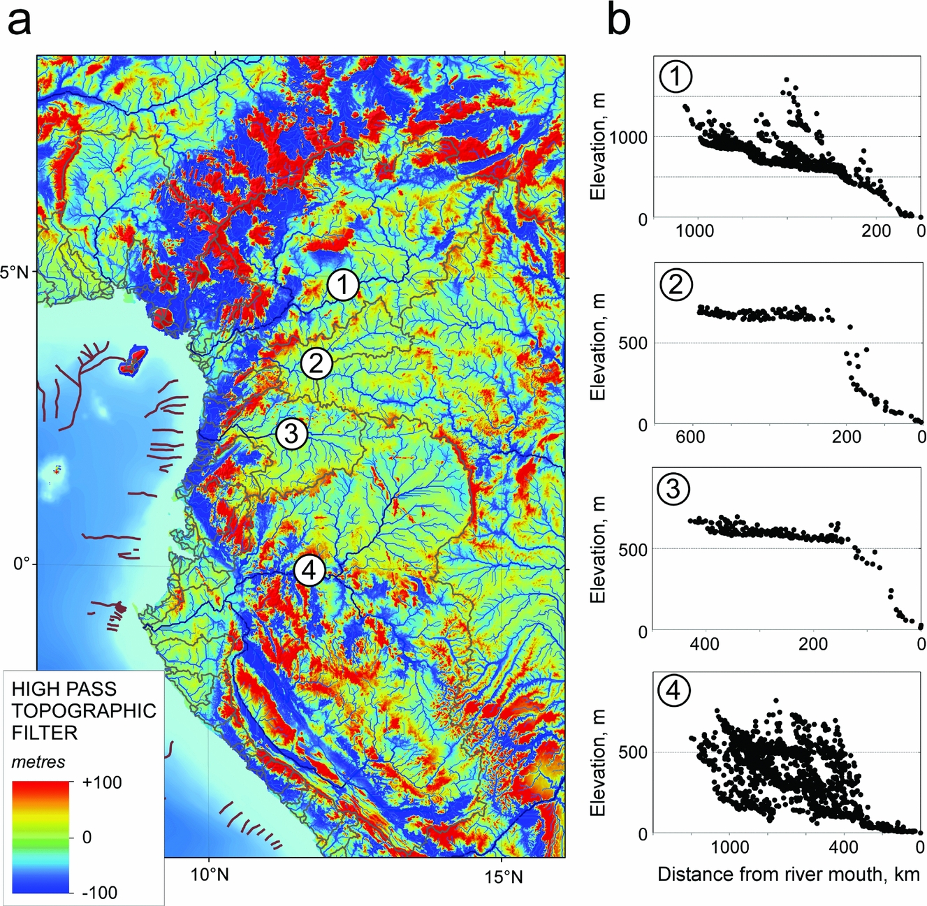
Figure 15. The key components of drainage and landscape analyses for the major rivers from Cameroon to Congo. (a) A high pass topographic filter to show topographic relief and areas of incision (increased incision marked by darker shades of blue). Across the Gabon craton, the major incision direction is to the north consistent with the southward tilting of this Precambrian cratonic block resulting from Oligo-Miocene uplift of the Cameroon Highland area. (b) River long profiles for the four principal rivers of this area: 1 – Sanaga River; 2 – Nyong River; 3 – Ntem River; 4 – Ogooue River. The Ntem and Nyong rivers show a raised ‘equilibrium profile’ (marked by the shallow, concave-up trend); the step pattern of the Sanaga River profile is consistent with capture of watersheds each marked by an ‘equilibrium profile’; the Ogooue River long profile shows no systematic pattern, which is consistent with recent capture of separate, previously independent drainage basins. Each basin long profile can be broken down further to assess internal trends and interpretations.

Figure 16. Drainage analysis results for major rivers from Cameroon to Congo. (a) The main trends of the present-day rivers (dark blue lines) and drainage divides (dashed red lines). Evidence for reversed flow of the headwaters of the Nyong River, indicated by barbed confluences, is consistent with the capture of these headwaters by the Congo River due to the uplift of the Gabon craton. Similar evidence of capture is seen in the headwaters of the Ntem River, but in this case, capture is by the Ogooue River via the rapidly expanding Ivindo catchment. (b) The interpreted palaeodrainage pattern indicated by analysing the present-day drainage network patterns, indicators of flow change, incision patterns (high pass filter), hypsometric curves (not shown here), river long profiles, geology and structure. This is interpreted to represent the pre-Oligocene palaeodrainage, on the basis that the uplift that has resulted in the interpreted changes is Oligo-Miocene in age. These results can then be added to the palaeogeographies for the pre-Oligocene and taken back to the last thermo-mechanical event.
Assuming the cause of the present-day networks is Oligocene to Recent uplift, then unwinding these network changes gives the pre-Oligocene drainage networks and palaeodrainage divides and the palaeo-hypsometry of the corresponding palaeolandscape. This reconstructed pre-Oligocene network comprises a series of parallel rivers running east to west (Fig. 16b), many picking out the traces of Precambrian shear zones, the palaeo-Ntem, -Sanaga and -Nyong rivers, or Precambrian lithological differences reflecting contemporary Precambrian basin geometry, such as the southern Ogooue River flowing from the Franceville Basin. This pre-Oligocene network shows no connection with the Congo River. These results are in agreement with the provenance analysis of Séranne, Bruguier & Moussavou (Reference Séranne, Bruguier and Moussavou2008), who concluded that the major incision seen today is relatively recent (no older than Oligocene) and that during much of the post-rift period denudation rates were low, consistent with no major elevation. This is also consistent with the study of Paul, Roberts & White (Reference Paul, Roberts and White2014), who postulated a relatively ‘flat’ Africa by Eocene time using drainage profile inversion methods, although with no definition of how flat is ‘flat’. The question is then how far back in time can this pre-Oligocene network be taken? Assuming low denudation rates and that the pre-Oligocene network and palaeolandscape is the product of the last tectonophysiographic (thermo-mechanical) event to affect the area, which is the ‘Santonian Inversion’, then this network can logically be extended back into the Late Cretaceous period (Figs 16b, 17b). This would suggest a slightly different nature to the Late Cretaceous uplift compared with that of the Oligocene–Recent, with a probable lack of asymmetry in the Gabon craton uplift such that the parallel river systems were maintained. An alternative hypothesis is that the palaeolandscape was eroded flat from Maastrichtian to Oligocene times and the drainage system was ‘reset’ to be defined by the parallel systems following the Precambrian structural fabric.

Figure 17. Drainage evolution of Cameroon to Congo during the Cretaceous Period. (a) Barremian syn-rift reconstruction of the palaeolandscape and palaeodrainage of the northern South Atlantic. The reconstruction of palaeo-rivers along each rift is conceptual with short-headed rivers draining into an axial trunk stream. Connectivity between individual rifts will evolve through time. The provenance of the Dentale Formation in the South Gabon Basin is equivocal, but the source shown here (blue arrows) from the north is consistent with the conclusion of Hodgson (Reference Hodgson2014). The high porosity and permeability reflect the consequences of longer distance reworking than would be expected were the sandstones sourced from adjacent rift shoulders. The map shows lakes more typical of the Melania Shale, which immediately underlies the Dentale sandstones. (b) Maastrichtian palaeodrainage reconstruction showing the uplifted Gabon craton, probably in response to the Santonian Inversion. Elevations are nonetheless relatively subdued. At this time the Cuvette Centrale is shown as erosional (the sub-Paleocene unconformity of Sachse, Delvaux & Littke, Reference Sachse, Delvaux and Littke2012).
4.b.3. Reconstructing syn-rift palaeodrainage using analogues and provenance indicators
For the drainage reconstructions older than the last thermo-mechanical event affecting the hinterland, the workflow relies more heavily on palaeo-current and provenance data as well as analogues rather than network analysis (Fig. 8). In the Lower Cretaceous of West Africa, palaeo-current indicators in the Cuvette Centrale suggest the presence of a major S–N-flowing river system, which requires a palaeodrainage divided between this palaeo-Congo and the rifting Atlantic basins. Within the rift basins, drainage networks are based on analogues and models (Gawthorpe & Leeder, Reference Gawthorpe and Leeder2000). In the absence of other information, sediment input points into the rifts from the hinterland are assumed to be through major transfer zones, some of which correspond to the shear zones that dictate the rivers today and the pre-Oligocene network. This is shown in Figure 17a. This palaeogeography must be consistent with subsequent timeslices, including the Late Cretaceous reconstructed drainage (Fig. 17b), pre-Oligocene network and the present day. This provides a check on what hypotheses are permissible.
4.b.4. Adding palaeoclimate, vegetation and bedrock
To complete the source-to-sink inputs, the climate, vegetation and bedrock are added (Fig. 18) to the reconstructed palaeolandscape and palaeodrainage and analysed in terms of sediment transport models, sediment composition and landscape stability (Langbein & Schumm, Reference Langbein and Schumm1958; Hovius & Leeder, Reference Hovius and Leeder1998; Syvitski et al. Reference Syvitski, Peckham, Hilberman and Mulder2003; Fraticelli et al. Reference Fraticelli, West, Bohacs, Patterson and Heins2004; Heins & Kairo, Reference Heins, Kairo, Arribas, Critelli and Johnsson2007) (Fig. 18).

Figure 18. Palaeo-geology and climate for the Late Cretaceous period of the Cameroon and Gabon area. (a) Surface geology rotated to the Maastrichtian as palaeo-geology. The margin is dominated by a hinterland comprising Precambrian granites and gneisses. The differential erosion of the Ogooue River reflects the location of the metasediments of the Franceville Basin (Ledru et al. Reference Ledru, N'Dong, Johan, Prian, Coste and Haccard1989), which then affects the compositions of clastic sediments sourced from this region. (b) Monthly modelled precipitation (blue columns) and mean temperature (red line) for the palaeo-Ogooue River and palaeo-Benue River. The palaeoclimate of this region in Maastrichtian time also affects sediment calibre. In Gabon, the Late Cretaceous climate is semi-arid with a seasonal rainfall potentially as flash floods. The semi-arid climate may have limited chemical weathering. To the north in northern Cameroon and Nigeria, the palaeo-ITCZ resulted in much wetter conditions, though still with a demonstrable seasonal signal in the palaeo-Benue drainage basin. This change in climate would be expected to affect vegetation and soil cover, with the concomitant stability of the landscape, especially on the flatter top to the Gabon craton. Slope failure along a developing coastal escarpment, especially in the wetter north, may have led to more clay-rich materials as are seen along the equatorial margin at this time.
In this example, the West African margin from Cameroon to Congo sat at the boundary between the equatorial wet zone of the ITCZ (Inter-Tropical Convergence Zone) and the arid trade wind belt to the south during much of the Cretaceous Period. Climate modelling has indicated that this hydrological zonation was intensified during the hot-house intervals, with Markwick, Crossley & Valdes (Reference Markwick, Crossley and Valdes2002) reporting runoff rates for the Late Cretaceous period of 2.5 times those for the present day, using a 4 times pre-Industrial CO2 experiment. Climate and relief from the palaeogeography also provide information on the nature of the erosion, whether this is through slope failure, flash floods, seasonal changes or extreme events, all of which will have a different sedimentological signature in the depocentre and also different compositional, porosity and permeability signatures in resulting reservoirs. Material dumped onto the shelf from the mapped palaeo-rivers was then subject to movement by tides, waves and ocean currents, which can also be modelled.
4.c. Basin- and play-scale exploration and palaeogeography. Case 3: palinspastic restorations and high-resolution palaeogeography in defining the central Pyrenees deep-water turbidites
At basin and play scales, palaeogeography is just one of a range of mapping tools available. At this point in the exploration pyramid (Fig. 1) the challenge is to identify and evaluate blocks and ultimately identify prospects, with more data and higher spatial and temporal precision (Table 4).
Table 4. Pros and cons of basin- and play-scale palaeogeographic maps in exploration

In this case study, the focus is on the restoration of the early Eocene (Ypresian) palaeogeography of the central Pyrenees to demonstrate how all the different components of the Earth system can be brought together in a rapidly changing palaeolandscape using high-resolution palaeogeography as the base/platform. This example permits an evaluation of the consequences of palinspastic restoration and mapping at higher temporal resolutions. The resulting map is constrained by field observations and designed to provide an analogue for exploration.
4.c.1. Nature of the problem
The Eocene of the central Pyrenees is a tectonically active area with rapid changes in structure, landscape and deposition. Deformation occurs in all dimensions, which creates problems for high-resolution palaeogeographic mapping used as the context for trying to fully explain the deep-water sandstone turbidites that are used as analogues in frontier areas such as the South Atlantic.
The central Pyrenees comprise the results of both thin-skinned and thick-skinned tectonics. These have a different expression in the landscape today, as they would have done in the past. This reflects observations that can be made in the field that show how each part of the compressional system behaves differently: some thrust sheets deform internally, some do not. This response appears to depend on the pre-existing structural fabric that is, or is not, inherited, and the ability of each thrust sheet to slide on the decollement surface, which in most parts of the central Pyrenees is Triassic salt (the distribution of salt is not uniform and is a function of Triassic palaeogeography). Again, this comes down to scale. Overall, the most southerly thrust sheet, the Serres Marginalis, has moved c. 60 km south since middle Eocene time (Muñoz et al. Reference Muñoz, Beamud, Fernández, Arbués, Dinarès-Turell and Poblet2013). This is superimposed on an overall crustal shortening of between 100 and 160 km in the central Pyrenees (Labaume et al. Reference Labaume, Meresse, Jolivet, Teixell and Lahfid2016). Restoration is further complicated by the associated rotation of features in the southern Ainsa Basin (Muñoz et al. Reference Muñoz, Beamud, Fernández, Arbués, Dinarès-Turell and Poblet2013) that must be reconstructed in the palaeogeography because they form positive bathymetric features that then affect the transport of clastic sediments to the deep-water margin, as well as acting as local sediment source areas.
4.c.2. Palinspastic reconstruction
The workflows at the basin and play resolution are the same as that described in Section 3 starting with the definition of the present-day structural framework and crustal architecture (Fig. 19). This is then queried for the early Eocene period, for which the active structures and geodynamics are shown in Figure 20. The difference in this example is that the deformation of each thrust sheet must be unravelled to generate a palinspastic solution (Fig. 20b), in this case, restored using the deformation reported in Muñoz et al (Reference Muñoz, Beamud, Fernández, Arbués, Dinarès-Turell and Poblet2013). This is then used to generate the depositional, elevation and drainage maps (Fig. 21) and from these the landscape maps (Fig. 22) with which to start to better understand how the system works.

Figure 19. The crustal architecture of the central Pyrenees. (a) The structural framework based on Landsat imagery, fieldwork and the 1:400000 BRGM geology map of the Pyrenees (BRGM & IGME, 2008) constrained in detail by the IGME 1:50000 geology maps where these are available across the region. Each structure is attributed with its age of activation and kinematic history, where this is known. (b) The crustal type represented by the major thrust sheets. These are coloured here by their age of first fault activity, but this is not unequivocal. Late Cretaceous – Cotiella-Boixols; Nogueres; North Pyrenean Frontal Thrust. Early Eocene – Peña Montañesa – Montsec; North Pyrenean. Middle Eocene – Larra-Monte Perdido; Ainsa Oblique Zone. Middle and/or late Eocene – Serres Marginals; Sierres Exteriores; Oturia; Ordesa; Gavarnie.

Figure 20. The early Eocene thermo-mechanical state of the central Pyrenees. (a) Structural elements active or present in early Eocene time and influencing the landscape (present-day coordinates) and the geodynamics (last thermo-mechanical event) relative to the early Eocene period; (b) The restored geometry consistent with the data and reconstructions of Muñoz et al. (Reference Muñoz, Beamud, Fernández, Arbués, Dinarès-Turell and Poblet2013). In this example changes in shape have been manually calculated; the restored positions of the towns of Tremp and Graus on the Peña Montañesa – Montsec thrust sheet are shown for reference (red filled circles and italic names).

Figure 21. The difference between the late early Eocene palaeogeography compiled on (a) a rigid plate solution and (b) a palinspastic reconstruction. The largest scale consequence of using a ‘palinspastic’ solution is that the source-to-sink story is much more linear and the deep-marine environments in the Ainsa Basin are less restricted. This changes in early Lutetian time as the Serres Marginalis, Peña Montañesa – Montsec and Cotiella thrust sheets move south with concomitant rotation and deformation in the Ainsa Oblique Zone. The exact position of the town of Ainsa is not clear and has been removed from this map to avoid confusion (the restored positions of Tremp and Graus are approximate). For the legend for depositional systems see Figure 7 and the online Supplementary Material available at http://journals.cambridge.org/geo. The legend for the areas above contemporary base-level (sediment source areas) is that shown in Figure 20.

Figure 22. Summary figure showing how all the components interact in the early Eocene period to form the deep-water turbidites. All of the components of the problem are now present: the underlying tectonics; the palinspastic restoration; depositional systems; uplift and palaeodrainage. It is into this spatial context, with an understanding of climate and sediment transport, that informed retrodictions of reservoir character (composition, volume, porosity and permeability), volume and timing can be made. In this Pyrenean analogue example, the palaeogeography can be related back to the field observations, which are now in their original spatial (geographic) context. The three field examples shown here represent positions in the same late Ypresian source-to-sink story: Location 1 is the Cassistent Sandstone (Montañana Group), near Puente de Montañana, representing the terrestrial, prograding delta top by sheet sands, here poorly sorted, with an erosional base cutting large channels and interpreted as flood related (Mutti et al. Reference Mutti, Tinterri, di Biase, Fava, Mavilla, Angella and Calabrese2000; Ramacha et al. Reference Ramacha, Poyatos-Moré, Fernández and Oms2011), concomitant with the wetter conditions resulting from the uplift of the Axial zone at this time and a change from the semi-arid red-beds of the ‘Garumnian’ facies (Maastrichtian–Paleocene). These are coeval with the turbidites at Arro (location 2; the photo shows the thinner turbidites overlying a thick sandstone turbidite interpreted to define a major canyon system in early Eocene time). Locality 3 is Broto in the Jaca Basin and the distal turbidite lobe deposits.
4.c.3. Temporal resolution, stratigraphic precision and reconstructing events
At this spatial resolution, the temporal resolution becomes much more important, especially when looking at deposition at the scale of a turbidite channel system or complex. The stratigraphic nomenclature of the area is not unequivocal, not least because of the structural complexity and sparsity of fossil information. The stratigraphic scheme used here is that of E. B. Amorós (unpub. Ph.D. thesis, Univ. Barcelona, 2013). The final map (Fig. 22) is reconstructed to represent the maximum progradation of the Montanyana Delta system represented by the Castissent Sandstone in the Tremp Basin, passing west through the Charo Canyon (Millington & Clark, Reference Millington and Clark1995) and associated Arro sandstone turbidites in the Ainsa Basin, and ultimately the distal fan complexes at Broto in the Jaca Basin. This map resolution is getting closer to a ‘moment in time’ à la Kay (Reference Kay1945). This enables the maps to be used to understand the interplay of tectonics, landscape, climate and deposition and identify any key causalities that can be transferred to exploration in frontier areas at the play to prospect scale. In this case, the palaeogeography (Fig. 22) shows the relationship of the uplifting Montsec thrust to deflect originally southward-flowing rivers west towards the deeper parts of the foreland basin. Climatically this is a wetter interval compared with the earlier Maastrichtian–Paleocene aridity indicated by the ‘Garumnian’ red beds. This is consistent with the uplift of the Axial zone acting as a focus for precipitation, and the more general intensification of the hydrological system during the early Eocene warm phases. The Cassistent Sandstone (Montañana Group) (Fig. 22) comprises often poorly sorted, sheet sands with erosional bases cutting large channels in the landscape and interpreted as flood related (Mutti et al. Reference Mutti, Tinterri, di Biase, Fava, Mavilla, Angella and Calabrese2000; Ramacha et al. Reference Ramacha, Poyatos-Moré, Fernández and Oms2011). Debrites amongst the Arro turbidites (pers. obs.) indicate gravity failure along the shelf margin, perhaps driven by either seismicity or climate (floods).
By using well-constrained palaeogeography in this way, together with all the components of the Earth system, the full context of the deep-water sandstone turbidites in the Ainsa Basin and their relationship to changes in the hinterland relief and climate become much clearer, knowledge that can then be applied to other exploration areas.
5. Conclusions
Palaeogeography is one tool in the explorationists toolbox (Adams, Reference Adams1943) providing a context for managing, visualizing and analysing large and diverse geological datasets. But, despite 200 years of published maps, the full potential of palaeogeography remains largely under-utilized in exploration, with its most common use as backdrop imagery in presentations.
The aim of this study was to try and change this by showing how palaeogeography can be used in exploration to bring together diverse information to solve geological problems and mitigate geological risk in exploration. The history of palaeogeography provides the context for understanding how palaeogeography has developed and has been applied in the past. This provides insights into how it can be used today. To facilitate this a workflow has been developed that can be used to standardize map generation and visualization, and which includes the key elements of the Earth system required to solve most geological problems in exploration. The basic concepts of this workflow date back to at least 1873 but have rarely been applied in full. How palaeogeography is then used, the mapping resolution and content depends on where in the exploration workflow you are and the problems being solved. This was shown through three case studies illustrating applications at different map resolutions and different stages within exploration.
It was also stressed throughout this paper that whilst spatial databasing, especially the use of ArcGIS (ESRI, 2017), has provided powerful tools for building and analysing palaeogeographies and associated information, which can then be ported to other software, this data and knowledge must be underpinned by a systematic, robust audit trail. Suggested standard protocols were provided in this paper and are included in the accompanying supplementary material (online Supplementary Material available at http://journals.cambridge.org/geo). These provide a means of qualifying mapping uncertainty and variability within a mapped time interval, the consequences of which for exploration can, and are, being investigated through sensitivity experiments using Earth system and process-based lithofacies retrodiction models.
Palaeogeography is not just an image.
Acknowledgements
I am indebted to Tony Doré, Guido Meinhold and an unnamed reviewer for their reviews and patience, from which this paper greatly benefited. This research received no specific grant from any funding agency, commercial or not-for-profit sectors.
Supplementary material
To view supplementary material for this article, please visit https://doi.org/10.1017/S0016756818000468


