


1 Introduction
There is a long-standing interest in the motion of the ocean’s uppermost layer. The relationship between near-surface current and wind was identified quite early on as a crucial piece of this picture (Durst Reference Durst1924, e.g.). The shape of the wind-forced velocity profile is understood to change between different depth regimes (Spalding Reference Spalding1961). In the classic formulation, fluid velocity decays linearly within the millimetre-thick viscous sublayer (Prandtl Reference Prandtl1910), just below which the velocity falls as the logarithm of depth (Taylor Reference Taylor1916; von Kármán Reference von Kármán1939). Ocean surface waves both complicate and enrich the picture. The theoretical ground supporting their investigation was formed in the late 18th century, with the recognisable formalism of Airy and Stokes being established in the 19th century (Craik Reference Craik2004); 20th century advances in the representation of water wave hydrodynamic theory (Phillips Reference Phillips1977, e.g.) have rendered it into a digestible and accessible form. Ocean surface waves are understood to aid greatly in the mediation of momentum, heat and gas fluxes between air and sea (Melville Reference Melville1996; Drennan, Kahma & Donelan Reference Drennan, Kahma and Donelan1999; Sullivan & McWilliams Reference Sullivan and McWilliams2010). The particulars of this mediation are often explicitly described using large-eddy simulation (LES), for example (Sullivan & McWilliams Reference Sullivan and McWilliams2010; Yang, Meneveau & Shen Reference Yang, Meneveau and Shen2013; Sullivan et al. Reference Sullivan, Banner, Morison and Peirson2017; Hao & Shen Reference Hao and Shen2019). Wave hydrodynamic motions modulate the centimetre-scale waves which are the Bragg scatterers for microwave radar (Alpers & Rufenach Reference Alpers and Rufenach1979), enabling the remote measurement of wind, wave and current properties. Stokes drift, the net forward motion produced by ocean surface wave orbital velocities over many wave periods (Stokes Reference Stokes1847), is another key component of near-surface ocean current, being especially strong close to the air–sea interface. Understanding of these processes has been aided by developments of theory for the impact of wind and wave-induced drift on near-surface mass transport (Bowden Reference Bowden1953; Longuet-Higgins Reference Longuet-Higgins1953; Phillips Reference Phillips1977; Breivik, Janssen & Bidlot Reference Breivik, Janssen and Bidlot2014, e.g.). One direction of work has been the establishment of parameterisations for wind drift, some of which have become ubiquitous in the field of physical oceanography (Wu Reference Wu1975, e.g.). The motivations for this work are clear: Stokes drift has long been hypothesised to play an important role in upper-ocean mixing (Falkovich Reference Falkovich2009). Furthermore, it has been shown to substantially affect the small-scale dynamics (DiBenedetto, Ouellette & Koseff Reference DiBenedetto, Ouellette and Koseff2018) and large-scale transport patterns (Curcic, Chen & Özgökmen Reference Curcic, Chen and Özgökmen2016; Morey et al. Reference Morey, Wienders, Dukhovskoy and Bourassa2018; Pizzo, Melville & Deike Reference Pizzo, Melville and Deike2019) of buoyant material; this has been explicitly extended to the transport of microplastics (Isobe et al. Reference Isobe, Kubo, Tamura, Kako, Nakashima and Fujii2014; Brunner et al. Reference Brunner, Kukulka, Proskurowski and Law2015) and spilled oil (Le Hénaff et al. Reference Le Hénaff, Kourafalou, Paris, Helgers, Aman, Hogan and Srinivasan2012).
Within the laboratory, many observations have been made of turbulent and wave-coherent aqueous fluid motions very near to a wavy interface. Early approaches made use of hydrogen bubble plumes to capture the profile shape in and below the viscous sublayer; Mcleish & Putland (Reference Mcleish and Putland1975) showed that turbulent wind forcing reduces the rate of decay of current speed with depth. Okuda, Kawai & Toba (Reference Okuda, Kawai and Toba1977) described similar observations in which the long wave shape was taken into account, providing skin friction and viscous sublayer thickness as a function of wave phase through a novel conditional-averaging approach. The classic work of Cheung & Street (Reference Cheung and Street1988) made use of laser Doppler anemometry (LDA) in measuring mean, turbulent and wave orbital velocities within the upper centimetres of the water column. They found the current profile just below the viscous sublayer to be ‘essentially logarithmic’ in all conditions. Laboratory particle image velocimetry (PIV) measurements have greatly improved the quality of these types of measurements. The viscous sublayer PIV measurements of Peirson (Reference Peirson1997) found that Mcleish & Putland (Reference Mcleish and Putland1975) and Okuda et al. (Reference Okuda, Kawai and Toba1977) may have overestimated the magnitude of stress in the viscous sublayer. Analysis of laboratory measurements by Banner & Peirson (Reference Banner and Peirson1998) reinforced this point, demonstrating that wave form drag dominates tangential stress for strongly forced wind waves. Peirson & Banner (Reference Peirson and Banner2003) provided evidence that microscale breaking waves (often called microbreakers for short) are the primary generation mechanism of aqueous surface layer flows under low to moderate wind forcing. Siddiqui & Loewen (Reference Siddiqui and Loewen2010) made use of similar techniques coupled with conditional averaging to investigate the long wave phase-dependent flow properties, finding that orbital velocity magnitudes were much (≈50 %) smaller for waves below microbreakers. These techniques were also employed by Vollestad, Ayati & Jensen (Reference Vollestad, Ayati and Jensen2019), who found that microscale breaking leads to strongly enhanced subsurface turbulent kinetic energy dissipation downwind of the wave crest. On the air side of the interface, numerous laboratory-based observational studies (Veron, Saxena & Misra Reference Veron, Saxena and Misra2007; Buckley & Veron Reference Buckley and Veron2016, Reference Buckley and Veron2017, Reference Buckley and Veron2019) have provided exciting measurements in this vein, with wave-coherent and turbulent air-side motions extracted through application of PIV.

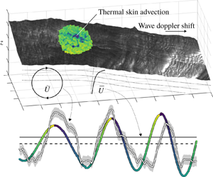
Figure 1. Stylised breakdown of the mean and wave orbital flow components  $\overline{U}$ and
  $\widetilde{U}$ underneath an undulating surface (in this case, the water surface displacement field produced through integration of the water surface slope field, supplemented with a representation of skin brightness temperature). The fixed and interface-following vertical coordinates
  $z$ and
  $\unicode[STIX]{x1D701}$ are shown for reference.
Measurements targeting mean and wave orbital velocities within centimetres of a wavy air–water boundary are rarely (if ever) made outside of the laboratory and in the real oceans. The undulating nature of the free surface presents a serious observational challenge: as shown in figure 1, one must describe both mean ( $\overline{U}$) and wave orbital flow components (
 $\widetilde{U}$) in a coordinate system which follows the air–sea interface. Some observational studies have recovered the mean current profile through the tracking of drifting instruments of varying depth, or draft (Stommel Reference Stommel1954; Bye Reference Bye1965; Churchill & Pade Reference Churchill and Pade1980; Churchill & Csanady Reference Churchill and Csanady1983; Bourassa Reference Bourassa2000). However, these are subject to scrutiny regarding the impact of direct windage on drifters of shallow draft. Wave orbital velocities have been measured via electromagnetic current meters (Bowden & White Reference Bowden and White1966; Thornton & Krapohl Reference Thornton and Krapohl1974) or (more recently) acoustic Doppler current meters (Herbers, Lowe & Guza Reference Herbers, Lowe and Guza1992, e.g.). However, acoustic Doppler current meters function quite poorly near to an undulating boundary (Nystrom, Oberg & Rehmann Reference Nystrom, Oberg and Rehmann2002). Even with such a sensor mounted on a long wave-following platform, flow distortion and instrument plunging would almost certainly contaminate many of the observations beyond use, making near-field remote sensing techniques optimal for near-surface current retrieval. Modern observations of near-surface ocean currents have largely been accomplished through radar remote sensing. High-frequency (HF) radar yields two-dimensional horizontal current fields in coastal regions, centred at between 1 and 2 m depth (Ardhuin et al. Reference Ardhuin, Marié, Rascle, Forget and Roland2009). Marine radar provides two-dimensional current fields with maximum range from the antenna typically varying between 2 and 4 km (Senet, Seemann & Ziemer Reference Senet, Seemann and Ziemer2001, e.g.); with additional processing, one may also obtain an estimate of the current profile to within ≈1 m of the sea surface (Lund et al. Reference Lund, Graber, Tamura, Collins and Varlamov2015, Reference Lund, Haus, Horstmann, Graber, Carrasco, Laxague, Novelli, Guigand and Özgökmen2018). Along-track interferometry (Romeiser et al. Reference Romeiser, Suchandt, Runge, Steinbrecher and Grunler2010) and Doppler scatterometry (Rodríguez et al. Reference Rodríguez, Wineteer, Perkovic-Martin, Gál, Stiles, Niamsuwan and Rodriguez Monje2018) represent the most sensitive of these radar techniques; like HF radar, they rely on the phase information of the scattered electromagnetic (EM) radiation, but for centimetre-scale ocean waves, enabling a sub-centimetre-depth measurement. Not all current remote sensing techniques involve radar; optical recovery of ocean surface wave signatures of length ≈1–10 m (Streßer, Carrasco & Horstmann Reference Streßer, Carrasco and Horstmann2017) has yielded promising estimates of the mean current velocity in the upper one metre of the sea. Recent advances in high-resolution camera and image processing techniques (Zappa et al. Reference Zappa, Banner, Schultz, Corrada-Emmanuel, Wolff and Yalcin2008, Reference Zappa, Banner, Schultz, Gemmrich, Morison, Lebel and Dickey2012) have opened the door to the study of the spatio-temporal behaviour of short waves of length ≈0.001–1 m from a single imaging enclosure. One application of this technology is the recovery of the current vector profile in the upper few centimetres of the water column (Laxague et al. Reference Laxague, Haus, Ortiz-Suslow, Smith, Novelli, Dai, Özgökmen and Graber2017), with some recent work establishing a proof of concept in the real ocean (Laxague et al. Reference Laxague, Özgökmen, Haus, Novelli, Shcherbina, Sutherland, Guigand, Lund, Mehta and Alday2018a).
The 2008 RaDyO (radiance in a dynamic ocean) field campaign saw the Research Platform R/P FLIP (“FLoating Instrument Platform”) moored off the coast of Santa Barbara (Zappa et al. Reference Zappa, Banner, Schultz, Gemmrich, Morison, Lebel and Dickey2012). The stability of FLIP coupled with the advanced sensor suite aboard during RaDyO made it an ideal candidate for a full application of the technique described by Laxague et al. (Reference Laxague, Haus, Ortiz-Suslow, Smith, Novelli, Dai, Özgökmen and Graber2017). A recent reanalysis of the RaDyO 2008 data set focused on the short wave spectral characteristics themselves (Laxague et al. Reference Laxague, Zappa, LeBel and Banner2018b). The present work takes a step in a different direction, combining measurements of thermal surface feature advection, short wave Doppler shift, and long wave phase to describe wave orbital and mean shear flows in the upper few centimetres of the sea. It is an opportunity to do in the real ocean what has been done for years in the laboratory (e.g. by Siddiqui & Loewen (Reference Siddiqui and Loewen2007) and predecessors) – to observe aqueous surface layer flow characteristics in order to better describe sea surface wave hydrodynamics and the physical transfer of momentum between the atmosphere and ocean. This will be parsed into two major categories: observations of the time-averaged current profile and observations of current which varies with long wave phase.
This study’s observations and processing techniques are described in § 2. Results are given and interpreted in § 3. The study’s conclusions are drawn in § 4.
2 Field observations and processing techniques
2.1 RaDyO 2008; standard wind and wave measurements
Observations were made in the Santa Barbara Channel from aboard the R/P FLIP during the 2008 radiance of the dynamic ocean (RaDyO) campaign. During RaDyO 2008, the main boom of R/P FLIP was outfitted with a number of sensors aimed at describing the sea state and quantifying air–sea fluxes; an overview of which – including its objectives, design, and broad results – is given by Zappa et al. (Reference Zappa, Banner, Schultz, Gemmrich, Morison, Lebel and Dickey2012). A more recent revisitation produced a study of centimetre-scale ocean surface roughness and its response to wind forcing (Laxague et al. Reference Laxague, Zappa, LeBel and Banner2018b); it will serve the reader as a useful reference for the details of how polarimetric slope sensing was applied to the polarised imagery data set. Furthermore, it provides a description of the background environmental conditions that provides context for the measurements described here. Over the course of the field campaign, 16 camera acquisitions were obtained which passed quality control. The present work borrows heavily from that study’s initial preparation of the data, although diverges in its particular analytical tools and ultimate presentation of results. Here, the focus is on the determination of current from the Doppler shifts of short gravity waves and the advection of thermal features in the ocean skin layer. These observations were reconciled with long wave phase information for the reconstruction of both wave orbital velocities and mean current shear.
The principal data streams used here (and by Laxague et al. (Reference Laxague, Zappa, LeBel and Banner2018b)) include the momentum flux computed from the sonic anemometer time series, the long wave water surface vertical displacement time series as obtained by LiDAR (light detection and ranging), the mean advection of skin temperature features as detected by infrared camera (§ 2.2) and the spatio-temporal evolution of decimetre to centimetre-scale ocean waves as measured by polarimetric camera (§ 2.4). A drawing representing the relative positions of these sensors is provided here as figure 2; note that the FLIP boom was 9 metres above the mean water level. The sonic anemometer used was a Campbell Scientific CSAT, which sampled the three-dimensional wind velocity vector at 20 Hz at the end of the FLIP boom. Using these data, the wind stress  $\unicode[STIX]{x1D749}$ was computed via eddy covariance (Edson et al. Reference Edson, Hinton, Prada, Hare and Fairall1998, e.g.). For the present work, this is represented in the form of the friction velocity
  $u_{\ast }=\sqrt{\unicode[STIX]{x1D70F}/\unicode[STIX]{x1D70C}}$ given fluid density
  $\unicode[STIX]{x1D70C}$, which is always air side here unless otherwise noted with an additional subscript (e.g.
  $u_{\ast w}$ for water side). The thermal infrared camera provided the measurement of mean horizontal fluid velocity in the ocean skin layer, as described in § 2.2 below.

Figure 2. Photograph of R/P FLIP (a) with the following components drawn for emphasis and labelled: (b) Polarimetric camera. (c) Infrared camera. (d) LiDAR. (e) Sonic anemometer. The LiDAR and anemometer mean freeboards are given as 9 and 10 m, respectively. Notice that the two camera fields of view and the LiDAR spot are collocated on the water surface.
2.2 Quantifying the advection of thermal skin features

Figure 3. Slice of a wavenumber–frequency spectrum produced from the infrared (IR) imagery in the downwind direction, with colour indicating spectral energy density (uncalibrated, but proportional to temperature2). The dotted line marks the slope of the SAS feature, from which the advective current of 29 cm s-1 was obtained. The dashed curves indicate the linear dispersion relation subjected to a current of 29 cm s-1. Note that wavenumber is given in cycles m-1 (not radians m-1), so the slope of the dotted line yields the advective current magnitude.
By invoking Taylor’s frozen turbulence hypothesis (Taylor Reference Taylor1938), it is possible to remotely infer the mean advective velocity of a fluid through quantification of the spatio-temporal evolution of turbulent eddies. This is most readily done in wavenumber–frequency space, as developed and introduced by Dugan & Piotrowski (Reference Dugan and Piotrowski2012) through three-dimensional (two spatial, one temporal) Fourier transforms of riverine flow optical video. In that work, a linear surface in the wavenumber–frequency spectrum well away from ocean wave dispersive features was shown to be the result of advection of turbulent eddies; it was termed the advective (or Taylor) surface. The direction of the advective current vector was also obtained, as the slope of this feature (in  $k{-}\unicode[STIX]{x1D714}$, or wavenumber–frequency, space) was estimated for each directional slice of the wavenumber–frequency spectrum. Later work by Brumer et al. (Reference Brumer, Zappa, Anderson and Dugan2016) used thermal imagery in the same way, this time recovering advection of features at the optical (e-folding) depth of the infrared radiation (≈10 μm). This current was described as being computed from ‘the advective surface in 3-D spectra of the skin temperature’, named SAS for short. There, the term ‘surface’ described the feature in the wavenumber–frequency spectrum which corresponded to turbulent eddies; its orientation in directional
  $k_{x}{-}k_{y}{-}\unicode[STIX]{x1D714}$ space indicates the flow velocity. In order to minimise confusion over terminology, for the remainder of this work, ‘surface’ will always refer to the air–sea interface. Here, we are chiefly concerned with flows in the upper centimetres of the ocean and thus made use of thermal imaging in order to obtain the true skin velocity as a reference surface current. The JADE 570 LWIR camera used during RaDyO allowed for the recording of ocean skin temperature to a 320 × 240 array at 60 f.p.s. It was positioned approximately 3.25 m from the end of the boom and angled at 20° from nadir. Its horizontal and vertical angles of view were 21.7° and 16.4°, respectively, resulting in a nominal image size of 2.5 m × 2.5 m on the water surface post-rectification. An example wavenumber–frequency spectrum computed from the JADE imagery is shown in figure 3. Notice that the SAS feature is far more prominent than the wave dispersion signature. This is due to the camera’s near-nadir (20°) incidence angle, an orientation which ensured high emissivity and therefore greater sensitivity to skin thermal features than to those reflected by the ocean surface.
2.3 Making use of the water surface vertical displacement measurements
On the underside of the boom, a downward-looking Riegl model LD90-3-3100VHS LiDAR was affixed, recovering the vertical displacement of the air–sea interface at 50 Hz. As the laser’s ≈10 cm footprint on the water and noise floor prevented its resolving anything which could be considered ‘high-frequency’ waves, a 1 Hz lowpass filter was applied to all LiDAR data.

Figure 4. Extraction of long wave phase and amplitude through the wavelet transform. (a) Typical snippet of water surface vertical displacement time series, with four 1/60 s windows marked as grey shaded regions. (b) Corresponding amplitude scalogram. (c) Corresponding phase wavelet scalogram. Colours in (a) and (c) correspond to long wave phase in radians, while colours in (b) correspond to long wave amplitude in metres. The red traces in (b) and (c) represent the time-period pairs of peak wavelet amplitude (as determined from (b)).
For the present work, the principal usefulness of the water surface vertical displacement data lies in their classification of the long wave phase. In order to recover this parameter throughout the observational record, a one-dimensional wavelet transform  ${\mathcal{W}}$ (Morlet et al. Reference Morlet, Arens, Fourgeau and Giard1982, e.g.) was applied to the water surface vertical displacement time series
  $\unicode[STIX]{x1D702}(t)$. The complex-valued output of this transform
  ${\mathcal{W}}[\unicode[STIX]{x1D702}(t)]$ describes the temporal variation of wave amplitude, frequency, and phase. An example of this approach’s utility is represented in figure 4, where a snippet time series of a water surface vertical displacement is shown coloured by the instantaneous phase of the dominant wave component as recovered from the wavelet transform. Using the long wave phase (
 $\unicode[STIX]{x1D711}$) and amplitude (a) obtained from the wavelet transform of the LiDAR time series, we compute the current as prescribed by deep water linear wave theory (from Phillips Reference Phillips1977)
 $$\begin{eqnarray}\widetilde{U}_{theory}(\unicode[STIX]{x1D701},\unicode[STIX]{x1D711})=a\unicode[STIX]{x1D714}\text{e}^{k\unicode[STIX]{x1D701}}\cos \unicode[STIX]{x1D711}.\end{eqnarray}$$
 Here,  $\unicode[STIX]{x1D701}$ is the interface-following vertical coordinate,
  $\unicode[STIX]{x1D714}$ is the wave angular frequency and
  $k$ is the wavenumber computed from the deep water gravity linear dispersion relation. Equation (2.1) will serve as a useful reference point for the observations in the analyses to come.
2.4 Measuring the Doppler shift of short gravity waves

Figure 5. (a) Polarimetric camera enclosure alongside sample water surface slope field (along-look component). (b) Orthorectified slope field, with frame corner positions determined by the instantaneous camera freeboard and three-dimensional attitude using the transformation matrix given in (2.2).
The polarimetric camera was positioned 7 m back from the end of the boom and angled at 37° from nadir such that its imaging field of view was collocated with the LiDAR footprint on the mean water level. The ‘polarimetric camera’ in fact consists of four individual JAI (model CV-A10CL M) cameras enclosed within a custom-built housing, sharing a single narrow field-of-view (FOV) lens (horizontal and vertical angles of view of 4.8° and 3.6°, respectively). Two polarising beamsplitters within the enclosure allow the device to obtain images of light at 0°, 45°, 90° and 135° polarisations with ≈1 ms sensor integration times, minimising the effect of motion blur (Zappa et al. Reference Zappa, Banner, Schultz, Gemmrich, Morison, Lebel and Dickey2012). By employing the polarisation slope sensing (PSS) technique (Zappa et al. Reference Zappa, Banner, Schultz, Corrada-Emmanuel, Wolff and Yalcin2008, Reference Zappa, Banner, Schultz, Gemmrich, Morison, Lebel and Dickey2012), the along and cross-look water surface slope was obtained at each pixel over the image at a sampling rate of 60 f.p.s. Validation data collected and presented by Zappa et al. (Reference Zappa, Banner, Schultz, Corrada-Emmanuel, Wolff and Yalcin2008) show that the root-mean-square difference between PSS slope and a reference point slope gauge was less than 0.5°. Boom/camera motion, although minimal to the point of being neglected in the wavenumber spectral analysis of Laxague et al. (Reference Laxague, Zappa, LeBel and Banner2018b) (rotational rates smaller than 1 deg s-1), was still substantial enough to affect the sensitive analysis performed here. In order to mitigate these effects, the data streams from the boom-mounted six degree-of-freedom inertial measurement unit and LiDAR were used for the full rectification of the polarisation imagery products. For a given slope field, the positions of its four corners were taken to be the heads of vectors originating from the camera’s focal point. At every time step, each of the vectors was multiplied by the three-dimensional rotation matrix given in (2.2) (following Anctil et al. (Reference Anctil, Donelan, Drennan and Graber1994), from Goldstein (Reference Goldstein1950)). Given the Euler angles  $\unicode[STIX]{x1D703}$,
  $\unicode[STIX]{x1D719}$ and
  $\unicode[STIX]{x1D713}$ corresponding to the camera’s instantaneous pitch, roll and heading, respectively, this matrix is as follows:
 $$\begin{eqnarray}\unicode[STIX]{x1D64F}_{R3}=\left[\begin{array}{@{}ccc@{}}\cos \unicode[STIX]{x1D703}\cos \unicode[STIX]{x1D713} & \sin \unicode[STIX]{x1D719}\sin \unicode[STIX]{x1D703}\cos \unicode[STIX]{x1D713}-\cos \unicode[STIX]{x1D719}\sin \unicode[STIX]{x1D713} & \cos \unicode[STIX]{x1D719}\sin \unicode[STIX]{x1D703}\cos \unicode[STIX]{x1D713}+\sin \unicode[STIX]{x1D719}\sin \unicode[STIX]{x1D713}\\ \cos \unicode[STIX]{x1D703}\sin \unicode[STIX]{x1D713} & \sin \unicode[STIX]{x1D719}\sin \unicode[STIX]{x1D703}\sin \unicode[STIX]{x1D713}+\cos \unicode[STIX]{x1D719}\cos \unicode[STIX]{x1D713} & \cos \unicode[STIX]{x1D719}\sin \unicode[STIX]{x1D703}\sin \unicode[STIX]{x1D713}-\sin \unicode[STIX]{x1D719}\cos \unicode[STIX]{x1D713}\\ -\text{sin}\,\unicode[STIX]{x1D703} & \sin \unicode[STIX]{x1D719}\cos \unicode[STIX]{x1D703} & \cos \unicode[STIX]{x1D719}\cos \unicode[STIX]{x1D703}\end{array}\right]\!.\end{eqnarray}$$
 The spatial extent of each slope field was obtained by computing the intersection of the rotated vectors with the plane  $z=-h+\unicode[STIX]{x1D702}$, where
  $h$ is the mean camera freeboard of 9 m and
  $\unicode[STIX]{x1D702}$ is the instantaneous water surface vertical displacement as measured by the LiDAR. An example of this orthorectification is represented in figure 5. This step was in keeping with a first-order assumption of a locally flat ocean solely for the purposes of rectification. Long wave steepness
  $ak$ varied between ≈0.01 and 0.1 radians, meaning that the second-order correction (a linearly tilted surface) would adjust the elevation of the frame corners by ≈0.5 %–5 % relative to the frame centre. This was deemed to be an acceptable level of deviation for the measurements made here. Once each slope field was orthorectified, it was subjected to a two-dimensional Tukey (tapered cosine) window in order to mitigate the contamination of spurious low-wavenumber signals resulting from the slope field’s abrupt edges; this was also performed on the slope fields analysed by Laxague et al. (Reference Laxague, Zappa, LeBel and Banner2018b).

Figure 6. (a) Directional wavenumber saturation spectrum computed over one second, with downwind direction indicated by the white line. Colour represents the base ten logarithm of saturation spectral density in radians. (b) Slice of the wavenumber–frequency spectrum in the downwind direction, normalised by the peak spectral density at each frequency. Solid, dot-dashed, and dotted lines: linear dispersion relation without current, same + 25 cm s-1 current, bound wave celerity of 73 cm s-1 (corresponding to a 34 cm wavelength).
The spatio-temporal arrays of water surface slope were zero padded along the spatial dimensions and then subjected to three-dimensional fast Fourier transforms in order to recover the wavenumber–frequency slope spectra  $S(k_{x},k_{y},\unicode[STIX]{x1D714})$. This process has become increasingly common in the study of ocean surface waves and the currents on which they propagate (Senet et al. Reference Senet, Seemann and Ziemer2001; Leckler et al. Reference Leckler, Ardhuin, Peureux, Benetazzo, Bergamasco and Dulov2015; Lund et al. Reference Lund, Graber, Tamura, Collins and Varlamov2015; Laxague et al. Reference Laxague, Haus, Ortiz-Suslow, Smith, Novelli, Dai, Özgökmen and Graber2017). Two products of a full wavenumber–frequency spectrum are seen in figure 6: in (a),
  $S(k_{x},k_{y},\unicode[STIX]{x1D714})$ was integrated with respect to positive frequencies in order to recover the true (unambiguous) directional wavenumber spectrum, here represented as
  $k^{2}S(k_{x},k_{y})=B(k_{x},k_{y})$. In (b), a wavenumber–frequency slice of the spectrum was taken in the downwind direction,
  $S(k_{d},\unicode[STIX]{x1D714})$. Of note: the gravity–capillary linear dispersion relation, indicated in the absence of current and in the presence of a 25 cm s-1 current in figure 6(b) as solid and dot-dashed lines, respectively. The dotted line of greater steepness represents the celerity of the bound waves seen for
  $k>125~\text{rad}~\text{m}^{-1}$. As bound waves are not simply advected by currents – but also by a dominant wave of larger scale (Plant et al. Reference Plant, Keller, Hesany, Kara, Bock and Donelan1999) – their presence on the ocean surface makes the recovery of near-surface currents through spectral techniques quite challenging. Past forays into this area (Laxague et al. Reference Laxague, Haus, Ortiz-Suslow, Smith, Novelli, Dai, Özgökmen and Graber2017, Reference Laxague, Özgökmen, Haus, Novelli, Shcherbina, Sutherland, Guigand, Lund, Mehta and Alday2018a) have avoided them entirely, neglecting portions of the spectra in which bound waves are present.

Figure 7. (a) Example wavenumber–frequency spectrum taken from one second of data, with downwind and upwind wave propagation indicated by positive and negative frequencies, respectively. The linear dispersion relation for  $U=0$ is given as a solid black line. (b) The difference between downwind and upwind wave celerity, computed from (a). In both panels, the vertical dashed line indicates the wavenumber at which bound waves become dominant, as indicated by the constant celerity in (a) and the constant difference in celerity in (b).
For each of the 16 data acquisitions, the slope field time series was partitioned into one second segments of time, with each segment overlapping by 0.5 s with both of its nearest neighbours. This is indicated by the grey shaded regions in figure 4(a). Temporal ‘shading’ was designed to squeeze the greatest possible number of individual Doppler shift estimates into a given long wave period while still retaining the ability to temporally resolve the longest waves captured in the nominally 1 m × 1 m camera footprint. Small variations in the dominant wave period ensured that the measurements made through this fixed-interval sampling were widely spread in long wave phase space. For each spectrum, the wavenumber position of peak spectral amplitude was determined at each wave frequency in both the downwind and upwind directions. A representation of this step is given in figure 7; the example cutoff wavenumber of 90 rad m-1 represents the limit below which we obtain usable data. This wavenumber varies by spectrum and marks the point at which the presence of bound waves prevents the recovery of current; note that  $\unicode[STIX]{x0394}C_{p}$ flattens out for
  $k>90~\text{rad}~\text{m}^{-1}$, potentially the result of this bound wave contamination. The approach performed here follows that of Plant & Wright (Reference Plant and Wright1980), in which the advecting current was determined from the difference in downwind and upwind wave celerities
 $$\begin{eqnarray}\displaystyle & \displaystyle C_{p,x}(k)=\frac{2\unicode[STIX]{x03C0}f_{x}}{k}, & \displaystyle\end{eqnarray}$$
 $$\begin{eqnarray}\displaystyle & \displaystyle \boldsymbol{U}(k)=C_{p,d}(k)\boldsymbol{e}_{d}-C_{p,u}(k)\boldsymbol{e}_{u}, & \displaystyle\end{eqnarray}$$
 where  $\boldsymbol{e}_{d}$ and
  $\boldsymbol{e}_{u}$ are the unit vectors corresponding to current in the downwind and upwind directional semicircles, respectively;
  $\boldsymbol{U}(k)$ is represented as a current profile
  $\boldsymbol{U}(\unicode[STIX]{x1D701})$ using the results of Plant & Wright (Reference Plant and Wright1980), where the surface-following vertical coordinate
  $\unicode[STIX]{x1D701}$ was computed using the equation
  $\unicode[STIX]{x1D701}=-0.044(2\unicode[STIX]{x03C0}/k)$. Laboratory measurements were performed by Laxague et al. (Reference Laxague, Haus, Ortiz-Suslow, Smith, Novelli, Dai, Özgökmen and Graber2017) in order to provide validation of this technique applied to short gravity wave spectra obtained from optical polarimetry. The root-mean-square (r.m.s.) difference between the wave spectral current estimate and the reference measurement – camera-tracked dye speed – was 3.4 cm s-1 across all laboratory measurements. This range is shown on the observed current time series given in figure 8(a).
2.5 Decomposing current into mean and wave orbital flows
In order to provide a more robust comparison of these current profile observations with wave hydrodynamic theory and past observations of surface layer fluid dynamics, the current time series were subjected to averaging which was conditional upon the long wave phase, thus preserving the phase-varying behaviour. This is sometimes referred to as ‘phase averaging’, although it is the phase which is being preserved, in contrast to the processes of ‘time averaging’ or ‘spatial averaging’ which collapse the data along the dimension in question. From here, the current profile at each time step was parsed in order to build a three-dimensional array which varies in time, depth and long wave phase. That block of data was subjected to a conditional time average, collapsing into an array which varies in depth and long wave phase (here termed ‘phasogram’) through the process represented in figure 8. We recall that the first wave crest depicted in figure 4(a) does not exactly match the zero phase indicated by the curve’s colour; however, this approach generally performs quite well at retrieving wave phase, as shown in figure 8(a).

Figure 8. (a) Example ten second time series of nearest-surface mean and wave orbital velocity components in the downwind direction as computed from the short wave Doppler shift; the coloured curve represents the value determined from the LiDAR data and linear wave theory (2.1). The grey shaded region about the observed current time series indicates the r.m.s. error for the technique, 3.4 cm s-1. (b) Visual representation of a phase-preserving time average which collapses a three-dimensional array of current measurements made over ten minutes into a two-dimensional phasogram.
For further analysis, we followed Benilov, Kouznetsov & Panin (Reference Benilov, Kouznetsov and Panin1974) and decomposed the raw phasogram into mean ( $\overline{\boldsymbol{U}}$) and wave orbital (
 $\widetilde{\boldsymbol{U}}$) components, neglecting the turbulent fluctuations which we cannot resolve
 $$\begin{eqnarray}\boldsymbol{U}(\unicode[STIX]{x1D711},\unicode[STIX]{x1D701})=\overline{\boldsymbol{U}}(\unicode[STIX]{x1D701})+\widetilde{\boldsymbol{U}}(\unicode[STIX]{x1D711},\unicode[STIX]{x1D701}).\end{eqnarray}$$
 Note that in contrast to Benilov et al. (Reference Benilov, Kouznetsov and Panin1974) (and more recently, Buckley & Veron (Reference Buckley and Veron2016, e.g.)), the total velocity phasogram does not need a coordinate transformation to enter an interface-following reference frame. This is a consequence of the fact that the short waves themselves (and, for SAS, the thermal skin features) are implicitly surface following; recall the coordinate system depicted in figure 1. The mean current profile  $\overline{\boldsymbol{U}}$ is itself composed of multiple elements. For the purposes of this work, we break this down into the following three components:
 $$\begin{eqnarray}\overline{\boldsymbol{U}}(\unicode[STIX]{x1D701})=\boldsymbol{U}_{b}+\boldsymbol{U}_{S}(\unicode[STIX]{x1D701})+\boldsymbol{U}_{i}(\unicode[STIX]{x1D701}),\end{eqnarray}$$
 where  $\boldsymbol{U}_{b}$ is the background Eulerian current,
  $\boldsymbol{U}_{S}(\unicode[STIX]{x1D701})$ is the Stokes drift profile and
  $\boldsymbol{U}_{i}(\unicode[STIX]{x1D701})$ is the ‘interface forcing’ (Laxague et al. Reference Laxague, Özgökmen, Haus, Novelli, Shcherbina, Sutherland, Guigand, Lund, Mehta and Alday2018a), i.e. the wind-induced near-surface drift which is directly attributable to viscous stress and microscale wave breaking.
2.6 Computing Stokes drift from long and short gravity waves
The RaDyO dataset contains measurements of wave characteristics at a wide range of scales, allowing for the spectral computation of Stokes drift, following Webb & Fox-Kemper (Reference Webb and Fox-Kemper2011, Reference Webb and Fox-Kemper2015). This was split into two segments, one making use of the LiDAR point surface displacement data and the other making use of the polarimetric slope field spatio-temporal evolution data. For the former, the omnidirectional elevation spectra  $E_{f}(f)$ were computed and trimmed in frequency space to yield an approximate wavenumber domain of
  $0.01<k<5~\text{rad}~\text{m}^{-1}$; an example is shown in figure 9(a). They were then subjected to the 1Dh-SD (one-dimensional Stokes drift) formulation of Stokes drift
 $$\begin{eqnarray}U_{S}\approx \boldsymbol{e}^{w}\frac{16\unicode[STIX]{x03C0}^{3}}{g}\int _{0}^{\infty }f^{3}E_{f}(f)\exp \left[\frac{8\unicode[STIX]{x03C0}^{2}f^{2}z}{g}\right]\text{d}f.\end{eqnarray}$$
 The fully directional wavenumber slope spectra were trimmed in wavenumber space to match the range of  $k$ used in the Doppler shift approach provided in § 2.4; an example dimensionless directional saturation spectrum is shown in figure 9(b). The slope spectra were used to produce the elevation wavenumber spectra
  $E(k_{x},k_{y})$, which were then converted to directional frequency spectra
  $E_{f\unicode[STIX]{x1D703}}(f,\unicode[STIX]{x1D703})$ following Plant (Reference Plant2009). Following this step, their contribution to Stokes drift was computed through the 2Dh-SD (two-dimensional Stokes drift) formulation:
 $$\begin{eqnarray}U_{S}\approx \boldsymbol{e}^{w}\frac{16\unicode[STIX]{x03C0}^{3}}{g}\int _{0}^{\infty }\int _{-\unicode[STIX]{x03C0}}^{\unicode[STIX]{x03C0}}(\cos \unicode[STIX]{x1D703},\sin \unicode[STIX]{x1D703},0)f^{3}E_{f\unicode[STIX]{x1D703}}(f,\unicode[STIX]{x1D703})\exp \left[\frac{8\unicode[STIX]{x03C0}^{2}f^{2}z}{g}\right]\text{d}\unicode[STIX]{x1D703}\,\text{d}f.\end{eqnarray}$$
 These two components were added together in order to produce the contribution from long and short gravity waves. The Stokes drift profiles computed from the long waves only and the combined data are shown in figure 9(c). The high-wavenumber cutoff serves multiple purposes, with three listed here. First – that all wave components represented in wavenumber space are resolved in frequency space in order to eliminate the 180° propagation ambiguity ( $f_{Nyquist}$ is the limiting factor, not
  $k_{Nyquist}$). Second – that there is not a great scale separation between the waves used to compute Stokes drift and those used to compute the Doppler shift; one would not expect the Stokes drift from 1 cm long waves to change the observed frequency of 10 cm long waves. Third – that the effects of capillarity do not greatly impact any of the results; this is essential when one relies on the gravity–capillary linear dispersion relation and the surface tension is unknown.

Figure 9. (a) Omnidirectional water surface elevation spectrum  $E(f)$ computed from the LiDAR time series. (b) Fully directional wavenumber saturation spectrum
  $B(k_{c},k_{d})=k^{2}S(k_{c},k_{d})$, with colour indicating the base-ten logarithm of saturation spectral energy density in radians. Subscripts
  $d$ and
  $c$ represent downwind and cross-wind directions, respectively. (c) Stokes drift profiles computed from the two spectra.
3 Interpretation of results
3.1 Mean current profile characteristics
Here, we present the results in two segments: one for the mean current profiles and one for the wave orbital flows. Selected environmental conditions from the cases described here are given in table 1.
The separation of observed near-surface current into mean and wave orbital components (as described in (2.5)) is graphically depicted in figure 10. There, the phase and depth-varying observed current is decomposed into the mean profile and the mean orbital phasogram. The mean current profile is shown alongside the SAS skin velocity magnitude,  $U_{S}$, computed as described in § 2.6, and a parameterisations of wind drift.
Table 1. Selected wind, wave and current conditions during the field observational campaign: ten metre neutral wind speed  $U_{10N}$ (m s-1), air-side friction velocity
  $u_{\ast }$ (cm s-1), peak surface gravity wave period
  $T_{p}$ (s), 100 times the wave steepness
  $ak$ (rad), 100 times the peak short wave growth rate
  $\unicode[STIX]{x1D6FD}_{p}$ (s-1) and the ocean skin velocity magnitude
  $U_{SAS}$ (cm s-1). Recall that these cases match those described in Laxague et al. (Reference Laxague, Zappa, LeBel and Banner2018b).


Figure 10. (a) Example decomposition of the total observed horizontal current phasogram ( $U$) into a mean depth-varying component (
 $\overline{U}$) and a wave orbital phasogram (
 $\widetilde{U}$). The teal dashed and black dotted curves in the middle panel represent the Stokes drift profile computed (Webb & Fox-Kemper Reference Webb and Fox-Kemper2011, Reference Webb and Fox-Kemper2015) for gravity waves with
  $k<5~\text{rad}~\text{m}^{-1}$ and
  $k<25~\text{rad}~\text{m}^{-1}$, respectively, while the × symbol represents the empirical surface wind drift as 3.5 % of the 10 m neutral wind speed (Wu Reference Wu1975). Colour indicates current velocity in cm s-1. (b) Depth-averaged current variation as a function of long wave phase; dominant wave direction is noted by the black arrow. Violet circles represent observations and the teal trace represents the result of linear wave theory given the LiDAR-obtained water surface vertical displacement measurements (2.1). The violet shaded region represents the interquartile range of observations.
Averaging the raw current phasograms over long wave phase yields the mean profile as obtained by short wave Doppler shift. Together with the SAS measurements, these provide current profiles like the one produced by Laxague et al. (Reference Laxague, Özgökmen, Haus, Novelli, Shcherbina, Sutherland, Guigand, Lund, Mehta and Alday2018a) with the added benefit of the skin (≈10 μm depth) velocity as a true surface current observation. We note that Stokes drift computed from LiDAR-measured waves is likely an overestimation of its true value. As no directional information was obtained for these waves, Stokes drift was computed assuming that all waves were propagating in one direction. While this is true for swell, spreading and multidirectional characteristics of wind sea (e.g. bimodality) work to make net forward transport smaller in reality than would be computed using a one-dimensional Stokes formulation (Webb & Fox-Kemper Reference Webb and Fox-Kemper2015).

Figure 11. Filled circles represent the observed current profiles in wall coordinates (Spalding Reference Spalding1961):  $u^{+}=(U_{0}-U(\unicode[STIX]{x1D701}))u_{\ast w}^{-1}$,
  $\unicode[STIX]{x1D701}^{+}=|\unicode[STIX]{x1D701}|u_{\ast w}\unicode[STIX]{x1D708}^{-1}$, where
  $u_{\ast w}$ is the water-side friction velocity and
  $\unicode[STIX]{x1D708}$ is the kinematic viscosity of water. RaDyO field observational data are coloured by air-side friction velocity
  $u_{\ast }$ in cm s-1. Black symbols represent laboratory observational data from Cheung & Street (Reference Cheung and Street1988): ▵ – 1.5 m s-1, ▿ – 2.6 m s-1, ▹ – 3.2 m s-1, ▫ – 4.7 m s-1, ♢ – 6.7 m s-1, ○ – 9.9 m s-1 (wind waves only). The solid coloured trace represents the laboratory observation of a current profile in a turbulent flow from Mcleish & Putland (Reference Mcleish and Putland1975). The red dashed curve represents the piecewise function describing the law of the wall (Spalding Reference Spalding1961).
The best way to examine these measurements together in the context of theory and previous studies is to represent them in wall coordinates (Spalding Reference Spalding1961); this is done in figure 11. Observed profiles are shown alongside the laboratory observations of Cheung & Street (Reference Cheung and Street1988) and a piecewise function for the law of the wall (Spalding Reference Spalding1961). This function is composed of relations originating from Prandtl (Reference Prandtl1910), Taylor (Reference Taylor1916) and von Kármán (Reference von Kármán1939). It describes the transition of the current profile from linear with depth in the viscous sublayer to logarithmic with depth in the layers immediately below. The depth assignment scheme for the short wave Doppler shift currents used here (from Plant & Wright (Reference Plant and Wright1980)) was generated with the assumption of a logarithmic profile shape. As such, it should not surprise that the profile behaviour for higher values of  $\unicode[STIX]{x1D701}^{+}$ tends to follow the logarithmic shape of the red dashed line. However, there are no assumptions made about the logarithm’s coefficient or offset, nor of the magnitude of the SAS current, all of which are strong determinants of the vertical level of
  $u^{+}$. The aqueous friction velocity was computed assuming viscous stress continuity across the air–sea interface:
  $u_{\ast w}=u_{\ast }\sqrt{\unicode[STIX]{x1D70C}/\unicode[STIX]{x1D70C}_{w}}$. As demonstrated in the laboratory measurements of Banner & Peirson (Reference Banner and Peirson1998) and the analysis of field measurements by Bourassa (Reference Bourassa2000), we expect form drag to constitute a fraction of the water-side stress that increases with the wind forcing. This means that the stress equivalence we assume would not hold, slightly changing the position and slope of the observed profiles. We do not believe that this potential disparity between estimation and truth is prohibitive, but it should be noted nonetheless.
Recent work by Teixeira (Reference Teixeira2018) drew from basic fluid mechanical theory to develop an analytical model for the current profile beneath a monochromatic water wave. The model inputs include wind forcing ( $u_{\ast }$), surface Stokes drift (
 $U_{S}(0)$) and the wavenumber of the surface wave (
 $k_{s}$); the non-dimensional turbulent Langmuir number is computed from two of these parameters and is expressed as
 $$\begin{eqnarray}La_{t}=\sqrt{\frac{u_{\ast }}{U_{S}(0)}}.\end{eqnarray}$$
 Figure 12 shows the observations described in the present work alongside the outputs of the Teixeira (Reference Teixeira2018) model, all generated using the values of wind, wave and current produced from the observations of RaDyO 2008 (including  $La_{t}$). Two non-dimensional tuning parameters
  $\unicode[STIX]{x1D6FE}$ and
  $\unicode[STIX]{x1D716}$ control the relative importance of shear and wave turbulence in the model; for the profiles given in figure 12(a), both were set to their default values of 1, indicating that wave effects were neither dominant nor negligible. The Langmuir coefficient
  $\unicode[STIX]{x1D6FE}$ was set to 0 in computing the profiles shown in figure 12(b), indicating that no wave effects were present. For moderate to high wind forcing, the observations and model are in general agreement. The swell-dominated, low wind forcing cases (the three darkest profiles on figures 11 and 12) are positioned well above the other profile measurements on the
  $u^{+}$ axis, indicating that they are sheared more strongly than the rest relative to wind forcing. Notably, they are also more strongly sheared than laboratory observations or model outputs of similar levels of wind forcing. It is difficult to pinpoint the exact source of this shear in the current profile. At such low levels of wind forcing (
 $u_{\ast }<5~\text{cm}~\text{s}^{-1}$), we expect flow in the atmospheric boundary layer to be laminar, which may explain why the observed profiles differ from the modelled profiles. Additionally, swell, wind sea and wind velocity magnitudes and directions all differ from case to case. The present data set does not have the sample size to adequately separate these components in any reliable sense, so all are bundled into the final product. Future observational work which includes a wider and denser space of measurements offers an avenue for parsing these disparate forcings and providing a useful comparison with the laboratory and model results. We suspect that it is best for the aqueous friction velocity
  $u_{\ast w}$ to be directly computed from water-side measurements in order to provide realistic profile estimates.

Figure 12. Comparison of observed profiles with those of the analytical model of Teixeira (Reference Teixeira2018) given the measured wind stress, surface wavelength and Stokes drift conditions. Filled circles: observed current profiles in wall coordinates, as in figure 11. Curves: modelled current profiles in wall coordinates. Colour indicates air-side friction velocity  $u_{\ast }$ in cm s-1. Two values of the dimensionless Langmuir coefficient
  $\unicode[STIX]{x1D6FE}$: (a)
  $\unicode[STIX]{x1D6FE}=1$, nominal wave effects (b)
  $\unicode[STIX]{x1D6FE}=0$, no wave effects.
3.2 Wave phase-dependent behaviour
For each case, the depth-averaged wave orbital velocity phasogram was computed (as in figure 10b). Nonlinearity typically appears in the form of the orbital speeds being higher at the crest than in the trough. However, the degree to which this appears in the record varies across the 16 cases. The orbital velocity ‘amplitudes’ were obtained by computing the average current speed at the crest ± 5°. Generally, observed orbital velocity amplitudes compare reasonably well with those prescribed by (2.1) (figure 13a). For high levels of wind forcing, observed wave orbital velocity amplitude is smaller than one would expect based on the application of theory given wave amplitude and phase (figure 13b). It is likely that microscale wave breaking is occurring at the wave crests, inducing near-surface forward fluid motion in the wake of the breaking event (Zappa, Asher & Jessup Reference Zappa, Asher and Jessup2001; Peirson & Banner Reference Peirson and Banner2003; Zappa et al. Reference Zappa, Asher, Jessup, Klinke and Long2004). Based on laboratory measurements, Siddiqui & Loewen (Reference Siddiqui and Loewen2010) explicitly stated that microscale wave breaking may work to reduce wave orbital velocity magnitude due to fluid escaping wave orbits during breaking. Bias in the measurement technique itself should be noted: the one second fast Fourier transform (FFT) window length likely resulted in an underestimated wave orbital velocity amplitude. Current contributions from waves with periods of 2–3 s would be reflected in the theoretical value computed via the LiDAR time series. However, they are partially obscured by the coarse averaging effect of a one second FFT window, a time span long enough to enclose upwind and downwind orbital velocities. Nonetheless, the general agreement between observations and theory in this realm are highly encouraging.

Figure 13. Comparison of the observed wave orbital velocity amplitudes ( $\widetilde{U}_{obs.}$) with those computed using (2.1) (
 $\widetilde{U}_{theory}$). (a) Direct comparison of amplitudes. The dashed line marks the 1 : 1 reference. (b) Per cent difference. Colour indicates air-side friction velocity
  $u_{\ast }$ in cm s-1, while error bars mark the interquartile range.

Figure 14. Variation of downwind short wave growth rate  $\unicode[STIX]{x1D6FD}(k,\unicode[STIX]{x1D711})$ in units of s-1: (a) low energy wave field, low wind forcing of
  $u_{\ast }=19.8~\text{cm}~\text{s}^{-1}$, (b) well-developed wind sea, moderate wind forcing of
  $u_{\ast }=38.8~\text{cm}~\text{s}^{-1}$. Example long wave shapes are overlaid as black curves for reference, with the vertical dashed lines marking the position of the wave crest. The downwind/long wave propagation direction is indicated by the black arrow. (c) Variation in the long wave phase of peak short wave growth/relaxation with respect to air-side friction velocity. Filled red circles indicate wave growth; open blue circles indicate wave relaxation.

Figure 15. The variation of peak short gravity wave growth and relaxation rates with respect to long wave phase and orbital velocity amplitude. Marker sizes increase with  $|\unicode[STIX]{x1D6FD}|$; values of
  $\unicode[STIX]{x1D6FD}$ are printed alongside several points. Colour indicates air-side friction velocity in cm s-1.
In order to more thoroughly describe the relationship between wind forcing and near-surface wave hydrodynamics, we should consider the effect of wave modulation. Generally, the response of short-scale waves to hydrodynamic (i.e. wave orbital velocity) and aerodynamic (i.e. airflow) modulation has been represented by the modulation transfer function (MTF) (Plant Reference Plant1989), a complex-valued function which indicates the strength and phase of peak wave modulation. The MTF is understood to vary with the level of wind forcing – at low wind speeds, velocity convergence from long wave orbital motions results in peak short wave enhancement occurring directly downwind of the long wave crests. The converse is true at high wind speeds, where airflow modulation dominates and peak short wave enhancement shifts upwind of the crest (Hara & Plant Reference Hara and Plant1994). The short wave measurements made here allow us to describe the impact of these effects as a function of wave scale (here, wavenumber). An effective way to represent this is through the computation of the total spectral wave growth rate time series  $\unicode[STIX]{x1D6FD}(k,t)$ from the slope spectrum
  $S(k,t)$ (following the notation used in Plant (Reference Plant1982))
 $$\begin{eqnarray}\unicode[STIX]{x1D6FD}(k,t)=\frac{1}{S(k,t)}\frac{\unicode[STIX]{x2202}S(k,t)}{\unicode[STIX]{x2202}t}.\end{eqnarray}$$
 Here,  $\unicode[STIX]{x1D6FD}(k,t)$ includes all contributions to temporal changes in wave energy; these include growth due to wind input, bunching/stretching due to surface convergence/divergence and dissipation due to breaking. The well-known synthesis of Plant (Reference Plant1982) looms large in this sphere; however, we do not provide a comparison of our observations with those results, as our focus is on short wave growth and relaxation as a function of the long wave phase in conditions of wind–wave equilibrium. Direct observations of
  $\unicode[STIX]{x1D6FD}$ (Larson & Wright Reference Larson and Wright1975; Plant & Wright Reference Plant and Wright1977) have generally been made in the initial phase of wave growth (Phillips Reference Phillips1957); the results presented here offer a new view of the phenomenon. In figures 14 and 15, we show the measured wave growth rate and do not add the viscous damping term
  $4\unicode[STIX]{x1D708}k^{2}$ (Miles Reference Miles1957, Reference Miles1959; Larson & Wright Reference Larson and Wright1975). The case shown in figure 14(b) is the most strongly forced case we have investigated for this work, characterised by high wind speed and energetic wind sea. This is a scenario with substantial airflow modulation, leading to short wave growth occurring upwind of the crest and relaxation occurring downwind of the crest due to sheltering effects. Most of the cases, however, are similar in short wave growth behaviour to figure 14(a). As shown in figure 14(c), most of the cases observed here conform to the behaviour expected for hydrodynamic modulation, with peak wave growth downwind of the crest and peak wave relaxation upwind of the crest. We examine the transition from hydrodynamic to airflow modulation by considering the strength and phase of wave growth alongside wind forcing and the near-surface orbital velocity amplitude in figure 15. Notice that the cases with the highest orbital velocity amplitudes see peak wave growth upwind of the crest. Recalling figure 14(c), the two cases for which peak wave growth occurs upwind of the wave crest have the highest wave orbital velocity amplitudes. These are conditions with steep wind waves and moderate wind forcing characterised by airflow modulation (Hara & Plant Reference Hara and Plant1994). In these cases, separated airflow sheltering reduces the wind forcing on the downwind face of the wave (Banner & Melville Reference Banner and Melville1976; Buckley & Veron Reference Buckley and Veron2016, e.g.), allowing short gravity waves to relax (figure 14b).
4 Concluding remarks
Through spectral analysis of thermal feature advection and short wave evolution on the sea surface, we have made novel observation-based descriptions of current shear and wave orbital velocities in the ocean’s upper centimetres. Key among the elements of the data set used in this analysis are the instantaneous position and attitude of the cameras and the record of water surface vertical displacement in the imaging footprint. These pieces of information helped to render the already-stable spar of FLIP into a laboratory-like observational platform. The most important developments afforded by this stability and knowledge of wave geometry: (i) removal of spurious wave advection induced by platform motion and (ii) the time-averaging scheme which is conditional upon the phase of the long gravity wave (figure 8). The former ensured that the observations of short wave propagation characteristics were made with minimal platform contamination. The latter allowed for measurements of wave Doppler shift to describe short-period current oscillations while retaining the robustness one targets in a long time average.
Combination of the mean flows determined from short wave Doppler shifts with the thermal surface advective velocities yielded Lagrangian current profiles from the skin layer down to 5 cm below the wavy ocean surface. By describing the motion of surface-bound features (be they waves or thermal structures), the techniques employed here implicitly provided current measurements in an interface-following frame of reference, a characteristic which is essential to the estimation of fluid velocities so close to a moving boundary. The observations of mean current shear were found to be in general agreement with those of laboratory measurements (Cheung & Street Reference Cheung and Street1988; Siddiqui & Loewen Reference Siddiqui and Loewen2007). Stokes drift was computed from the directional short gravity wave spectra in order to compute the turbulent Langmuir number. This quantity was used to compute the model current profiles of Teixeira (Reference Teixeira2018). For the present work, the high-wavenumber cutoff for computing Stokes drift was set to the maximum wavenumber used in the wavenumber–frequency current retrieval. Further research is needed to better understand the role that short wave Stokes drift has in the advection of waves at proximate scales; that is, the wave scale separation between long waves and the shorter waves which feel their orbital velocities in the form of a Doppler shift.
Decomposition of nearest-surface current into mean and wave-varying components (figure 10) has become common practice in the laboratory; it was up to this point non-existent in the field. Observed wave orbital velocity magnitude are quite close to those described by linear wave theory. Notably, the greatest differences in magnitude were seen for high levels of wind forcing in which microbreaking was known to be occurring (Laxague et al. Reference Laxague, Zappa, LeBel and Banner2018b); the reduction of observed wave orbital velocity magnitude relative to theory for these types of cases was also shown by Siddiqui & Loewen (Reference Siddiqui and Loewen2010).
Ocean surface waves are known to be important mediators of air–sea fluxes; however, the particular physical processes which figure into this mediation are not well described in the observational literature. As part of a progressive effort towards filling this need, the present study was designed to carry on analyses of the type typically performed in the laboratory on an ocean-based data set. In so doing, we have described rare observations of very near-surface mean and wave orbital hydrodynamics in the real ocean. These were supplemented by estimates of the phase-varying short gravity wave growth rate, which was found to have a functional dependence on wind which is similar to the modulation transfer function. Specifically, that peak wave enhancement (relaxation) occurs downwind (upwind) of the crest when long wave motions are the principal modulator; peak wave enhancement (relaxation) occurs upwind (downwind) of the crest when the airflow is heavily modulated due to separation effects (Hara & Plant Reference Hara and Plant1994). Accurate characterisation of near-surface wave orbital velocities is essential to the development of modern remote sensing techniques (Rodríguez et al. Reference Rodríguez, Wineteer, Perkovic-Martin, Gál, Stiles, Niamsuwan and Rodriguez Monje2018), which themselves are a crucial part of general physical oceanographic studies. Although R/P FLIP provided a near-ideal field observational platform for the measurements that we describe in the manuscript, there remains a degree of natural variability that is difficult to parse with 16 individual measurements. Slight variations in wind, wave and current magnitudes/directions each tug trends away from relationships that we might observe were the sample size an order of magnitude (or more) larger. Furthermore, the estimation of gravity wave Doppler shifts was partially hampered by the small spatial window of the imaging footprint, making current speeds obtained at the lowest wavenumbers (greatest depths) less reliable in some cases than in others. Nonetheless, these measurements are one-of-a-kind – and we believe that they bear sharing. Perhaps the role of this work is to serve as connective tissue between laboratory and field observations, where future effort may expand the observational parameter space and draw rich conclusions. In the service of this goal, the full wave Doppler shift time series data and processing codes used to present the results here have been made publicly available as described in the Acknowledgements section below. We look forward to future work in this vein being performed by ourselves and others as these techniques are broadly applied. Developments in the type of observational capability described here are needed for a thorough investigation of air–sea momentum flux in the real ocean, an endeavour which will have a great and positive impact on our ability to describe the dynamics of the Earth system.
Acknowledgements
The authors thank those involved in the collection of data during the RaDyO campaign. Additionally, they are grateful for the constructive input of three anonymous reviewers. N.J.M.L. wishes to express gratitude to M. Curcic and J.-V. Björkqvist for the numerous conversations which helped to spur this work. The data and MATLAB code used in all of the analysis presented here are available through Columbia Academic Commons (doi:10.7916/d8-m1a6-7s88). Observations made as part of the RaDyO DRI were funded by US Office of Naval Research grants N00014-06-1-0372 and N00014-11-1-0168. Further analysis was made possible through techniques developed under the support of the National Science Foundation grant 19-23935. This is Lamont-Doherty Earth Observatory contribution 8366.
Declaration of interests
The authors report no conflict of interest.


