


1. INTRODUCTION
Global Navigation Satellite Systems (GNSS) can offer all-weather services such as position, velocity and time to many worldwide applications. With rapid economic development, GNSS are playing a more and more crucial role in communications and transportation. There has been much concern about the availability and accuracy of GNSS, but until recently, only limited attention has been paid to the threats to safety when GNSS are targeted. In 2001, the United States Department of Transportation released a transportation report, which highlighted the dangers of GNSS spoofing (Volpe, Reference Volpe2001). Jamming means broadcasting high-power interference to make the accuracy of GNSS receivers decrease or even stop working. Spoofing is a more sophisticated interference pattern, which can make GNSS receivers output incorrect navigation information (such as position, velocity and time), through transmitting false GNSS signals. GNSS spoofing attacks which may cause a serious threat to security are much more dangerous than jamming (Humphreys et al., Reference Humphreys, Ledvina, Psiaki, O'Hanlon and Kintner2008) as the errors may not immediately apparent to the user, and thus may contribute to an incident as a result of incorrect information. In 2011, Iran's military authorities announced that they successfully captured a modern military Unmanned Air Vehicle (UAV) controlled by the United States (US) Central Intelligence Agency (CIA), which appeared to use a spoofing attack for military purposes. This incident greatly shocked the US military and government (Wesson et al., Reference Wesson, Shepard and Humphreys2012a; Hu et al., Reference Hu, Bian, Cao and Ji2018).
1.1. GNSS Anti-spoofing solutions
Today, a variety of anti-spoofing measures are available for safeguarding GNSS receivers against spoofing attacks (Kuhn, Reference Kuhn2005; Bardout, Reference Bardout2011). These countermeasures based on GNSS receivers can be generally divided into two types: cryptographic techniques and non-cryptographic techniques.
Cryptographic techniques are classified into three categories: spreading code cryptographic measures (Humphreys, Reference Humphreys2013), Navigation Message Authentication (NMA) measures (Wesson et al., Reference Wesson, Rothlisberger and Humphreys2012b; Kerns et al., Reference Kerns, Wesson and Humphreys2014) and codeless cross correlation measures (Heng et al., Reference Heng, Work and Gao2015; O'Hanlon et al., Reference O'Hanlon, Psiaki, Humphreys and Bhatti2010; Psiaki et al., Reference Psiaki, Powell and O'Hanlon2013a). The first two require obvious modifications in the signal structure, but they are impractical for immediate use because of their significant cost and complexity. The third does not need to change the signal inner architecture. It is a relatively practical approach compared with the first two. From previously published papers (Heng et al., Reference Heng, Work and Gao2015; O'Hanlon et al., Reference O'Hanlon, Psiaki, Humphreys and Bhatti2010), the reference receiver is generally assumed to be reliable (non-spoofed). Psiaki et al. (Reference Psiaki, O'Hanlon, Bhatti, Shepard and Humphreys2013b) extended the application of the dual-receiver P(Y)-code correlation method to a network of receivers with high availability.
Non-cryptographic techniques can be classified into two categories: external assistance and signal processing. The first refers to those techniques that need external assistance from other devices, such as inertial sensors (accelerometer, angular acceleration sensor, etc) (Khanafseh et al., Reference Khanafseh, Roshan, Langel, Chan, Joerger and Pervan2014; Lee et al., Reference Lee, Kwon, An and Shim2015), odometers and high stability clocks (Hwang and McGraw, Reference Hwang and McGraw2014; Jafarnia-Jahromi et al., Reference Jafarnia-Jahromi, Daneshmand, Broumandan, Nielsen and Lachapelle2013; Shepard et al., Reference Shepard, Humphreys and Fansler2012). Also, compound navigation modes such as multi-GNSS, GNSS/Regional Navigation Satellite Systems (RNSS) and GNSS/Inertial Navigation Systems (INS), can effectively cope with GNSS spoofing attacks. The second focuses on analysing the features of received signals, without the aid of other devices. Generally, spoofing signals may have different features in some aspects such as paths of propagation, absolute signal power, relative power, noise level and multipath. GNSS receivers can detect the existence of spoofing signals by analysing abnormal features (Akos, Reference Akos2012; Broumandan et al., Reference Broumandan, Jafarnia-Jahromi, Dehghanian, Nielsen and Lachapelle2012; Dehghanian et al., Reference Dehghanian, Nielsen and Lachapelle2012; Jafarnia-Jahromi et al., Reference Jafarnia-Jahromi, Broumandan, Nielsen and Lachapelle2012).
1.2. New spoofing detection method using fraction parts of double-difference carrier phases
Generally, a spoofer transmits all of the false signals from a single antenna, as it is quite difficult to solve problems such as time synchronisation that exist for a multi-antenna-spoofer (Humphreys et al., Reference Humphreys, Ledvina, Psiaki, O'Hanlon and Kintner2008; Wesson et al., Reference Wesson, Rothlisberger and Humphreys2012b). This paper introduces a two-antenna spoofing detection method into a new test in which fraction parts of double-difference carrier phase observables are used. Psiaki et al. (Reference Psiaki, Powell and O'Hanlon2013a; Reference Psiaki, O'Hanlon, Bhatti, Shepard and Humphreys2013b; Reference Psiaki, O'Hanlon, Powel, Wesson and Humphreys2014) investigated a spoofing detection method based on single-difference processing. Broumandan et al. (Reference Broumandan, Jafarnia-Jahromi, Daneshmand and Lachapelle2016) and Jafarnia-Jahromi et al. (Reference Jafarnia-Jahromi, Broumandan, Daneshmand, Sokhandan and Lachapelle2014) have researched a spoofing detection method based on double-difference processing with the integer problem taken into account. In contrast, the method proposed in this paper gives emphasis to the use of the fraction parts of double-difference carrier phases without considering the integer ambiguity problem. The proposed method adopts the concept of the M of N (Lee et al., Reference Lee, Kwon, An and Shim2015) detection scheme which can work well with only single-epoch-carrier-phase observation information. If M or more of the test values exceed the threshold, the algorithm declares the presence of a spoofing signal. The decision scheme used for this detection system, which integrates all double-difference carrier phase observables available, has high reliability in resistance to spoofing attacks for a single-antenna spoofer.
1.3. Organisation of the remainder of this paper
Section 2 describes the two-antenna structure which provides the framework for the spoofing detection system. Section 3 introduces the primary processing flow of the spoofing detection unit and proposes a double-difference carrier phase observables normalisation method which supplies a theoretical basis for subsequent detection schemes. Section 4 presents the spoofing detection hypothesis test and the M of N algorithm (Lee et al., Reference Lee, Kwon, An and Shim2015) for the decision scheme. Section 5 reports on two experiments for the purpose of verifying the proposed spoofing detection method. Finally, Section 6 summarises the paper.
2. SPOOFING DETECTION SYSTEM STRUCTURES
Our detection system mainly consists of two GNSS receivers (receiver A and receiver B) and a spoofing detection unit. This system is depicted in Figure 1. The antennae of receivers A and B are respectively expressed as Antenna A and Antenna B.  $\vec{b}_{BA}$ denotes the baseline vector from Antenna A to Antenna B, of which the direction is from A to B (depicted in Figure 2).
  $\vec{r}^{j}$ denotes the authentic signal propagation vector from satellite j to the GNSS receiver and
  $\vec{r}^{sp}$ denotes the spoofing signal propagation vector from the spoofer to the GNSS receiver. When it meets the terms
  $\vert \vec{b}_{BA} \vert \ll \vec{r}^{j}, \vert \vec{b}_{BA} \vert \ll \vec{r}^{sp}$, the signal propagation vector to the phase centre of Antenna A can be assumed to be parallel to that of Antenna B.

Figure 1. The primary structure of the spoofing detection system.

Figure 2. Spoofing attack scenario.
The primary principle of this detection system is to use the two-antenna geometry to analyse the features of the in-space signal. As shown in Figure 2, in the no-spoofing case, the propagation paths of satellites available are  $(\ldots, \vec{r}^{j-1}, \vec{r}^{j}, \vec{r}^{j+1})$, which are generally different from one another; in the spoofed case, different GNSS signals come from the same direction, namely
  $\vec{r}^{sp}$.
The spoofing detection unit is used to judge whether spoofing is present or not, according to the carrier beat phases from two GNSS receivers. This module can serve as a separate module with its own hardware and software. It can also be incorporated into one of the GNSS receivers (A or B). It can also be just a set of software which can run well on a PC or other platforms.
The spoofing detection unit gets the carrier phase observation φAj (j=1…N) from GNSS receiver A and φBj from GNSS receiver B. Then it obtains single-difference carrier phase ΔφBAj and double-difference carrier phase ΔφBAij (i≠j). To eliminate the influence of GNSS integer ambiguity resolution, the fraction parts, namely ϕBAij, can be obtained by use of the rounding-off method. When ϕBAij is obtained, the unit enters the decision scheme stage, which will be introduced in the next chapter.
3. DOUBLE-DIFFERENCE CARRIER PHASES NORMALISATION
The proposed spoofing detection method is based on double-difference carrier phase observations, the characteristics of which are different in the non-spoofed case and in the spoofed case. However, due to the existence of integer ambiguity, the double-difference carrier phase observations are not directly available for use, and this needs to be normalised in some way. The flow diagram of this unit is shown in Figure 3.

Figure 3. Work flowchart of spoofing detection unit.
3.1. Specific analysis of non-spoofed case and spoofed case
The single-difference carrier phase model for the non-spoofed case is:
 $$\eqalign{\Delta \varphi _{BA}^{j} &=\varphi _B^j -\varphi _A^j \cr &=-\lambda ^{-1}(\vec{r}^{j})^TA\vec{b}_{BA} +\Delta N_{BA}^j+n_{{mul\_BA}}^j +n_{{ther\_BA}}^j}$$
where φBj and φAj respectively represent the beat carrier phases of the signal from satellite j received by Antenna A and Antenna B. The single-difference carrier phase is denoted as ΔφBAj, the nominal carrier wavelength is λ, the transfer matrix from body coordinates to reference coordinates is A ( $\vec{r}^{j}$ is defined in the reference coordinates and
  $\vec{b}_{BA}$ is defined in the local antenna body coordinates), the single-difference integer ambiguity term is ΔN BAj, the single-difference multipath noise term is
  $n_{{mul\_BA}}^{j}$ (zero-mean Gaussian noise, standard deviation is σmul) and the single-difference thermal noise term is
  $n_{{ther\_BA}}^{j}$ (zero-mean Gaussian noise, standard deviation is σther).
The receiver thermal noise standard deviation σt can be estimated according to the following formula (Betz, Reference Betz2000).
 $$\sigma_t = \displaystyle{1 \over 2\pi} \sqrt{\displaystyle{B_L \over C/N_0} \left[1+ \displaystyle{1 \over 2T_{{\rm coh}} C/N_0} \right]}$$
where B L is the noise bandwidth of the phase-lock loop. As B L decreases, the filtering effect gets better, and the performance of tracking high dynamic signals gets worse. That is to say, the value of B L cannot be extremely high or extremely low. As for an on board user, the reasonable range of B L is 1 Hz ~25 Hz. In this paper, B L=20 Hz is taken as an average example. σt denotes the standard deviation of receiver thermal noise from φBj (or φAj) and σther refers to the standard deviation of the single-difference thermal noise term  $n_{ther\_BA}^{j}$ from (φBj−φAj). According to signal processing theory, σther is
  $\sqrt{2}$ times as much as σt in the single-difference process. When the received carrier-to-noise ratio for each branch of signals is 35 dB-Hz, and T coh=1 ms is the integration time, we can get
  $\sigma_{ther} = \sqrt{2} \sigma_{t} \approx 0{\cdot}0193\hbox{(cycles)}$. The single-difference multipath error standard deviation is σmul=0·33(rad)≈0·0525(cycles) (Psiaki et al., Reference Psiaki, O'Hanlon, Powel, Wesson and Humphreys2014). The multipath sigma formula is simplified in order to simulate an average multipath environment. Considering the flexibility of multipath signals, such as in complex urban conditions, further research is needed to improve the model.
The double-difference carrier phase in the non-spoofed case can be expressed as:
 $$\eqalign{\Delta \varphi _{BA}^{ij} &=\Delta \varphi _{BA}^i -\Delta \varphi _{BA}^j \cr &=-\lambda ^{-1}(\vec{r}^i-\vec{r}^{j})^TA\vec{b}_{BA}+(\Delta N_{BA}^i -\Delta N_{BA}^j ) \cr &\quad +(n_{{mul\_BA}}^i -n_{{mul\_BA}}^j )+(n_{{ther\_BA}}^i-n_{{ther\_BA}}^j)\cr &=-\lambda ^{-1}(\vec{r}^i-\vec{r}^{j})^TA\vec{b}_{BA} +\Delta N_{BA}^{ij} +n_{{mul\_BA}}^{ij} +n_{{ther\_BA}}^{ij}}$$
where ΔφBAij denotes the double-difference carrier phase, ΔN BAij is the double-difference integer-ambiguity term,  $n_{{mul\_BA}}^{ij}$ (zero-mean Gaussian noise, standard deviation is
  $\sqrt 2 \sigma_{mul})$ is the double-difference multipath noise term and
  $n_{{ther\_BA}}^{ij}$ (zero-mean Gaussian noise, standard deviation is
  $\sqrt 2 \sigma_{ther})$ the double-difference thermal noise term. σmul represents the standard deviation of
  $n_{{ther\_BA}}^{i}$, and
  $n_{{ther\_BA}}^{ij}$ equals
  $(n_{{ther\_BA}}^{i} -n_{{ther\_BA}}^{j})$. Obviously, the standard deviation of
  $n_{{ther\_BA}}^{ij}$ is
  $\sqrt{2} \sigma_{ther}$, according to signal processing theory. Similarly, the standard deviation of
  $n_{{mul\_BA}}^{ij}$ is
  $\sqrt 2 \sigma_{mul}$.
The single-difference carrier phase model in the spoofed case can be expressed as:
 $$\eqalign{\Delta \varphi _{BA}^j&=\varphi _B^j -\varphi _A^j \cr &=-\lambda ^{-1}(\vec{r}^{sp})^TA\vec{b}_{BA} +\Delta N_{BA}^j+n_{mul\_BA} +n_{{ther\_BA}}^j}$$
where  $n_{mul\_BA}$ represents the single-difference multipath noise term. As all the false signals have the same propagation, all the spoofing signals have the same multipath noise term and the same single-difference multipath noise term.
The double-difference carrier phase in the spoofed case is:
 $$\eqalign{\Delta \varphi_{BA}^{ij}&=\Delta \varphi _{BA}^i -\Delta \varphi _{BA}^j \cr &=(\Delta N_{BA}^i -\Delta N_{BA}^j )+(n_{{ther\_BA}}^i -n_{{ther\_BA}}^j)\cr &=\Delta N_{BA}^{ij} +n_{{ther\_BA}}^{ij}}$$
In Equation (5), the double-difference carrier phase in the spoofed case only includes the double-difference integer-ambiguity term and the single-difference thermal noise term, since the  $-\lambda ^{-1}(\vec{r}^{sp})^{T}A\vec{b}_{BA}$ term and the
  $n_{mul\_BA}$ term are eliminated through double difference. If ΔN BAij can be removed, ΔφBAij should only include
  $n_{ther\_BA}^{ij}$.
3.2. Algorithm to obtain the fraction parts of double-difference carrier phase
In order to obtain ΔφBAij,  $\vec{r}^{j}$, A and ΔN BAij must be known accurately. However, there is much difficulty in doing so. Here, a practical way is proposed to obtain ΔφBAij while
  $\vec{r}^{j}$, A, and ΔN BAij can be ignored.
 $$\eqalign{\phi _{BA}^{ij} &=\Delta \varphi _{BA}^{ij} -{\lt }\Delta \varphi_{BA}^{ij}{\gt}\cr & = f(\Delta \phi _{BA}^{ij})}$$
where <ΔφBAij> means taking the Rounding Numbers (omitting decimal fractions smaller than 0·5 and counting all others) of ΔφBAij; φBAij ranging from −0·5 cycles to 0·5 cycles denotes the normalised result of ΔφBAij. f(x)=x−<x> is a user-defined function.
For example, ΔφBAij
 $$-1{\cdot}22, 0{\cdot}51, 3{\cdot}42, 5$$
After normalisation, ϕBAij
 $$-0{\cdot}22, -0{\cdot}49, 0{\cdot}42, 0$$
 In the spoofed case, the normalised result is equivalent to that of eliminating the double-difference integer-ambiguity term ΔN BAij. In the non-spoofed case,  $-\lambda^{-1} (\vec{r}^{i} - \vec{r}^{j})^{T} A \vec{b}_{BA}$ will not always be an integer, so ϕBAij will not always be close to a value of zero, which is different from that in the spoofed case.
4. DECISION SCHEME
In Section 3, the eliminating of the impacts of the integer ambiguity results in normalised measurement values. This section presents a final judgement model.
4.1. Spoofing detection hypothesis test for decision scheme
Through the normalisation mentioned above, ϕBAij is obtained which ranges from −0.5 cycles to 0.5 cycles. In the spoofed case,  $\phi_{BA\_sp}^{ij}$ (referring to ϕBAij, in the spoofed case) is approximately equal to
  $n_{ther\_BA}^{ij}$ (zero-mean Gaussian noise, standard deviation is
  $\sqrt{2} \sigma_{ther})$.
 $$\phi _{BA\_sp}^{ij} =f(n_{{ther\_BA}}^{ij} )\approx n_{{ther\_BA}}^{ij} ,\sigma_{sp} =\sqrt 2 \sigma_{ther}$$
In the non-spoofed case, a new parameter γij is introduced, which ranges from −0·5 cycles to 0·5 cycles.
 $$-\lambda ^{-1}(\vec{r}^i-\vec{r}^{j})^{TA} \vec{b}_{BA} =N^{ij}+\gamma ^{ij}$$
Then  $\Delta \varphi_{BA\_au}^{ij}$ is obtained as follows:
 $$\Delta \varphi _{BA\_au}^{ij} =N^{ij}+\Delta N_{BA}^{ij} +\gamma ^{ij}+n_{{mul\_BA}}^{ij} +n_{{ther\_BA}}^{ij}$$
Then we can get  $\phi _{BA\_au}^{ij}$ as:
 $$\phi _{BA\_au}^{ij} = f(\Delta \varphi_{BA\_au}^{ij} ) = f(\gamma^{ij} + n_{mul\_BA}^{ij} + n_{ther\_BA}^{ij}), \sigma_{au} = \sqrt{2\sigma_{mul}^2 + 2\sigma_{ther}^2}$$
Herein, a detection test is designed to discriminate between the following two hypotheses. Under the hypothesis H 0, spoofing is absent and under the hypothesis H 1, spoofing is present.
 $$\left\{\matrix{H_0 : p(z\vert H_0), \hbox{spoofing is absent} \hfill \cr H_1 : p(z\vert H_1), \hbox{spoofing is present}\hfill} \right.$$
where z refers to ϕBAij and m refers to γij. A generalised likelihood ratio test can be designed. Let T h be the threshold. When |z| is less than T h, H 0 is trustworthy and when |z| is no less than T h, H 1 is trustworthy.
As for the non-spoofed case,  $(\gamma ^{ij}+n_{{mul\_BA}}^{ij} +n_{{ther\_BA}}^{ij})$ obeys a Gaussian distribution with the mean m, shown in Equation (12).
 $$\left\{\matrix{x = m+n_{{mul\_BA}}^{ij} +n_{{ther\_BA}}^{ij}\hfill \cr p(x)= \displaystyle{1 \over \sqrt{2\pi } \sigma_{au}} \exp \left({- \displaystyle{(x-m)^2 \over 2\sigma_{au}^2}} \right)\hfill} \right.$$
Based on the normalised mechanism discussed above, we can get the possible values of x, as shown in Equation (13).
 $$z=f(x)=f(N+z),N=\cdots , -2, -1, 0, 1, 2, \cdots$$
As z ranges from −0·5 cycles to 0·5 cycles, p(N+z) is far less than min (p(z), p(1+z), p(−1+z)), when N is bigger than 1, according to Equation (12). Through approximate processing, we can get the following expression:
 $$p(z\vert H_0 ) =\sum_{N=-\infty }^\infty {p(N+z)} \approx p(z)+p(1+z)+p(-1+z)$$
Combining Equations (12) and (13), we can obtain p(z|H 0), as shown in Equation (14).
 $$p(z\vert H_0) \approx \displaystyle{1 \over \sqrt{2\pi} \sigma_{au}}\left\{\matrix{\exp \left(-\displaystyle{(z-m)^2 \over 2\sigma_{au}^2} \right) + \exp \left(- \displaystyle{(1+z-m)^2 \over 2\sigma_{au}^2} \right)\hfill \cr + \,\exp \left(- \displaystyle{(-1+z-m)^2 \over 2\sigma_{au}^2} \right)\hfill} \right\}$$
According to Equation (15), the false alarm probability P fam can be expressed as:
 $$\eqalign{P_{fam} &=\int_{-T_h}^{T_h} {p(z\vert H_0)} dz \cr & \approx \displaystyle{1 \over 2}\left[\matrix{erf\left(\displaystyle{m + T_h \over \sqrt 2 \sigma_{au}} \right) - erf\left(\displaystyle{m - T_h \over \sqrt 2 \sigma_{au}} \right) + erf \left(\displaystyle{1 + T_h - m \over \sqrt 2 \sigma_{au}} \right)\hfill \cr -erf\left(\displaystyle{1-T_h -m \over \sqrt 2 \sigma_{au}} \right) + erf\left(\displaystyle{1 + T_h + m \over \sqrt 2 \sigma_{au}} \right) - erf \left(\displaystyle{1 - T_h + m \over \sqrt 2 \sigma_{au}} \right)\hfill} \right]}$$
In the spoofed case, it is easy to get the following expression according to Equation (7)
 $$p(z\vert H_1) = \displaystyle{1 \over \sqrt{2\pi} \sigma_{sp}} \exp \left(-\displaystyle{z^2 \over 2\sigma_{sp}^2} \right)$$
Then the detection probability is
 $$P_d = \int_{-T_h}^{T_h} p(z\vert H_1) dz = 2 \int_0^{T_h} p(z\vert H_1) dz = erf \left(\displaystyle{T_h \over \sqrt{2} \sigma_{sp}} \right)$$
Herein, the variation tendency of P fam with the rise of T h leads to different values of |m| as shown in Figure 4.

Figure 4. Probability of false alarm for different | m| values.
Figure 4 shows that when |m| is constant, the false alarm probability P fam increases as the threshold T h rises; when T h is constant, P fam decreases as | m| rises. Therefore, in order to make P fam lower, the threshold must be lowered since it is infeasible to raise |m|. However, γij can hardly be known in advance but it varies with time. The larger |m| is, the better the performance of spoofing detection will be (see Figure 5). If | m| is unknown, it is impossible to obtain P fam. Accordingly, suppose that γij obeys a uniform distribution ranging from −0·5 cycles to 0·5 cycles. The new definition of false alarm probability P fa can be defined as:

Figure 5. ROC curves for different | m| values.
 $$P_{fa} = \displaystyle{1 \over Q} \sum_{k=1}^Q P_{fam} \left(z \left\vert \gamma^{ij} = \displaystyle{k \over Q} -0{\cdot}5 \right. \right)$$
The detailed derivation process is as follows. According to the theorem of total probability,
 $$P(B) = \sum\limits_{k=1}^Q {P(B\vert A_k)} P(A_k )$$
where P(B) refers to P fa, A k refers to  $\gamma ^{ij}= \displaystyle{k \over Q}\ {-}0{\cdot}5$ and
  $P(A_{k} )= \displaystyle{1 \over Q}$. Thus, the detailed derivation process is expressed as:
 $$\eqalign{P_{fa} &=P(B) \cr &=\sum\limits_{k=1}^Q {P(B\vert A_k)} P(A_k ) \cr &= \displaystyle{1 \over Q}\sum\limits_{k=1}^Q {P(B\vert A_k )} \cr &= \displaystyle{1 \over Q}\sum\limits_{k=1}^Q {P_{fam} \left( {z\left\vert {\gamma^{ij}= \displaystyle{k \over Q}-0{\cdot}5} \right.} \right)}}$$
At this point, we obtain the calculation method of P fa, which is a significant step for spoofing detection.
4.2. M of N algorithm for decision scheme
When there is a single set of double-difference carrier phase observations available, the threshold is set as T h. In this case, the decision scheme for spoofing detection will work, as shown in Figure 6. When ϕBAij is less than T h, it gives a warning that spoofing is present.

Figure 6. Flow chart of decision scheme with one single set of double-difference carrier phase.
According to Equation (21), Q should be large enough to make P fa close to the real value. Here Q is set as 10,000, and then an ROC curve connecting (P fa, P d) pairs for different thresholds T h can be obtained, as shown in Figure 7. For example, if P d=99·99%, then T h=0.106 (cycles) and P fa=21·19%, which indicates that the false alarm probability is high. If so, a multi-set of double-difference carrier phase observations should be taken into account.

Figure 7. ROC curve of pairwise check connecting (P fa, P d) pairs.
As shown in Figure 8, when the same N satellites are available to both of the GNSS receivers, (N-1)-set of double-difference carrier phase observations can be obtained. At a given time, if M-set values surpass the pre-set threshold, the spoofing detection unit gives a warning about the existence of a spoofing attack. Then the probability of false alarm P FA and the probability of detection P D can be derived from Equations (22) and (23).

Figure 8. Flow chart of M of (N−1) algorithm.
 $$\eqalign{P_{FA} &=\Pr ob(Sp\ge M\vert H_1 ) \cr & =\sum\limits_{x=M}^{N-1} \left(\matrix{N-1 \cr x} \right) P_{fa}^x (1 - P_{fa})^{N - 1 - x}}$$
 $$\eqalign{P_D &= \Pr ob(Sp \ge M\vert H_0) \cr & =\sum\limits_{x=M}^{N-1} \left(\matrix{N-1 \cr x} \right) P_d^x (1-P_d )^{N-1-x}}$$
When the threshold is fixed at T h=0·106 cycles, P fa=21·19% and P d=99·99% can be obtained. Figures 9 and 10 show that for the established M, P FA increases with N, while P D decreases with N. When M always chooses the maximal value, namely (N−1), P FA decreases as N increases, as is shown in Figure 9. Similarly, when M always chooses the maximal value, P D decreases as N increases, as shown in Figure 10. With M=N−1=7 as an example, it is easy to obtain P FA≈1·918×10−5 and P D≈99·93%.

Figure 9. Variation tendency of P FA with M.

Figure 10. Variation tendency of P D with M.
Without loss of generality, we set N=8 (M=1, 2, 3,…,7) as an example to analyse the detection performance theoretically. Figure 11 shows the detection probability of different M values, with the increase of T h. Figure 12 shows the probability of false alarm for different M values, with the increase of T h. The detection probability P D and the probability of false alarm P FA increase with T h. Furthermore, P D and P FA decrease as M increases. ROC curves of pairwise checks connecting (P FA, P D) pairs are shown in Figure 13. Obviously, the bigger M is, the better the spoofing detection performance.
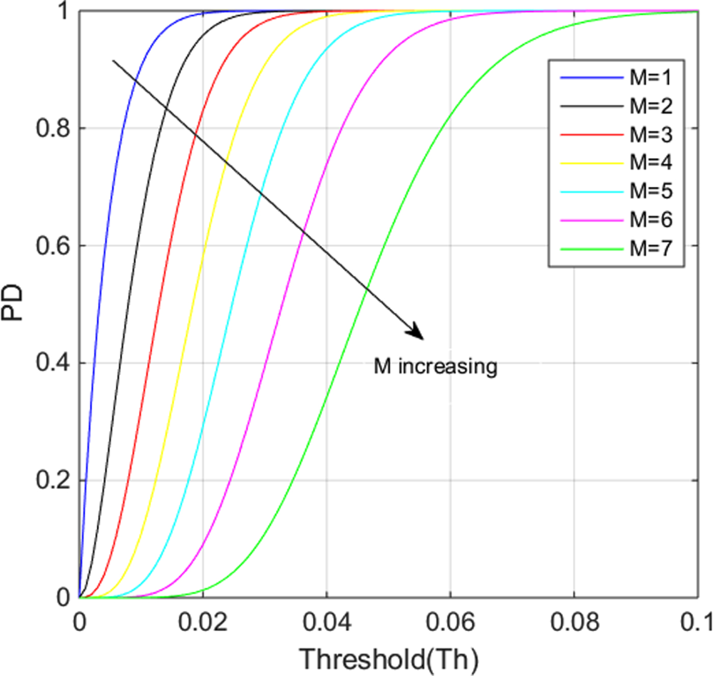
Figure 11. Probability of detection for different M.

Figure 12. Probability of false alarm for different M.

Figure 13. ROC curves of pairwise check connecting (P FA, P D) pairs.
5. EXPERIMENTS
To verify the proposed method, two experiments under two conditions—spoofing conditions and authentic conditions, were carried out. From the published literature, it is not easy to obtain complete equipment for spoofing and anti-spoofing experiments especially in the domestic arena and it is illegal to spread spoofing signals outdoors. Therefore, the experiment under spoofing conditions was carried out using a GNSS signal transponder (THC-TRANS-GB series) which can bring outdoor GNSS satellite signals indoors. In general, all the retransmitting GNSS signals are from the same indoor transmitting antenna of the GNSS signal transponder, which means all GNSS PRNs have the same propagation path.
In the experiments, we employed two Hi-Target V8 GNSS receivers working in Global Positioning System (GPS) L1C mode. The elevation masks for satellites were set at 15° and the sample interval of carrier phase observations was set as 5 seconds. The distance between the two receivers was about 50 cm. The two receivers can automatically record and save original observation data, which we copied to the PC for follow-up processing.
5.1. Experiment in the non-spoofed case
The experiment time was 10:14–10:44 on 9 February 2018. We put the two receivers on a high iron frame located at the roof of No. 113 building of College of Electrical Engineering, Naval University of Engineering, as shown in Figure 14.

Figure 14. Experiment scene in the non-spoofed case.
Through post-processing of the static data, the distribution of available GPS satellites in the non-spoofed case was obtained, as shown in Figures 15 and 16. We found that over 30 minutes, there were eight satellites (PRN 2, PRN 5, PRN 13, PRN 15, PRN 20, PRN 21, PRN 24 and PRN 29) which were always available.

Figure 15. Visibility of GPS satellites in the non-spoofed case.

Figure 16. Number of available GPS satellites in the non-spoofed case.
The seven groups of the double-difference carrier phase observations can be obtained based on the carrier phase observations of the eight available satellites. By normalisation, ϕBAij can be obtained as shown in Figure 17. When the threshold is fixed at T h=0·106 cycles, the test parameter sp can be obtained as shown in Figure 18.
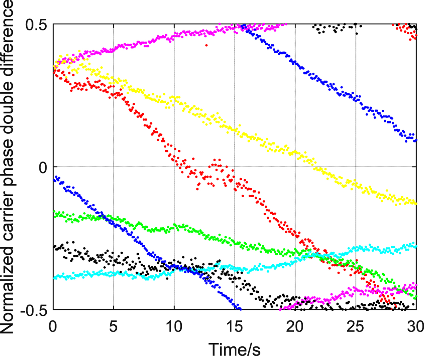
Figure 17. Variation tendency of φBAij in the non-spoofed case.

Figure 18. Variation tendency of Sp in the non-spoofed case.
As shown in Figure 17, the normalised carrier differences in the non-spoofed case change considerably between −0·5~0·5. Taking the blue curve as an example, when the normalised carrier differences are around the −0·5 or 0·5 values, a constant phase cycle slip appears among the adjacent values. That is consistent with theoretical analysis based on Equation (6): −3·49, −3·51−>−0·49, 0·49. As shown in Figure 18, all the values of sp are not more than 2, which means as the threshold of sp is set as 3~7, there will be no false alarms for the spoofing detection unit, in the non-spoofed case.
5.2. Experiment in the spoofed case
Experiment Time was 10:14–10:44 on 10 February 2018. The outdoor antenna of the GNSS signal transponder was placed on the high iron frame located at the roof of No. 113 building of College of Electrical Engineering and the indoor antenna of GNSS signal transponder was placed in the corner of the laboratory, as shown in Figure 19.

Figure 19. Experiment scene in the spoofed case.
Through post-processing of the static data, the distribution of available GPS satellites in the spoofed case is exactly the same as that in the non-spoofed case, since the motion period of GPS satellites is about 24 hours.
The seven groups of the double-difference carrier phase observations can be obtained based on the carrier phase observations of the eight available satellites. After normalisation, can be obtained as shown in Figure 20. When the threshold is fixed at =0·106 cycles, the test parameter sp can be obtained as shown in Figure 21.

Figure 20. Variation tendency of ϕBAij in the spoofed case.

Figure 21. Variation tendency of Sp in the spoofed case.
As shown in Figure 20, the normalised carrier differences in the spoofed case fluctuate slightly between −0·05~0·05. As is shown in Figure 21, all the values of sp are 7, which means as the threshold of sp is set as 7, the spoofing detection can effectively alert the user to the spoofing attacks.
6. SUMMARY
This paper has presented a GNSS spoofing detection method using fraction parts of double-difference carrier phases. The detection system is based on a two-antenna architecture, which does not need to change the internal hardware structure of the two GNSS receivers. This detection unit can take the form of a software module and can be integrated into one of the two GNSS receivers, or as an independent software module which can run well on a PC or other platforms. The detection algorithm of the spoofing detection system is highly reliable and also relatively simple. It can effectively cope with spoofing attacks with all spoofing signals from the same spoofing transmitting antenna quite well, without the need to know the baseline vector of the two antennae, the directions of authentic signals and the location of the spoofing transmitting antenna. Because of the problem of integer ambiguity, it is quite difficult to calculate the real carrier phases of the signal accurately. The fraction parts of double-difference carrier phases can be obtained by normalisation, and so it is not necessary to calculate the integer ambiguity values. In the decision scheme, the M of N algorithm involving all of the (N−1)-set of fraction parts of double-difference carrier phases, can function well in detecting the spoofing.
To improve the robustness of this method, it is important to take T h and M into account. The use of multi-calendar metadata to make decision and analysis is also worthy of study.
In summary, the spoofing detection system described in this paper is easy to apply to a GNSS anti-spoofing receiver, with simple and effective characteristics. However, further developments are needed in order to produce a sufficiently reliable detection system for other spoofing scenarios.
ACKNOWLEDGMENT
This paper is supported by the Natural Science Foundation of China (Nos. 41704034, 41674037, 41631072).


