


INTRODUCTION
Natural and anthropogenic carbon sources and sinks affect the radiocarbon concentration in the atmosphere at the same time. These effects affect the 14C/12C ratio both at a local and global scale (Graven et al. Reference Graven2015; Major et al. Reference Major, Haszpra, Rinyu, Futó, Bihari, Hammer and Molnár2018). The main anthropogenic sources are radiocarbon production from nuclear reactions, such as nuclear weapons testing and the nuclear energy industry. Nuclear bomb tests doubled the natural 14C level in the atmosphere from the late 1950s to early 1960s (Nydal and Lövseth Reference Nydal and Lövseth1983; Buzinny Reference Buzinny2006). This radiocarbon level (known as the “bomb spike”) is decreasing and now is close to the natural, preindustrial or pre-bomb level due to exchange between the terrestrial and oceanic reservoirs and the dilution effect of the addition of fossil-fuel carbon to the atmosphere. The second anthropogenic source is the burning of fossil fuels producing radiocarbon-free greenhouse gases, such as CO2 (Suess Reference Suess1955). These fossil fuels and materials do not contain radiocarbon due to the 5700 ± 30 yr half-life of 14C and long-term geological storage (Bella et al. Reference Bella, Alessio and Fratelli1968; Levin et al. Reference Levin, Naegler, Kromer, Diehl, Francey, Gomez-Pelaez, Steele, Wagenbach, Weller and Worthy2010; Berhanu et al. Reference Berhanu, Szidat, Brunner, Satar, Schanda, Nyfeler, Battaglia, Steinbacher, Hammer and Leuenberger2017; Varga et al. Reference Varga, Major, Janovics, Kurucz, Veres, Jull, Péter and Molnár2018). The natural sources of radiocarbon are the production of 14C in the troposphere by the 14N(n,p)14C reaction (McNeely Reference McNeely1994; Povinec et al. Reference Povinec, Kwong, Kaizer, Molnár, Nies, Palcsu, Papp, Pham and Jean-Baptise2017) due to cosmic radiation and intensive cosmic events. There are other natural sources that do not cause the enrichment of radiocarbon but can dilute the radiocarbon concentration, such as magmatic or volcanic sources that emit radiocarbon-free carbon to the atmosphere (Shore and Cook Reference Shore and Cook1995; Cook et al. Reference Cook, Hainswort, Sorey, Evans and Southon2001). Plants fix the CO2 from the atmosphere by photosynthesis, so plant materials, such as leaves and tree rings, can be a method of biomonitoring the atmospheric radiocarbon concentration (Pawelczyk and Pazdur Reference Pawelczyk and Pazdur2004; Pazdur et al. Reference Pazdur, Nakamura, Pawelczyk, Pawlyta, Piotrowska, Rakowski, Sensula and Szczepanek2007; Quarta et al. Reference Quarta, Rizzo, D’elia and Calcagnile2007; Rakowski Reference Rakowski2011; Janovics et al. Reference Janovics, Kern, Güttler, Wacker, Barnabás and Molnár2013, Reference Janovics, Kelemen, Kern, Kapitány, Veres, Jull and Molnár2016). Evergreen species are often avoided for this reason but in the tropical regions deciduous trees are less common, so in this study, only evergreen leaf samples were collected as a biological record of atmospheric radiocarbon concentration (Alessio et al. Reference Alessio, Anselmi, Conforto, Improta, Manes and Manfra2002). Samples were collected at 13 sampling points in Bali, Indonesia, close to urban activity and traffic, and far from roads and intensive industry. The samples were prepared and measured by MICADAS type accelerator mass spectrometer (AMS) at the Hertelendi Laboratory of Environmental Studies (HEKAL), Hungary, Debrecen (Synal et al. Reference Synal, Stocker and Suter2007; Molnár et al. Reference Molnár, Janovics, Major, Orsovszki, Gönczi, Veres, Leonard, Castle, Lange, Wacker, Hajdas and Jull2013). The primary aim of the study was to give an overview of the radiocarbon distribution of Bali island and supplement the incomplete radiocarbon information about this region.
METHODS
Sampling Sites
Bali island is part of Indonesia, located east of Java. The population of Bali province is more than four million people. The provincial capital and most populated city is Denpasar. The island is the most popular tourist destination in Indonesia and tourism is the leading contributor to economy (Rahayu et al. Reference Rahayu, Haigh and Amaratunga2018). The climate of the island has typical Asian-Australian monsoon seasonality with dry and wet seasons (Fukumoto et al. Reference Fukumoto, Li, Yasuda, Okamura, Yamada and Kashima2015). The vegetation is mainly evergreen due to the tropical climate. The location of Bali Island is shown in Figure 1. During the sampling campaign, in total, samples of woody plants (tree) leaves were collected at 13 sampling points around the Bali Island (Table 1). The samples, fresh leaves from the end of the branches were collected from different districts, forested areas, rice paddies, and urban vegetation close to busy crossroads as well as urban background areas. A minimum 3 pieces of tree leaves were collected from 180 cm high to determine the local fossil carbon load. Taxon names are listed based on the International Plant Name Index (IPNI 2019).
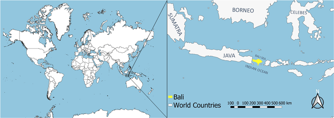
Figure 1 Location of Bali Island.
Table 1 Sampling location and species of plant samples.

SAMPLE PREPARATION AND MEASUREMENT
The collected plant materials were kept frozen until chemical preparation. The samples were cut into small pieces, then homogenized before pretreatment. The standard acid-base-acid preparation protocol was used for the purification of the samples (Southon and Magana Reference Southon and Magana2010), subsequently, the samples were dried in a heating block at 50ºC. The dried samples were combusted in sealed glass tubes at 550ºC for 12 hr, using MnO2 as an oxidant to convert the carbon of organic material to CO2 (Janovics et al. Reference Janovics, Futó and Molnár2018). The liberated CO2 gas was purified from H2O and different contaminants in a dedicated vacuum line. The pure CO2 gas was trapped in glass tubes (with Zn, TiH catalysts and iron powder) sealed by flame and converted to graphite following the sealed tube graphitization method (Rinyu et al. Reference Rinyu, Molnár, Major, Nagy, Veres, Kimák, Wacker and Synal2013). After graphitization, the graphite samples were pressed into aluminium targets for the accelerator mass spectrometry (AMS) measurements to determine the carbon isotopic composition of the plant samples (Molnár et al. Reference Molnár, Janovics, Major, Orsovszki, Gönczi, Veres, Leonard, Castle, Lange, Wacker, Hajdas and Jull2013). For data evaluation, “Bats” data reduction software was used (Wacker et al. Reference Wacker, Christl and Synal2010). For the reporting of 14C data, pMC and Δ14C units were used (Stuiver and Polach Reference Stuiver and Polach1977; Stenström et al. Reference Stenström, Skog, Georgiadou, Grenberg and Johansson2011).
For the environmental samples we use Δ14C units:
 $${\Delta ^{14}}C = \left( {{{{A_{SN}}} \over {{A_{ABS}}}} - 1} \right)\,\,\,\,1000\,{\raise0.5ex\hbox{$\scriptstyle 0$}\kern-0.1em/\kern-0.15em\lower0.25ex\hbox{$\scriptstyle {00}$}}\,\,\,\,\,\,\,\left( {{\rm{without \;age \;correction}}} \right)$$
Where ASN is the stable isotope normalized specific radiocarbon activity of the samples, and AABS is the specific activity of the absolute radiocarbon standard (226 Bq/kg carbon) (Stenström et al. Reference Stenström, Skog, Georgiadou, Grenberg and Johansson2011).
Fossil Contribution
For all the measured samples, the fossil-fuel-derived CO2 ratio (F) and fossil fuel CO2 component (CO2ff) was calculated by the following equations (Levin et al. Reference Levin, Kromer, Schmidt and Sartorius2003):
 $$ F = {{{\Delta ^{14}}{C_{bg}} - {\Delta ^{14}}{C_{meas}}} \over {{\Delta ^{14}}{C_{bg}} + 1000}\,{\raise0.5ex\hbox{$\scriptstyle 0$}\kern-0.1em/\kern-0.15em\lower0.25ex\hbox{$\scriptstyle {00}$}}} $$
Where Δ14Cbg is the radiocarbon content of the background sample, Δ14Cmeas is the radiocarbon content of the measured sample (Baydoun et al. Reference Baydoun, Samad, Nsouli and Younes2015). In our case, the Δ14Cbg is represented by the sample with the highest measured radiocarbon content, due to the lack of proper local background atmospheric 14CO2 measurements, the highest Δ14C value represents the lowest fossil carbon content.
 $$ C{O_{2ff}}\left( {ppmv} \right)\,\, = \,\,{{C{O_{2meas}}\left( {{\Delta ^{14}}{C_{bg}} - {\Delta ^{14}}{C_{meas}}} \right)} \over {{\Delta ^{14}}{C_{bg}} + 1000}\,{\raise0.5ex\hbox{$\scriptstyle 0$}\kern-0.1em/\kern-0.15em\lower0.25ex\hbox{$\scriptstyle {00}$}}} $$
Where Δ14Cbg is the radiocarbon content of the background sample, Δ14Cmeas is the radiocarbon content of the measured sample, CO2meas is the measured CO2 content in the atmosphere at the time of sampling (Berhanu et al. Reference Berhanu, Szidat, Brunner, Satar, Schanda, Nyfeler, Battaglia, Steinbacher, Hammer and Leuenberger2017). In this study, the CO2meas is represented by the annual CO2 concentration (ppm) in 2018 at Mauna Loa, Hawaii, 408.5 ppm (NOAA 2019).
Based on these calculations, the fossil carbon contribution can be estimated in the air and indirectly in the vegetation.
RESULTS AND DISCUSSION
The differentiation of the Δ14C data of evergreen plant samples is not simple, because the growing season is not as well-defined, as the case of deciduous species. Due to this situation, the comparison to atmospheric 14CO2 data is not the same for every sample, because some leaves may have created at different time and the evergreen leaves may store fixed carbon from previous years (Pataki et al. Reference Pataki, Randerson, Wang, Herzenach, Grulke, West, Bowen, Dawson and Tu2010). For this reason, we compared our results to each other and the local “background” to identify the most radiocarbon depleted areas. Table 2 lists the results of AMS measurements of plant samples. The highest Δ14C data, equal to or greater than 11.8‰ were measured at the sampling point no. 3, 6, and 11. These sampling points were at rice fields (no. 3 and 6) and an urban background area on the southern coast (no. 11). These areas were relatively distant from direct urban CO2 emissions and industrial facilities, a minimum 100 m away from roads. Although the longevity of evergreen leaves can be more than one year (Ewers and Schmid Reference Ewers and Schmid1981), in our case, only fresh leaves were collected.
Table 2 Summary of 14C results taken at different sampling districts of Bali, Indonesia.

* The sample with the highest measured radiocarbon content (Δ14Cbg).
The average Δ14C value is 2.2‰ but the scatter is ± 19‰ in case of 13 sampling point. There are two higher values, which are samples taken from urban districts, close to busy crossroads with heavy traffic at sampling points no. 9 and 10. Furthermore, there are two relatively lower Δ14C data at sampling points no. 4 and 13 from different parking places of a tourist attraction and the airport of Denpasar. The most polluted area was a crossroad (no. 10) where the traffic is moderated by a traffic light with a long waiting time for cars and scooters. This has the result that vehicles’ idling engines emit radiocarbon-free CO2 in high concentration continuously at this point source. In this approach, the crossroads can be identified as local point sources of fossil-fuel derived CO2. The second most polluted area is a crossroad as well, at the end of the motorway, a six-lane road, where the conditions are similar to the no. 9 sampling point. These areas are well shielded by buildings and concrete fences, which can regulate the mixing of the air by local winds. The urban background samples and materials from rice fields show generally higher than 5‰ Δ14C data (from 7.5 ± 4.6‰ to 18.2 ± 4.6‰). The 13 Δ14C data points show that the radiocarbon concentration of air in most parts of Bali island is not so depleted.
The spatial distribution is given in Figure 2 and shows that the most depleted area is the densely populated southern region where local urban and tourist activity causes heavy traffic. The radiocarbon-free CO2, mainly due to vehicular traffic, can dilute the local radiocarbon concentration in the frequented area. These data show that the Suess effect is observable on a local scale in a less industrialized region such as Bali as well. Close to Mount Batur, in a volcanic caldera (sampling point no. 4) there is no clearly observable radiocarbon depletion, the relatively lower Δ14C data (0.9 ± 4.5‰) is presumably a consequence of the effect of tourist traffic in the nearby parking places, but cannot be clearly attributed as volcanic or magmatic CO2 emission. Our data shows that the Δ14C level is a little higher than zero ‰ in this equatorial, tropical region. It seems the declining radiocarbon bomb-peak is close to the preindustrial level. The fossil-fuel contribution to the local environment varies between 0.3 and 25.8 ppmv compared to the local background sample (Figure 3).

Figure 2 Map of the Δ14C results in Bali, Indonesia.

Figure 3 Fossil-fuel component (CO2ff) using radiocarbon concentration in leaf samples. The transparent gray bar with dashed line indicates the error of the CO2ff calculation.
As shown by the Δ14C data, sampling sites no. 9 and 10 are the most fossil-carbon loaded regions. These sites have dense traffic every day all year long, which causes high local fossil fuel originated CO2 emission by fuel burning and exhaust. The other 10 samples show that the rest of the island is less affected by fossil carbon, with an average CO2ff is 6.4 ± 7.5 ppmv.
CONCLUSION
In this study, evergreen woody plant samples were successfully used to detect a local Suess effect in Bali, Indonesia. There was a clear radiocarbon depletion in urban vegetation, in two cases where the radiocarbon-free CO2 emission sources are the vehicles. At these crowded crossroads in a densely populated area, the local Δ14C levels in the vegetation sampled were –28.2 ± 4.4‰ and –46 ± 4.3‰, compared to the highest data from a rice field, 18.2 ± 4.6‰. The spatial distribution shows that the radiocarbon level in the coastal area is not depleted and the Suess effect is observed only at the urbanized part of the island in densely populated areas. Our data shows that the CO2 concentration in densely populated areas can be 25 ppm more than annual global average CO2 concentration, and the contribution of fossil sources can be 6% in the urban vegetation. Our data is comparable with other studies; the highest fossil contribution in this study is close to the winter seasonal value, 27.2 ppmv published in Kuc and Zimnoch Reference Kuc and Zimnoch1998 (in Krakow). The recent dataset does not contain unusually high fossil carbon contributions, and there are higher measured data in a published study by Pawelczyk and Pazdur (Reference Pawelczyk and Pazdur2004), where the fossil contribution can be higher than 30 ppmv (in Krakow as well). In Quarta et al. (Reference Quarta, Rizzo, D’elia and Calcagnile2007), the highest fossil carbon fraction is only 2.6% while our highest value is 6.3%. In our former study (Varga et al. Reference Varga, Barnucz, Major, Lisztes-Szabó, Jull, László, Pénzes and Molnár2019) the highest measured fossil carbon content was little higher, 9.6%, in a frequent urban area, at a busy crossroad in a Hungarian city, Debrecen. Our study shows that the radiocarbon level in vegetation, which reflects the atmospheric 14CO2 concentration with a good approximation, is approaching the preindustrial level.
ACKOWLEDGMENTS
The research was supported by the European Union and the State of Hungary, co-謹nanced by the European Regional Development Fund in the project of GINOP-2.3.2-15-2016-00009 “ICER”.


