


1 Introduction
Since patterned paper was suggested as a platform for low-cost, portable, and technically simple bioassays (Martinez et al. Reference Martinez, Phillips, Butte and Whitesides2007), extensive research on microfluidic paper-based analytical devices ( $\unicode[STIX]{x1D707}$PAD) has opened the door to a wide range of applications for point-of-care diagnostics (Böhm et al. Reference Böhm, Carstens, Trieb, Schabel and Biesalski2014; Hu et al. Reference Hu, Wang, Wang, Li, Pingguan-Murphy, Lu and Xu2014; Ahmed, Bui & Abbas Reference Ahmed, Bui and Abbas2016; Hong, Kwak & Kim Reference Hong, Kwak and Kim2016; Lin et al. Reference Lin, Gritsenko, Feng, Teh, Lu and Xu2016; Xia, Si & Li Reference Xia, Si and Li2016; Cummins et al. Reference Cummins, Chinthapatla, Ligler and Walker2017). Paper substrates of
  $\unicode[STIX]{x1D707}$PAD may preclude the need for external pumps, making them both cheap to produce and easy to use. The growing applications of
  $\unicode[STIX]{x1D707}$PAD include veterinary medicine, environmental monitoring and food safety (Martinez et al. Reference Martinez, Phillips, Whitesides and Carrilho2009; Yetisen, Akram & Lowe Reference Yetisen, Akram and Lowe2013; Cate et al. Reference Cate, Adkins, Mettakoonpitak and Henry2014).
Paper is composed of a network of cellulose fibres. When paper comes into contact with liquid, pores between the fibres imbibe the liquid by capillary force. Liquid flow through porous media is generally described by Darcy’s law, which relates the flow rate to applied pressure, material permeability and liquid viscosity (Darcy Reference Darcy1856). Washburn (Reference Washburn1921) developed an equation to describe the capillary-driven flow through a cylindrical tube, where the imbibition length is given by  $l=(\unicode[STIX]{x1D70E}R\cos \unicode[STIX]{x1D703}t/(2\unicode[STIX]{x1D707}))^{1/2}$, where
  $\unicode[STIX]{x1D70E}$ is the surface tension,
  $\unicode[STIX]{x1D703}$ is the contact angle,
  $R$ is the tube radius,
  $t$ is the time and
  $\unicode[STIX]{x1D707}$ is the liquid viscosity. Capillary flow through porous media can be assumed to be equivalent to liquid penetration through multiple parallel arranged cylindrical tubes, so that the penetration length can be expressed as
  $l=k\sqrt{t}$, where
  $k$ is a constant proportional to
  $(\unicode[STIX]{x1D70E}R\cos \unicode[STIX]{x1D703}/\unicode[STIX]{x1D707})^{1/2}$. One can predict the imbibition length using the Washburn equation by experimentally measuring
  $k$.
$k$.
Despite its success describing capillary flows in various porous media, the Washburn equation is often not sufficiently accurate when predicting the imbibition length with respect to time on  $\unicode[STIX]{x1D707}$PAD that require precise flow control (Schuchardt & Berg Reference Schuchardt and Berg1991; Amaral et al. Reference Amaral, Barabási, Buldyrev, Havlin and Stanley1994; Bico & Quéré Reference Bico and Quéré2003; Alava & Niskanen Reference Alava and Niskanen2006; Masoodi & Pillai Reference Masoodi and Pillai2010; Balankin et al. Reference Balankin, López, León, Matamoros, Ruiz, López and Rodríguez2013). Our recent study (Chang et al. Reference Chang, Seo, Hong, Lee and Kim2018) demonstrated that flow through internal pores present in the cellulose fibres is one of the central reasons. The experimental tests with silicone oils quantified how the flow through the intra-fibre pores delays the imbibition speed relative to the speed predicted by the Washburn equation. Taking into account the flow through intra-fibre pores, we developed a mathematical model that improves flow speed prediction (MacDonald Reference MacDonald2018). Nevertheless, the model’s application is limited to non-aqueous liquids such as silicone oils which do not cause paper swelling.
Aqueous liquid flow through paper involves paper swelling. The hydroxyl groups in cellulose fibre (-COOH) combine with water molecules, leading to expansion of the cellulose fibre network (Enderby Reference Enderby1955; Topgaard & Söderman Reference Topgaard and Söderman2001; Lee et al. Reference Lee, Kim, Kim and Mahadevan2016). This water absorption thus changes the pore structure of the paper on which the imbibition dynamics depend (Alava & Niskanen Reference Alava and Niskanen2006; Reyssat & Mahadevan Reference Reyssat and Mahadevan2011; Lee et al. Reference Lee, Kim, Kim and Mahadevan2016; Kvick et al. Reference Kvick, Martinez, Hewitt and Balmforth2017). A great deal of effort has been devoted to the theoretical analysis of two-phase flows through a deformable porous medium, but the previous studies mainly focused on the complex interaction between the liquid and porous medium (Preziosi, Joseph & Beavers Reference Preziosi, Joseph and Beavers1996; Sommer & Mortensen Reference Sommer and Mortensen1996; Anderson Reference Anderson2005; Siddique, Anderson & Bondarev Reference Siddique, Anderson and Bondarev2009; Kvick et al. Reference Kvick, Martinez, Hewitt and Balmforth2017). Pillai (Reference Pillai2014) presented a comprehensive theoretical framework to describe the velocity field inside a generalized porous material involving swelling, and discussed the application of the model to liquid imbibition through paper. Although Schuchardt & Berg (Reference Schuchardt and Berg1991) and Masoodi & Pillai (Reference Masoodi and Pillai2010) studied the effect of swelling on liquid imbibition through paper, they used special paper, made by adding superabsorbent material to normal paper, to maximize the swelling effect. Our physical understanding of water imbibition through paper is still unclear, because it does not yet include the swelling effect appropriately.

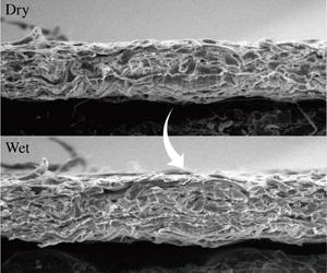
Figure 1. Environmental scanning electron microscope images of the cross-sections of Whatman filter paper (grade 6) in the (a) dry and (b) wet conditions.
Here, we elucidate the role of paper swelling in the dynamics of water imbibition through paper. We visualize the swelling of various filter papers and demonstrate that the expansion of the inter-fibre pores is responsible for the paper swelling. By introducing physical parameters that characterize paper swelling, we propose a mathematical model for the dynamics of water imbibition through paper with swelling. When combined with experimental measurements of paper swelling, rather than complicated polymer physics, the model enables us to accurately predict the flow speed of water through paper, and provides a better physical understanding. Given the various applications of  $\unicode[STIX]{x1D707}$PAD using aqueous liquids, the present study will help us to design
  $\unicode[STIX]{x1D707}$PAD with improved flow control. The theoretical framework of the present study can be extended to capillary flow through various deformable porous media.

Figure 2. Thickness change of various Whatman filter papers of (a) grade 1, (b) grade 4, (c) grade 5 and (d) grade 6, before and after wetting.
2 Experiments
We visualized the swelling of various commercial filter papers (Whatman grade 1, 4, 5 and 6) that absorbed water. The properties of the distilled water used in the experiments are listed in table 1. Figure 1 shows environmental scanning electron microscope images of the cross-section of a filter paper specimen (Whatman grade 6) in dry and wet conditions. In the wet state, a relatively large void fraction was observed between the fibres, and the inter-connections appeared loose. Wet pulp is dried and pressed to produce paper sheets in the papermaking process. In the dry state the cellulose fibre network in the paper sheet remains compressed in the thickness direction (Bajpai Reference Bajpai and Bajpai2015). Contact with water loosens the inter-connections between the fibres, leading to the thickness expansion. The swelling of paper in the in-plane direction was observed to be negligible compared to that in the thickness direction, as reported in other studies (Lee et al. Reference Lee, Kim, Kim and Mahadevan2016; Kvick et al. Reference Kvick, Martinez, Hewitt and Balmforth2017).
Table 1. Properties of liquids used in the experiments: density ( $\unicode[STIX]{x1D70C}$), viscosity (
 $\unicode[STIX]{x1D707}$) and surface tension (
 $\unicode[STIX]{x1D70E}$).

Changes in the average thickness of paper before and after wetting were quantified using optical microscope images of the cross-sections of the filter paper, as shown in figure 2. The thickness change was measured after the paper had fully swelled. We assessed the expansion ratio  $(d_{2}-d_{1})/d_{1}$ using the thicknesses of the dry paper
  $d_{1}$ and wet paper
  $d_{2}$. The time it takes for swelling to complete,
  $t_{s}$, was measured by observing the change in thickness over time after the wetting front passed.
We constructed an experimental set-up to visualize water flow through paper, as shown in figure 3(a). A rectangular paper strip with a width of 5 mm was placed on a horizontal support to preclude gravitational effects on the liquid flow. The paper is known to be anisotropic in two directions on the plane: the machine direction (MD) parallel to the forming direction and the cross-machine direction (CD) perpendicular to the MD (Walji & MacDonald Reference Walji and MacDonald2016). In our experiments, the paper strips were placed so that the water could flow in the MD. We started the imbibition by adjusting the horizontal position of the water reservoir so that an end of the paper strip came into contact with the water. The wetting of each paper strip was observed for ∼60 s at a relative humidity of 40 ± 5 %. The water evaporation rate from a paper surface is approximately 0.05 g (m-2 s-1) at a relative humidity of 40 % (Jahanshahi-Anbuhi et al. Reference Jahanshahi-Anbuhi, Henry, Leung, Sicard, Pennings, Pelton, Brennan and Filipe2014), so that the ratio of water evaporated from the surface of the paper substrate to water absorbed in the paper for ∼60 s is less than 1 %. The wetting front was filmed using a high-speed camera (Photron Mini AX200) while illuminated with LED lights from the top. Figure 3(b) shows sequential images of the wetting front of infiltrating water.

Figure 3. (a) Schematic illustration of the experimental set-up. (b) Sequential images of the paper strip (Whatman grade 5) showing water imbibition. The wet region appears dark, and the boundary between the dark and bright regions indicates the wetting front.
We measured the properties of the pore structure in the paper using imbibition tests with a silicone oil with the properties listed in table 1. The silicone oil tests enabled us to exclude swelling effects. Based on measurements of the time dependence of the mass of the silicone oil absorbed in 5 mm strips of the filter papers, shown in figure 4, we estimated the volume ratio of intra- to inter-fibre pores  $\unicode[STIX]{x1D713}$ and the time it takes the liquid to fill the intra-fibre pores
  $t_{c(o)}$, where the subscript ‘
 $o$’ denotes the properties for silicone oil. We also obtained the proportional constant of the Washburn equation
  $k_{(o)}$ from the observation of the imbibition in the early stages for
  $t<0.1t_{c(o)}$. The details of the silicone oil tests were described in our previous study (Chang et al. Reference Chang, Seo, Hong, Lee and Kim2018).

Figure 4. The time dependence of the mass of the silicone oil absorbed in 5 mm strips of various Whatman filter papers of (a) grade 1, (b) grade 4, (c) grade 5 and (d) grade 6. The mass is scaled as the maximum absorption mass. The star symbols indicate the moment when the liquid front reaches the strip end, and the circle symbols indicate the moment when the mass attains 95 % of its maximum.
We describe the technique to estimate  $k_{(w)}$ and
  $t_{c(w)}$. The subscript ‘
 $w$’ denotes the properties for water. Since water absorption by paper necessarily involves paper swelling, it is impossible to measure the proportional constant for water
  $k_{(w)}$ in the Washburn equation, which neglects intra-fibre pores and swelling, using the technique of measuring
  $k_{(o)}$. Noting that
  $k$ is proportional to
  $(\unicode[STIX]{x1D70E}\cos \unicode[STIX]{x1D703}/\unicode[STIX]{x1D707})^{1/2}$, one can alternatively estimate
  $k_{(w)}=k_{(o)}(\unicode[STIX]{x1D70E}_{(w)}\cos \unicode[STIX]{x1D703}_{(w)}/\unicode[STIX]{x1D707}_{(w)})^{1/2}(\unicode[STIX]{x1D70E}_{(o)}\cos \unicode[STIX]{x1D703}_{(o)}/\unicode[STIX]{x1D707}_{(o)})^{-1/2}$. The flow speed of water is significantly faster than that of silicone oil, so that the technique that we use to measure
  $t_{c(o)}$ for silicone oil cannot be applied to measure
  $t_{c(w)}$ for water. However, it can be estimated as
  $t_{c(w)}=t_{c(o)}(\unicode[STIX]{x1D707}_{(w)}/\unicode[STIX]{x1D70E}_{(w)}\cos \unicode[STIX]{x1D703}_{(w)})(\unicode[STIX]{x1D707}_{(o)}/\unicode[STIX]{x1D70E}_{(o)}\cos \unicode[STIX]{x1D703}_{(o)})^{-1}$ because
  $t_{c}$ is proportional to
  $\unicode[STIX]{x1D707}/(\unicode[STIX]{x1D70E}\cos \unicode[STIX]{x1D703})$ for a specific paper (Chang et al. Reference Chang, Seo, Hong, Lee and Kim2018). The ratio of the contact angles of two liquids in a porous medium can be assessed from the Jurin height (Jurin Reference Jurin1718). A vertically suspended paper absorbs liquid up to a height where the hydrostatic pressure balances the Laplace pressure, and the rise height is proportional to
  $\unicode[STIX]{x1D70E}\cos \unicode[STIX]{x1D703}/(\unicode[STIX]{x1D70C}gR)$, where
  $\unicode[STIX]{x1D70C}$ is the liquid density, and
  $g$ is the gravitational acceleration (Hong & Kim Reference Hong and Kim2015). We measured the maximum rise height on a filter paper (Whatman grade 4) to be 158 mm for water and 86 mm for silicone oil. Since
  $\unicode[STIX]{x1D70C}_{(w)}/\unicode[STIX]{x1D70C}_{(o)}\approx 1.1$ and
  $\unicode[STIX]{x1D70E}_{(w)}/\unicode[STIX]{x1D70E}_{(o)}\approx 3.6$, we deduced
  $\cos \unicode[STIX]{x1D703}_{(w)}/\cos \unicode[STIX]{x1D703}_{(o)}\approx 0.53$. Combining these data with
  $\unicode[STIX]{x1D707}_{(w)}/\unicode[STIX]{x1D707}_{(o)}\approx 0.2$ yielded
  $k_{(w)}/k_{(o)}\approx 3.1$ and
  $t_{c(w)}/t_{c(o)}\approx 0.1$, and
  $k_{(w)}$ and
  $t_{c(w)}$ were finally obtained. The assessed various physical properties of the filter papers are listed in table 2.
Table 2. Properties of various Whatman filter papers used in the experiments.


Figure 5. The capillary tube geometries for (a) the Washburn equation, (b) the model that considers only intra-fibre pores, and (c) the present model that considers swelling and intra-fibre pores.
3 Theoretical analysis
We start the theoretical analysis by constructing a geometric model which includes the swelling of inter-fibre pores as well as the absorption of intra-fibre pores, as shown in figure 5. The cylindrical tube shown in figure 5(a) was employed to develop the Washburn equation. In our previous study a rigid cylindrical tube with an additional slit, shown in figure 5(b), was used to consider the intra-fibre pores (Chang et al. Reference Chang, Seo, Hong, Lee and Kim2018). The radius of the cylindrical tube  $R$ is equivalent to the average radius of the inter-fibre pores of the paper in a dry state, and the gap,
  $e$, in the slit is the average diameter of the intra-fibre pores. The slit height
  $H$ determines the volume of the intra-fibre pores, and the volume ratio of the intra- to inter-fibre pores is given by
  $\unicode[STIX]{x1D713}=eH/\unicode[STIX]{x03C0}R^{2}$. In contrast, in the present geometric model, the cylindrical tube with a slit can radially expand upon contact with liquid, and as a result the tube radius can vary in the axial direction, as shown in figure 5(c). In addition to the side slit corresponding to the intra-fibre pores, the expandable cylindrical tube allows for the expansion of the inter-fibre pores leading to paper swelling. The tube radius
  $r$ thus depends on the local expansion in inter-fibre pores. The expansion is bounded by the maximum tube radius
  $R+\unicode[STIX]{x0394}R$, which is determined by the volume of swollen paper.
We consider water flow in the slit at a specific time  $t$ when the cylindrical tube imbibes water to a length of
  $l$. The momentum equation in the slit is determined by the balance between the capillary force and viscous resistance, which is expressed as
  $\unicode[STIX]{x1D70E}e\sim \unicode[STIX]{x1D707}hh^{\prime }$, where
  $h$ and
  $h^{\prime }=\text{d}h/\text{d}t$ are the imbibition length and speed in the slit, respectively. At a location separated from the tube inlet by
  $\unicode[STIX]{x1D709}$, the imbibition length in the slit is thus given by
 $$\begin{eqnarray}h(\unicode[STIX]{x1D709})=k_{s}\sqrt{t-\unicode[STIX]{x1D70F}},\quad t\geqslant \unicode[STIX]{x1D70F},\end{eqnarray}$$
 where  $k_{s}$ is the proportional constant,
  $\unicode[STIX]{x1D70F}$ is the time satisfying
  $l(\unicode[STIX]{x1D70F})=\unicode[STIX]{x1D709}$, thus implying that
  $t-\unicode[STIX]{x1D70F}$ is the local suction time through the slit.
We quantify the expansion of the capillary tube. Paper swelling is the result of the deformation of the cellulose fibre network, and the swelling dynamics thus involves complicated polymer physics. Nevertheless, our experimental observations allow us to simply assume that the cylindrical tube expands at a constant speed of  $v_{s}=\unicode[STIX]{x0394}R/t_{s}$ with the swelling time
  $t_{s}$. The swelling time for all the papers that we tested is approximately 3 s, which is sufficiently short compared with the water imbibition time ∼60 s in our experiments, so that the variation in swelling speed within
  $t_{s}$ negligibly affects the imbibition dynamics. We express the local radius of the cylindrical tube as
 $$\begin{eqnarray}r(\unicode[STIX]{x1D709})=R+v_{s}(t-\unicode[STIX]{x1D70F}),\quad t\geqslant \unicode[STIX]{x1D70F}.\end{eqnarray}$$
 The momentum equation in the cylindrical tube is obtained from the balance between the capillary force and the viscous resistance. Because of water flow through the slit and the tube expansion, the flow speed through the cylindrical tube is not constant in the axial direction. The momentum equation is given in an integral form,  $\unicode[STIX]{x1D70E}\cos \unicode[STIX]{x1D703}(2\unicode[STIX]{x03C0}R)=\int _{0}^{l}\unicode[STIX]{x1D6FE}(2\unicode[STIX]{x03C0}r)\,\text{d}\unicode[STIX]{x1D709}$, where
  $\unicode[STIX]{x1D6FE}=4\unicode[STIX]{x1D707}u/r$ is the local shear stress on the inner surface of the cylindrical tube with
  $u$ being the local average flow speed in the tube. By substituting
  $(\unicode[STIX]{x1D70E}R\cos \unicode[STIX]{x1D703}/(2\unicode[STIX]{x1D707}))^{1/2}$ with
  $k$, one can simplify the momentum equation to
 $$\begin{eqnarray}\int _{0}^{l}u\,\text{d}\unicode[STIX]{x1D709}=\frac{1}{2}k^{2}.\end{eqnarray}$$
 The equations (3.1)–(3.3) are coupled via continuity of mass. The continuity equation in differential form is given by  $-\unicode[STIX]{x03C0}r^{2}(\text{d}u/\text{d}\unicode[STIX]{x1D709})=(h^{\prime }-v_{s})e+2\unicode[STIX]{x03C0}v_{s}r$. Here the right-hand side can be reduced to
  $h^{\prime }e+2\unicode[STIX]{x03C0}v_{s}r$. The size of the inter-fibre pores
  $r$ is one order greater than that of intra-fibre pores
  $e$ (Chang et al. Reference Chang, Seo, Hong, Lee and Kim2018), and we thus deduce that
  $h^{\prime }e+(2\unicode[STIX]{x03C0}r-e)v_{s}\sim h^{\prime }e+2\unicode[STIX]{x03C0}v_{s}r$. By integrating the reduced continuity equation from
  $\unicode[STIX]{x1D709}$ to
  $l$, we obtain
 $$\begin{eqnarray}u(\unicode[STIX]{x1D709})=l^{\prime }(t)+\int _{\unicode[STIX]{x1D709}}^{l}\left(\frac{eh^{\prime }}{\unicode[STIX]{x03C0}r^{2}}+\frac{2v_{s}}{r}\right)\text{d}\unicode[STIX]{x1D709},\end{eqnarray}$$
 with  $l^{\prime }$ being
  $\text{d}l/\text{d}t$, since
  $u(l)=l^{\prime }(t)$.
To solve for  $l(t)$, we obtain a single governing equation by substituting (3.4) into (3.3) to give
 $$\begin{eqnarray}l(t)l^{\prime }(t)+\int _{0}^{l}\int _{\unicode[STIX]{x1D709}}^{l}\left(\frac{eh^{\prime }}{\unicode[STIX]{x03C0}r^{2}}+\frac{2v_{s}}{r}\right)\text{d}\unicode[STIX]{x1D709}\,\text{d}\unicode[STIX]{x1D709}=\frac{1}{2}k^{2},\end{eqnarray}$$
 where  $h^{\prime }$,
  $r$ and
  $v_{s}$ are determined by (3.1) and (3.2). Since the solution of (3.5) depends on the relative magnitude between
  $t_{c}$ and
  $t_{s}$, we proceed with the analysis of each case.

Figure 6. Schematics of the phases of water imbibition for the cases of (a)  $t_{c}<t_{s}$ and (b)
  $t_{c}>t_{s}$.
3.1 Case of  $t_{c}<t_{s}$

We first consider the case of  $t_{c}<t_{s}$. Near the channel entrance, water completely fills the slit before the tube expansion ends. The imbibition progress can be divided into three phases, for the times
  $t<t_{c}$,
  $t_{c}<t<t_{s}$ and
  $t>t_{s}$, respectively (see figure 6a). In the first phase for
  $t<t_{c}$, the swelling of the cylindrical tube and the imbibition through the slit occur over the entire tube length in contact with water behind the wetting front. For the time
  $t_{c}<t<t_{s}$, the anterior part of the slit is fully filled and thus does not suck water, while swelling still occurs over the entire tube length in contact with water. For
  $t>t_{s}$, the anterior part of the tube does not have swelling or water flow through the slit.
In the first phase for the time  $t<t_{c}$, we substitute
  $h^{\prime }=k_{s}/(2\sqrt{t-\unicode[STIX]{x1D70F}})$,
  $v_{s}=\unicode[STIX]{x0394}R/t_{s}$ and
  $r=R+\unicode[STIX]{x0394}R(t-\unicode[STIX]{x1D70F})/t_{s}$ in (3.5), leading to
 $$\begin{eqnarray}\displaystyle & & \displaystyle l(t)l^{\prime }(t)+\frac{k_{s}e}{2\unicode[STIX]{x03C0}}\int _{0}^{t}\left(\int _{\unicode[STIX]{x1D70F}}^{t}\frac{l^{\prime }(\unicode[STIX]{x1D70F})}{(R+\unicode[STIX]{x0394}R(t-\unicode[STIX]{x1D70F})/t_{s})^{2}\sqrt{t-\unicode[STIX]{x1D70F}}}\,\text{d}\unicode[STIX]{x1D70F}\right)l^{\prime }(\unicode[STIX]{x1D70F})\,\text{d}\unicode[STIX]{x1D70F}\nonumber\\ \displaystyle & & \displaystyle \quad +\,\frac{2\unicode[STIX]{x0394}R}{t_{s}}\int _{0}^{t}\left(\int _{\unicode[STIX]{x1D70F}}^{t}\frac{l^{\prime }(\unicode[STIX]{x1D70F})}{R+\unicode[STIX]{x0394}R(t-\unicode[STIX]{x1D70F})/t_{s}}\,\text{d}\unicode[STIX]{x1D70F}\right)l^{\prime }(\unicode[STIX]{x1D70F})\,\text{d}\unicode[STIX]{x1D70F}=\frac{1}{2}k^{2},\end{eqnarray}$$
 where  $\text{d}\unicode[STIX]{x1D709}=l^{\prime }(\unicode[STIX]{x1D70F})\,\text{d}\unicode[STIX]{x1D70F}$ is used.
In the second phase for the time  $t_{c}<t<t_{s}$, the expressions of
  $h^{\prime }$,
  $r$ and
  $v_{s}$ are distinct in the regions of
  $0<\unicode[STIX]{x1D709}<\unicode[STIX]{x1D6FC}$ and
  $\unicode[STIX]{x1D709}>\unicode[STIX]{x1D6FC}$, where
  $\unicode[STIX]{x1D6FC}=l(t-t_{c})$ is the length of the slit saturated with water. In the range of
  $0<\unicode[STIX]{x1D709}<\unicode[STIX]{x1D6FC}$,
  $h^{\prime }=0$,
  $v_{s}=\unicode[STIX]{x0394}R/t_{s}$ and
  $r=R+\unicode[STIX]{x0394}R(t-\unicode[STIX]{x1D70F})/t_{s}$. For
  $\unicode[STIX]{x1D709}>\unicode[STIX]{x1D6FC}$,
  $h^{\prime }=k_{s}/(2\sqrt{t-\unicode[STIX]{x1D70F}})$,
  $v_{s}=\unicode[STIX]{x0394}R/t_{s}$ and
  $r=R+\unicode[STIX]{x0394}R(t-\unicode[STIX]{x1D70F})/t_{s}$. Substituting these expressions into (3.5) yields
 $$\begin{eqnarray}\displaystyle & & \displaystyle l(t)l^{\prime }(t)+\frac{k_{s}e}{2\unicode[STIX]{x03C0}}\left\{\int _{0}^{t-t_{c}}\left(\int _{t-t_{c}}^{t}\frac{l^{\prime }(\unicode[STIX]{x1D70F})}{(R+\unicode[STIX]{x0394}R(t-\unicode[STIX]{x1D70F})/t_{s})^{2}\sqrt{t-\unicode[STIX]{x1D70F}}}\,\text{d}\unicode[STIX]{x1D70F}\right)l^{\prime }(\unicode[STIX]{x1D70F})\,\text{d}\unicode[STIX]{x1D70F}\right.\nonumber\\ \displaystyle & & \displaystyle \left.\quad +\,\int _{t-t_{c}}^{t}\left(\int _{\unicode[STIX]{x1D70F}}^{t}\frac{l^{\prime }(\unicode[STIX]{x1D70F})}{(R+\unicode[STIX]{x0394}R(t-\unicode[STIX]{x1D70F})/t_{s})^{2}\sqrt{t-\unicode[STIX]{x1D70F}}}\,\text{d}\unicode[STIX]{x1D70F}\right)l^{\prime }(\unicode[STIX]{x1D70F})\,\text{d}\unicode[STIX]{x1D70F}\right\}\nonumber\\ \displaystyle & & \displaystyle \quad +\,\frac{2\unicode[STIX]{x0394}R}{t_{s}}\int _{0}^{t}\left(\int _{\unicode[STIX]{x1D70F}}^{t}\frac{l^{\prime }(\unicode[STIX]{x1D70F})}{R+\unicode[STIX]{x0394}R(t-\unicode[STIX]{x1D70F})/t_{s}}\,\text{d}\unicode[STIX]{x1D70F}\right)l^{\prime }(\unicode[STIX]{x1D70F})\,\text{d}\unicode[STIX]{x1D70F}=\frac{1}{2}k^{2}.\end{eqnarray}$$
 We consider the last phase for  $t>t_{s}$. The expressions of
  $h^{\prime }$,
  $r$ and
  $v_{s}$ are distinct in three regions of
  $0<\unicode[STIX]{x1D709}<\unicode[STIX]{x1D6FD}$,
  $\unicode[STIX]{x1D6FD}<\unicode[STIX]{x1D709}<\unicode[STIX]{x1D6FC}$ and
  $\unicode[STIX]{x1D709}>\unicode[STIX]{x1D6FC}$, where
  $\unicode[STIX]{x1D6FD}=l(t-t_{s})$ is the length of the fully swollen part of the tube. In the range of
  $0<\unicode[STIX]{x1D709}<\unicode[STIX]{x1D6FD}$,
  $h^{\prime }=0$,
  $v_{s}=0$ and
  $r=R+\unicode[STIX]{x0394}R$. For
  $\unicode[STIX]{x1D6FD}<\unicode[STIX]{x1D709}<\unicode[STIX]{x1D6FC}$,
  $h^{\prime }=0$,
  $v_{s}=\unicode[STIX]{x0394}R/t_{s}$ and
  $r=R+\unicode[STIX]{x0394}R(t-\unicode[STIX]{x1D70F})/t_{s}$. For
  $\unicode[STIX]{x1D709}>\unicode[STIX]{x1D6FC}$,
  $h^{\prime }=k_{s}/(2\sqrt{t-\unicode[STIX]{x1D70F}})$,
  $v_{s}=\unicode[STIX]{x0394}R/t_{s}$ and
  $r=R+\unicode[STIX]{x0394}R(t-\unicode[STIX]{x1D70F})/t_{s}$. By substituting these in (3.5), we obtain
 $$\begin{eqnarray}\displaystyle & & \displaystyle l(t)l^{\prime }(t)+\frac{k_{s}e}{2\unicode[STIX]{x03C0}}\left\{\int _{0}^{t-t_{c}}\left(\int _{t-t_{c}}^{t}\frac{l^{\prime }(\unicode[STIX]{x1D70F})}{(R+\unicode[STIX]{x0394}R(t-\unicode[STIX]{x1D70F})/t_{s})^{2}\sqrt{t-\unicode[STIX]{x1D70F}}}\,\text{d}\unicode[STIX]{x1D70F}\right)l^{\prime }(\unicode[STIX]{x1D70F})\,\text{d}\unicode[STIX]{x1D70F}\right.\nonumber\\ \displaystyle & & \displaystyle \left.\quad +\,\int _{t-t_{c}}^{t}\left(\int _{\unicode[STIX]{x1D70F}}^{t}\frac{l^{\prime }(\unicode[STIX]{x1D70F})}{(R+\unicode[STIX]{x0394}R(t-\unicode[STIX]{x1D70F})/t_{s})^{2}\sqrt{t-\unicode[STIX]{x1D70F}}}\,\text{d}\unicode[STIX]{x1D70F}\right)l^{\prime }(\unicode[STIX]{x1D70F})\,\text{d}\unicode[STIX]{x1D70F}\right\}\nonumber\\ \displaystyle & & \displaystyle \quad +\,\frac{2\unicode[STIX]{x0394}R}{t_{s}}\left\{\int _{0}^{t-t_{s}}\left(\int _{t-t_{s}}^{t}\frac{l^{\prime }(\unicode[STIX]{x1D70F})}{R+\unicode[STIX]{x0394}R(t-\unicode[STIX]{x1D70F})/t_{s}}\,\text{d}\unicode[STIX]{x1D70F}\right)l^{\prime }(\unicode[STIX]{x1D70F})\,\text{d}\unicode[STIX]{x1D70F}\right.\nonumber\\ \displaystyle & & \displaystyle \left.\quad +\,\int _{t-t_{s}}^{t}\left(\int _{\unicode[STIX]{x1D70F}}^{t}\frac{l^{\prime }(\unicode[STIX]{x1D70F})}{R+\unicode[STIX]{x0394}R(t-\unicode[STIX]{x1D70F})/t_{s}}\,\text{d}\unicode[STIX]{x1D70F}\right)l^{\prime }(\unicode[STIX]{x1D70F})\,\text{d}\unicode[STIX]{x1D70F}\right\}=\frac{1}{2}k^{2}.\end{eqnarray}$$
3.2 Case of $t_{c}>t_{s}$

We analyse the case  $t_{c}>t_{s}$ in the same way as in § 3.1. In this case, the tube swelling near the channel entrance first ends before the water suction in the slit is completed. Figure 6(b) displays the schematics of the three imbibition phases for the times
  $t<t_{s}$,
  $t_{s}<t<t_{c}$ and
  $t>t_{c}$, respectively. In the first phase for
  $t<t_{s}$, the swelling of the cylindrical tube and the imbibition through the slit occurs over the entire tube length in contact with water behind the wetting front. For the time
  $t_{s}<t<t_{c}$, the anterior part of the tube is fully swollen, so that the tube radius is
  $R+\unicode[STIX]{x0394}R$, while the entire slit behind the wetting front still sucks water. For
  $t>t_{c}$, the anterior part of the tube does not have swelling or water flow through the slit.
In the first phase for the time  $t<t_{s}$, we replace
  $h^{\prime }=k_{s}/(2\sqrt{t-\unicode[STIX]{x1D70F}})$,
  $v_{s}=\unicode[STIX]{x0394}R/t_{s}$ and
  $r=R+\unicode[STIX]{x0394}R(t-\unicode[STIX]{x1D70F})/t_{s}$ in (3.5), so that the equation for
  $l$ is the same as (3.6).
In the second phase for the time  $t_{s}<t<t_{c}$, the expressions of
  $h^{\prime }$,
  $r$ and
  $v_{s}$ are distinct in the regions
  $0<\unicode[STIX]{x1D709}<\unicode[STIX]{x1D6FD}$ and
  $\unicode[STIX]{x1D709}>\unicode[STIX]{x1D6FD}$. In the range of
  $0<\unicode[STIX]{x1D709}<\unicode[STIX]{x1D6FD}$,
  $h^{\prime }=k_{s}/(2\sqrt{t-\unicode[STIX]{x1D70F}})$,
  $v_{s}=0$ and
  $r=R+\unicode[STIX]{x0394}R$, while
  $h^{\prime }=k_{s}/(2\sqrt{t-\unicode[STIX]{x1D70F}})$,
  $v_{s}=\unicode[STIX]{x0394}R/t_{s}$ and
  $r=R+\unicode[STIX]{x0394}R(t-\unicode[STIX]{x1D70F})/t_{s}$ for
  $\unicode[STIX]{x1D709}>\unicode[STIX]{x1D6FD}$. Substituting these into (3.5) yields
 $$\begin{eqnarray}\displaystyle & & \displaystyle l(t)l^{\prime }(t)+\frac{k_{s}e}{2\unicode[STIX]{x03C0}}\left\{\int _{0}^{t-t_{s}}\left(\int _{\unicode[STIX]{x1D70F}}^{t-t_{s}}\frac{l^{\prime }(\unicode[STIX]{x1D70F})}{(R+\unicode[STIX]{x0394}R)^{2}\sqrt{t-\unicode[STIX]{x1D70F}}}\,\text{d}\unicode[STIX]{x1D70F}\right)l^{\prime }(\unicode[STIX]{x1D70F})\,\text{d}\unicode[STIX]{x1D70F}\right.\nonumber\\ \displaystyle & & \displaystyle \left.\quad +\,\int _{0}^{t-t_{s}}\left(\int _{t-t_{s}}^{t}\frac{l^{\prime }(\unicode[STIX]{x1D70F})}{(R+\unicode[STIX]{x0394}R(t-\unicode[STIX]{x1D70F})/t_{s})^{2}\sqrt{t-\unicode[STIX]{x1D70F}}}\,\text{d}\unicode[STIX]{x1D70F}\right)l^{\prime }(\unicode[STIX]{x1D70F})\,\text{d}\unicode[STIX]{x1D70F}\right.\nonumber\\ \displaystyle & & \displaystyle \left.\quad +\,\int _{t-t_{s}}^{t}\left(\int _{\unicode[STIX]{x1D70F}}^{t}\frac{l^{\prime }(\unicode[STIX]{x1D70F})}{(R+\unicode[STIX]{x0394}R(t-\unicode[STIX]{x1D70F})/t_{s})^{2}\sqrt{t-\unicode[STIX]{x1D70F}}}\,\text{d}\unicode[STIX]{x1D70F}\right)l^{\prime }(\unicode[STIX]{x1D70F})\,\text{d}\unicode[STIX]{x1D70F}\right\}\nonumber\\ \displaystyle & & \displaystyle \quad +\,\frac{2\unicode[STIX]{x0394}R}{t_{s}}\left\{\int _{0}^{t-t_{s}}\left(\int _{t-t_{s}}^{t}\frac{l^{\prime }(\unicode[STIX]{x1D70F})}{R+\unicode[STIX]{x0394}R(t-\unicode[STIX]{x1D70F})/t_{s}}\,\text{d}\unicode[STIX]{x1D70F}\right)l^{\prime }(\unicode[STIX]{x1D70F})\,\text{d}\unicode[STIX]{x1D70F}\right.\nonumber\\ \displaystyle & & \displaystyle \left.\quad +\,\int _{t-t_{s}}^{t}\left(\int _{\unicode[STIX]{x1D70F}}^{t}\frac{l^{\prime }(\unicode[STIX]{x1D70F})}{R+\unicode[STIX]{x0394}R(t-\unicode[STIX]{x1D70F})/t_{s}}\,\text{d}\unicode[STIX]{x1D70F}\right)l^{\prime }(\unicode[STIX]{x1D70F})\,\text{d}\unicode[STIX]{x1D70F}\right\}=\frac{1}{2}k^{2}.\end{eqnarray}$$
 We consider the last phase for  $t>t_{c}$. We consider separately the three regions,
  $0<\unicode[STIX]{x1D709}<\unicode[STIX]{x1D6FC}$,
  $\unicode[STIX]{x1D6FC}<\unicode[STIX]{x1D709}<\unicode[STIX]{x1D6FD}$ and
  $\unicode[STIX]{x1D709}>\unicode[STIX]{x1D6FD}$. In the range of
  $0<\unicode[STIX]{x1D709}<\unicode[STIX]{x1D6FC}$,
  $h^{\prime }=0$,
  $v_{s}=0$ and
  $r=R+\unicode[STIX]{x0394}R$. For
  $\unicode[STIX]{x1D6FC}<\unicode[STIX]{x1D709}<\unicode[STIX]{x1D6FD}$,
  $h^{\prime }=k_{s}/(2\sqrt{t-\unicode[STIX]{x1D70F}})$,
  $v_{s}=0$ and
  $r=R+\unicode[STIX]{x0394}R$. For
  $\unicode[STIX]{x1D709}>\unicode[STIX]{x1D6FD}$,
  $h^{\prime }=k_{s}/(2\sqrt{t-\unicode[STIX]{x1D70F}})$,
  $v_{s}=\unicode[STIX]{x0394}R/t_{s}$ and
  $r=R+\unicode[STIX]{x0394}R(t-\unicode[STIX]{x1D70F})/t_{s}$. By substituting these into (3.5), one obtains
 $$\begin{eqnarray}\displaystyle & & \displaystyle l(t)l^{\prime }(t)+\frac{k_{s}e}{2\unicode[STIX]{x03C0}}\left\{\int _{0}^{t-t_{c}}\left(\int _{t-t_{c}}^{t-t_{s}}\frac{l^{\prime }(\unicode[STIX]{x1D70F})}{(R+\unicode[STIX]{x0394}R)^{2}\sqrt{t-\unicode[STIX]{x1D70F}}}\,\text{d}\unicode[STIX]{x1D70F}\right)l^{\prime }(\unicode[STIX]{x1D70F})\,\text{d}\unicode[STIX]{x1D70F}\right.\nonumber\\ \displaystyle & & \displaystyle \left.\quad +\,\int _{t-t_{c}}^{t-t_{s}}\left(\int _{\unicode[STIX]{x1D70F}}^{t-t_{s}}\frac{l^{\prime }(\unicode[STIX]{x1D70F})}{(R+\unicode[STIX]{x0394}R)^{2}\sqrt{t-\unicode[STIX]{x1D70F}}}\,\text{d}\unicode[STIX]{x1D70F}\right)l^{\prime }(\unicode[STIX]{x1D70F})\,\text{d}\unicode[STIX]{x1D70F}\right.\nonumber\\ \displaystyle & & \displaystyle \left.\quad +\,\int _{0}^{t-t_{s}}\left(\int _{t-t_{s}}^{t}\frac{l^{\prime }(\unicode[STIX]{x1D70F})}{(R+\unicode[STIX]{x0394}R(t-\unicode[STIX]{x1D70F})/t_{s})^{2}\sqrt{t-\unicode[STIX]{x1D70F}}}\,\text{d}\unicode[STIX]{x1D70F}\right)l^{\prime }(\unicode[STIX]{x1D70F})\,\text{d}\unicode[STIX]{x1D70F}\right.\nonumber\\ \displaystyle & & \displaystyle \left.\quad +\,\int _{t-t_{s}}^{t}\left(\int _{\unicode[STIX]{x1D70F}}^{t}\frac{l^{\prime }(\unicode[STIX]{x1D70F})}{(R+\unicode[STIX]{x0394}R(t-\unicode[STIX]{x1D70F})/t_{s})^{2}\sqrt{t-\unicode[STIX]{x1D70F}}}\,\text{d}\unicode[STIX]{x1D70F}\right)l^{\prime }(\unicode[STIX]{x1D70F})\,\text{d}\unicode[STIX]{x1D70F}\right\}\nonumber\\ \displaystyle & & \displaystyle \quad +\,\frac{2\unicode[STIX]{x0394}R}{t_{s}}\left\{\int _{0}^{t-t_{s}}\left(\int _{t-t_{s}}^{t}\frac{l^{\prime }(\unicode[STIX]{x1D70F})}{R+\unicode[STIX]{x0394}R(t-\unicode[STIX]{x1D70F})/t_{s}}\,\text{d}\unicode[STIX]{x1D70F}\right)l^{\prime }(\unicode[STIX]{x1D70F})\,\text{d}\unicode[STIX]{x1D70F}\right.\nonumber\\ \displaystyle & & \displaystyle \left.\quad +\,\int _{t-t_{s}}^{t}\left(\int _{\unicode[STIX]{x1D70F}}^{t}\frac{l^{\prime }(\unicode[STIX]{x1D70F})}{R+\unicode[STIX]{x0394}R(t-\unicode[STIX]{x1D70F})/t_{s}}\,\text{d}\unicode[STIX]{x1D70F}\right)l^{\prime }(\unicode[STIX]{x1D70F})\,\text{d}\unicode[STIX]{x1D70F}\right\}=\frac{1}{2}k^{2}.\end{eqnarray}$$
3.3 Non-dimensionalization
We seek the dimensionless forms of (3.6)–(3.10) using the time scale  $t_{c}$ and the length scale
  $l_{c}=k\sqrt{t_{c}}$. The governing equations in terms of the dimensionless parameters
  $l^{\ast }=l/l_{c}$ and
  $t^{\ast }=t/t_{c}$ are given by
 $$\begin{eqnarray}l^{\ast }(t^{\ast }){l^{\ast }}^{\prime }(t^{\ast })+{\textstyle \frac{1}{2}}\unicode[STIX]{x1D713}f_{s}(t^{\ast })+2g(t^{\ast })={\textstyle \frac{1}{2}},\end{eqnarray}$$
 where  $f_{s}(t^{\ast })$ and
  $g(t^{\ast })$ are the functions of
  $l^{\ast }(t^{\ast })$ for specific values of
  $\unicode[STIX]{x1D700}=\unicode[STIX]{x0394}R/R$ and
  $\unicode[STIX]{x1D706}=t_{c}/t_{s}$. For the case
  $\unicode[STIX]{x1D706}<1$,
 $$\begin{eqnarray}\displaystyle f_{s}(t^{\ast })=\left\{\begin{array}{@{}l@{}}\displaystyle \int _{0}^{t^{\ast }}\left(\int _{\unicode[STIX]{x1D70F}^{\ast }}^{t^{\ast }}\frac{\unicode[STIX]{x1D6FA}}{(1+\unicode[STIX]{x1D700}\unicode[STIX]{x1D706}(t^{\ast }-\unicode[STIX]{x1D70F}^{\ast }))^{2}}\,\text{d}\unicode[STIX]{x1D70F}^{\ast }\right){l^{\ast }}^{\prime }(\unicode[STIX]{x1D70F}^{\ast })\,\text{d}\unicode[STIX]{x1D70F}^{\ast },\quad t^{\ast }<1,\\[13.0pt] \displaystyle \int _{0}^{t^{\ast }-1}\left(\int _{t^{\ast }-1}^{t^{\ast }}\frac{\unicode[STIX]{x1D6FA}}{(1+\unicode[STIX]{x1D700}\unicode[STIX]{x1D706}(t^{\ast }-\unicode[STIX]{x1D70F}^{\ast }))^{2}}\,\text{d}\unicode[STIX]{x1D70F}^{\ast }\right){l^{\ast }}^{\prime }(\unicode[STIX]{x1D70F}^{\ast })\,\text{d}\unicode[STIX]{x1D70F}^{\ast }\\[13.0pt] \displaystyle \quad +\,\int _{t^{\ast }-1}^{t^{\ast }}\left(\int _{\unicode[STIX]{x1D70F}^{\ast }}^{t^{\ast }}\frac{\unicode[STIX]{x1D6FA}}{(1+\unicode[STIX]{x1D700}\unicode[STIX]{x1D706}(t^{\ast }-\unicode[STIX]{x1D70F}^{\ast }))^{2}}\,\text{d}\unicode[STIX]{x1D70F}^{\ast }\right){l^{\ast }}^{\prime }(\unicode[STIX]{x1D70F}^{\ast })\,\text{d}\unicode[STIX]{x1D70F}^{\ast },\quad t^{\ast }>1,\end{array}\right. & & \displaystyle\end{eqnarray}$$
 while for  $\unicode[STIX]{x1D706}>1$,
 $$\begin{eqnarray}\displaystyle f_{s}(t^{\ast })=\left\{\begin{array}{@{}l@{}}\displaystyle \int _{0}^{t^{\ast }}\left(\int _{\unicode[STIX]{x1D70F}^{\ast }}^{t^{\ast }}\frac{\unicode[STIX]{x1D6FA}}{(1+\unicode[STIX]{x1D700}\unicode[STIX]{x1D706}(t^{\ast }-\unicode[STIX]{x1D70F}^{\ast }))^{2}}\,\text{d}\unicode[STIX]{x1D70F}^{\ast }\right){l^{\ast }}^{\prime }(\unicode[STIX]{x1D70F}^{\ast })\,\text{d}\unicode[STIX]{x1D70F}^{\ast },\quad t^{\ast }<1/\unicode[STIX]{x1D706},\\[13.0pt] \displaystyle \int _{0}^{t^{\ast }-1/\unicode[STIX]{x1D706}}\left(\int _{\unicode[STIX]{x1D70F}^{\ast }}^{t^{\ast }-1/\unicode[STIX]{x1D706}}\frac{\unicode[STIX]{x1D6FA}}{(1+\unicode[STIX]{x1D700})^{2}}\,\text{d}\unicode[STIX]{x1D70F}^{\ast }\right){l^{\ast }}^{\prime }(\unicode[STIX]{x1D70F}^{\ast })\,\text{d}\unicode[STIX]{x1D70F}^{\ast }\\[13.0pt] \displaystyle \quad +\,\int _{0}^{t^{\ast }-1/\unicode[STIX]{x1D706}}\left(\int _{t^{\ast }-1/\unicode[STIX]{x1D706}}^{t^{\ast }}\frac{\unicode[STIX]{x1D6FA}}{(1+\unicode[STIX]{x1D700}\unicode[STIX]{x1D706}(t^{\ast }-\unicode[STIX]{x1D70F}^{\ast }))^{2}}\,\text{d}\unicode[STIX]{x1D70F}^{\ast }\right){l^{\ast }}^{\prime }(\unicode[STIX]{x1D70F}^{\ast })\,\text{d}\unicode[STIX]{x1D70F}^{\ast }\\[13.0pt] \displaystyle \quad +\,\int _{t^{\ast }-1/\unicode[STIX]{x1D706}}^{t^{\ast }}\left(\int _{\unicode[STIX]{x1D70F}^{\ast }}^{t^{\ast }}\frac{\unicode[STIX]{x1D6FA}}{(1+\unicode[STIX]{x1D700}\unicode[STIX]{x1D706}(t^{\ast }-\unicode[STIX]{x1D70F}^{\ast }))^{2}}\,\text{d}\unicode[STIX]{x1D70F}^{\ast }\right){l^{\ast }}^{\prime }(\unicode[STIX]{x1D70F}^{\ast })\,\text{d}\unicode[STIX]{x1D70F}^{\ast },\quad 1/\unicode[STIX]{x1D706}<t^{\ast }<1,\\[15.0pt] \displaystyle \int _{0}^{t^{\ast }-1}\left(\int _{t^{\ast }-1}^{t^{\ast }-1/\unicode[STIX]{x1D706}}\frac{\unicode[STIX]{x1D6FA}}{(1+\unicode[STIX]{x1D700})^{2}}\,\text{d}\unicode[STIX]{x1D70F}^{\ast }\right){l^{\ast }}^{\prime }(\unicode[STIX]{x1D70F}^{\ast })\,\text{d}\unicode[STIX]{x1D70F}^{\ast }\\[13.0pt] \displaystyle \quad +\,\int _{t^{\ast }-1}^{t^{\ast }-1/\unicode[STIX]{x1D706}}\left(\int _{\unicode[STIX]{x1D70F}^{\ast }}^{t^{\ast }-1/\unicode[STIX]{x1D706}}\frac{\unicode[STIX]{x1D6FA}}{(1+\unicode[STIX]{x1D700})^{2}}\,\text{d}\unicode[STIX]{x1D70F}^{\ast }\right){l^{\ast }}^{\prime }(\unicode[STIX]{x1D70F}^{\ast })\,\text{d}\unicode[STIX]{x1D70F}^{\ast }\\[13.0pt] \displaystyle \quad +\,\int _{0}^{t^{\ast }-1/\unicode[STIX]{x1D706}}\left(\int _{t^{\ast }-1/\unicode[STIX]{x1D706}}^{t^{\ast }}\frac{\unicode[STIX]{x1D6FA}}{(1+\unicode[STIX]{x1D700}\unicode[STIX]{x1D706}(t^{\ast }-\unicode[STIX]{x1D70F}^{\ast }))^{2}}\,\text{d}\unicode[STIX]{x1D70F}^{\ast }\right){l^{\ast }}^{\prime }(\unicode[STIX]{x1D70F}^{\ast })\,\text{d}\unicode[STIX]{x1D70F}^{\ast }\\[13.0pt] \displaystyle \quad +\,\int _{t^{\ast }-1/\unicode[STIX]{x1D706}}^{t^{\ast }}\left(\int _{\unicode[STIX]{x1D70F}^{\ast }}^{t^{\ast }}\frac{\unicode[STIX]{x1D6FA}}{(1+\unicode[STIX]{x1D700}\unicode[STIX]{x1D706}(t^{\ast }-\unicode[STIX]{x1D70F}^{\ast }))^{2}}\,\text{d}\unicode[STIX]{x1D70F}^{\ast }\right){l^{\ast }}^{\prime }(\unicode[STIX]{x1D70F}^{\ast })\,\text{d}\unicode[STIX]{x1D70F}^{\ast },\quad t^{\ast }>1,\end{array}\right. & & \displaystyle\end{eqnarray}$$
 where  $\unicode[STIX]{x1D6FA}={l^{\ast }}^{\prime }(\unicode[STIX]{x1D70F}^{\ast })/\sqrt{t^{\ast }-\unicode[STIX]{x1D70F}^{\ast }}$. The definition of
  $g(t^{\ast })$ is independent of the range of
  $\unicode[STIX]{x1D706}$ and expressed as
 $$\begin{eqnarray}\displaystyle g(t^{\ast })=\left\{\begin{array}{@{}l@{}}\displaystyle \int _{0}^{t^{\ast }}\left(\int _{\unicode[STIX]{x1D70F}^{\ast }}^{t^{\ast }}\frac{\unicode[STIX]{x1D700}\unicode[STIX]{x1D706}{l^{\ast }}^{\prime }(\unicode[STIX]{x1D70F}^{\ast })}{1+\unicode[STIX]{x1D700}\unicode[STIX]{x1D706}(t^{\ast }-\unicode[STIX]{x1D70F}^{\ast })}\,\text{d}\unicode[STIX]{x1D70F}^{\ast }\right){l^{\ast }}^{\prime }(\unicode[STIX]{x1D70F}^{\ast })\,\text{d}\unicode[STIX]{x1D70F}^{\ast },\quad t^{\ast }<1/\unicode[STIX]{x1D706},\\[13.0pt] \displaystyle \int _{0}^{t^{\ast }-1/\unicode[STIX]{x1D706}}\left(\int _{t^{\ast }-1/\unicode[STIX]{x1D706}}^{t^{\ast }}\frac{\unicode[STIX]{x1D700}\unicode[STIX]{x1D706}{l^{\ast }}^{\prime }(\unicode[STIX]{x1D70F}^{\ast })}{1+\unicode[STIX]{x1D700}\unicode[STIX]{x1D706}(t^{\ast }-\unicode[STIX]{x1D70F}^{\ast })}\,\text{d}\unicode[STIX]{x1D70F}^{\ast }\right){l^{\ast }}^{\prime }(\unicode[STIX]{x1D70F}^{\ast })\,\text{d}\unicode[STIX]{x1D70F}^{\ast }\\[13.0pt] \displaystyle \quad +\,\int _{t^{\ast }-1/\unicode[STIX]{x1D706}}^{t^{\ast }}\left(\int _{\unicode[STIX]{x1D70F}^{\ast }}^{t^{\ast }}\frac{\unicode[STIX]{x1D700}\unicode[STIX]{x1D706}{l^{\ast }}^{\prime }(\unicode[STIX]{x1D70F}^{\ast })}{1+\unicode[STIX]{x1D700}\unicode[STIX]{x1D706}(t^{\ast }-\unicode[STIX]{x1D70F}^{\ast })}\,\text{d}\unicode[STIX]{x1D70F}^{\ast }\right){l^{\ast }}^{\prime }(\unicode[STIX]{x1D70F}^{\ast })\,\text{d}\unicode[STIX]{x1D70F}^{\ast },\quad t^{\ast }>1/\unicode[STIX]{x1D706}.\end{array}\right. & & \displaystyle\end{eqnarray}$$
 When we neglect the intra-fibre pores and the swelling effects by plugging  $\unicode[STIX]{x1D713}=\unicode[STIX]{x1D700}=0$, equation (3.11) is restored to the Washburn equation,
  $l^{\ast }(t^{\ast }){l^{\ast }}^{\prime }(t^{\ast })=1/2$. The additional terms of
  $(1/2)\unicode[STIX]{x1D713}f_{s}(t^{\ast })$ and
  $2g(t^{\ast })$ to the Washburn equation arise from imbibition through the slit and the expansion of the tube radius, respectively. By excluding only swelling with
  $\unicode[STIX]{x1D700}=0$, one can obtain our previous model that considers only intra-fibre pores (Chang et al. Reference Chang, Seo, Hong, Lee and Kim2018),
 $$\begin{eqnarray}l^{\ast }(t^{\ast }){l^{\ast }}^{\prime }(t^{\ast })+{\textstyle \frac{1}{2}}\unicode[STIX]{x1D713}f(t^{\ast })={\textstyle \frac{1}{2}},\end{eqnarray}$$
where
 $$\begin{eqnarray}\displaystyle f(t^{\ast })=\left\{\begin{array}{@{}l@{}}\displaystyle \int _{0}^{t^{\ast }}\left(\int _{\unicode[STIX]{x1D70F}^{\ast }}^{t^{\ast }}\unicode[STIX]{x1D6FA}\,\text{d}\unicode[STIX]{x1D70F}^{\ast }\right){l^{\ast }}^{\prime }(\unicode[STIX]{x1D70F}^{\ast })\,\text{d}\unicode[STIX]{x1D70F}^{\ast },\quad t^{\ast }<1,\\[13.0pt] \displaystyle \int _{0}^{t^{\ast }-1}\left(\int _{t^{\ast }-1}^{t^{\ast }}\unicode[STIX]{x1D6FA}\,\text{d}\unicode[STIX]{x1D70F}^{\ast }\right){l^{\ast }}^{\prime }(\unicode[STIX]{x1D70F}^{\ast })\,\text{d}\unicode[STIX]{x1D70F}^{\ast }\\[13.0pt] \displaystyle \quad +\,\int _{t^{\ast }-1}^{t^{\ast }}\left(\int _{\unicode[STIX]{x1D70F}^{\ast }}^{t^{\ast }}\unicode[STIX]{x1D6FA}\,\text{d}\unicode[STIX]{x1D70F}^{\ast }\right){l^{\ast }}^{\prime }(\unicode[STIX]{x1D70F}^{\ast })\,\text{d}\unicode[STIX]{x1D70F}^{\ast },\quad t^{\ast }>1.\end{array}\right. & & \displaystyle\end{eqnarray}$$
 The relative speed of swelling to water imbibition through intra-fibre pores is determined by the dimensionless parameter  $\unicode[STIX]{x1D706}$. When paper swelling occurs much slower than water imbibition through intra-fibre pores, swelling has little effect on the imbibition dynamics for
  $t^{\ast }\sim 1$. Accordingly, in the limit of
  $\unicode[STIX]{x1D706}\rightarrow 0$, (3.11) is reduced to (3.15). In contrast, one can consider the case where swelling occurs much faster than water filling in intra-fibre pores with
  $\unicode[STIX]{x1D706}\rightarrow \infty$. In this limit, (3.13) and (3.14) are simplified to
  $f(t^{\ast })/(1+\unicode[STIX]{x1D700})^{2}$ and
  $\ln (1+\unicode[STIX]{x1D700})l^{\ast }(t^{\ast }){l^{\ast }}^{\prime }(t^{\ast })$, respectively (see appendix A), so that (3.11) is expressed as
 $$\begin{eqnarray}(1+2\ln (1+\unicode[STIX]{x1D700}))l^{\ast }(t^{\ast }){l^{\ast }}^{\prime }(t^{\ast })+\frac{\unicode[STIX]{x1D713}}{2(1+\unicode[STIX]{x1D700})^{2}}f(t^{\ast })=\frac{1}{2}.\end{eqnarray}$$
 Compared with (3.15), the first term on the left-hand side is multiplied by a factor of  $(1+2\ln (1+\unicode[STIX]{x1D700}))$, which indicates a decrease in the imbibition speed as a result of the increased volume of the tube. The prefactor of the second term,
  $\unicode[STIX]{x1D713}/(1+\unicode[STIX]{x1D700})^{2}$, suggests that the volume ratio of the intra- to inter-fibre pores is given by the volume ratio of the slit to the swollen tube with a radius of
  $R+\unicode[STIX]{x0394}R$.
4 Numerical solution
We numerically solve the dimensionless governing (3.11) for a given set of  $\unicode[STIX]{x1D713}$,
  $\unicode[STIX]{x1D700}$ and
  $\unicode[STIX]{x1D706}$. The dimensionless time domain
  $(0,t_{L}^{\ast })$ is divided into
  $n+1$ nodes which are
  $t_{0}^{\ast }$,
  $t_{1}^{\ast },\ldots ,t_{n}^{\ast }(=t_{L}^{\ast })$. We solve
  $l^{\ast }(t^{\ast }){l^{\ast }}^{\prime }(t^{\ast })+(\unicode[STIX]{x1D713}/2)f_{s}(t^{\ast })+2g(t^{\ast })=1/2$ at
  $t_{m}^{\ast }$, where
  $1\leqslant m\leqslant n$. The integration of the equation from
  $t_{m-1}^{\ast }$ to
  $t_{m}^{\ast }$ is expressed as
  $\int _{l^{\ast }(t_{m-1}^{\ast })}^{l^{\ast }(t_{m}^{\ast })}l^{\ast }\,\text{d}l^{\ast }=\int _{t_{m-1}^{\ast }}^{t_{m}^{\ast }}\{1/2-(\unicode[STIX]{x1D713}/2)f_{s}(t^{\ast })-2g(t^{\ast })\}\text{d}t^{\ast }$. The numerical calculation of the equation leads to the simple form of
  $l^{\ast }(t_{m}^{\ast })=[\{1-\unicode[STIX]{x1D713}f_{s}(t_{m-1}^{\ast })-4g(t_{m-1}^{\ast })\}\unicode[STIX]{x1D6FF}t^{\ast }+l^{\ast }(t_{m-1}^{\ast })^{2}]^{1/2}$, where
  $\unicode[STIX]{x1D6FF}t^{\ast }=t_{L}^{\ast }/n$. Here
  $f_{s}(t_{m-1}^{\ast })$ can be obtained from the numerical integration using the discretized equations which are given as
for  $\unicode[STIX]{x1D706}<1$,
 $$\begin{eqnarray}\displaystyle f_{s}(t_{m}^{\ast })=\left\{\begin{array}{@{}l@{}}\displaystyle \left[\mathop{\sum }_{j=0}^{m-1}\left\{{l^{\ast }}^{\prime }(t_{j}^{\ast })\mathop{\sum }_{i=j}^{m-1}\frac{{l^{\ast }}^{\prime }(t_{i}^{\ast })}{(1+\unicode[STIX]{x1D700}\unicode[STIX]{x1D706}(t_{m}^{\ast }-t_{i}^{\ast }))^{2}\sqrt{t_{m}^{\ast }-t_{i}^{\ast }}}\right\}\right]\times (\unicode[STIX]{x1D6FF}t^{\ast })^{2}\quad (t_{m}^{\ast }<1),\\[15.0pt] \displaystyle \left[\mathop{\sum }_{j=0}^{m-r-1}\left\{{l^{\ast }}^{\prime }(t_{j}^{\ast })\mathop{\sum }_{i=m-r-1}^{m-1}\frac{{l^{\ast }}^{\prime }(t_{i}^{\ast })}{(1+\unicode[STIX]{x1D700}\unicode[STIX]{x1D706}(t_{m}^{\ast }-t_{i}^{\ast }))^{2}\sqrt{t_{m}^{\ast }-t_{i}^{\ast }}}\right\}\right.\\[15.0pt] \displaystyle \left.\quad +\,\mathop{\sum }_{j=m-r}^{m-1}\left\{{l^{\ast }}^{\prime }(t_{j}^{\ast })\mathop{\sum }_{i=j}^{m-1}\frac{{l^{\ast }}^{\prime }(t_{i}^{\ast })}{(1+\unicode[STIX]{x1D700}\unicode[STIX]{x1D706}(t_{m}^{\ast }-t_{i}^{\ast }))^{2}\sqrt{t_{m}^{\ast }-t_{i}^{\ast }}}\right\}\right]\times (\unicode[STIX]{x1D6FF}t^{\ast })^{2}\quad (t_{m}^{\ast }>1),\end{array}\right. & & \displaystyle\end{eqnarray}$$
 and for  $\unicode[STIX]{x1D706}>1$,
 $$\begin{eqnarray}\displaystyle f_{s}(t_{m}^{\ast })=\left\{\begin{array}{@{}l@{}}\displaystyle \left[\mathop{\sum }_{j=0}^{m-1}\left\{{l^{\ast }}^{\prime }(t_{j}^{\ast })\mathop{\sum }_{i=j}^{m-1}\frac{{l^{\ast }}^{\prime }(t_{i}^{\ast })}{(1+\unicode[STIX]{x1D700}\unicode[STIX]{x1D706}(t_{m}^{\ast }-t_{i}^{\ast }))^{2}\sqrt{t_{m}^{\ast }-t_{i}^{\ast }}}\right\}\right]\times (\unicode[STIX]{x1D6FF}t^{\ast })^{2}\quad (t_{m}^{\ast }<1/\unicode[STIX]{x1D706}),\\[15.0pt] \displaystyle \left[\mathop{\sum }_{j=0}^{m-w-1}\left\{{l^{\ast }}^{\prime }(t_{j}^{\ast })\mathop{\sum }_{i=j}^{m-w-1}\frac{{l^{\ast }}^{\prime }(t_{i}^{\ast })}{(1+\unicode[STIX]{x1D700})^{2}\sqrt{t_{m}^{\ast }-t_{i}^{\ast }}}\right\}\right.\\[15.0pt] \displaystyle \left.\quad +\,\mathop{\sum }_{j=0}^{m-w-1}\left\{{l^{\ast }}^{\prime }(t_{j}^{\ast })\mathop{\sum }_{i=m-w-1}^{m-1}\frac{{l^{\ast }}^{\prime }(t_{i}^{\ast })}{(1+\unicode[STIX]{x1D700}\unicode[STIX]{x1D706}(t_{m}^{\ast }-t_{i}^{\ast }))^{2}\sqrt{t_{m}^{\ast }-t_{i}^{\ast }}}\right\}\right.\\[15.0pt] \displaystyle \left.\quad +\,\mathop{\sum }_{j=m-w}^{m-1}\left\{{l^{\ast }}^{\prime }(t_{j}^{\ast })\mathop{\sum }_{i=j}^{m-1}\frac{{l^{\ast }}^{\prime }(t_{i}^{\ast })}{(1+\unicode[STIX]{x1D700}\unicode[STIX]{x1D706}(t_{m}^{\ast }-t_{i}^{\ast }))^{2}\sqrt{t_{m}^{\ast }-t_{i}^{\ast }}}\right\}\right]\times (\unicode[STIX]{x1D6FF}t^{\ast })^{2}\\[15.0pt] \qquad \qquad (1/\unicode[STIX]{x1D706}<t_{m}^{\ast }<1),\\[8.0pt] \displaystyle \left[\mathop{\sum }_{j=0}^{m-r-1}\left\{{l^{\ast }}^{\prime }(t_{j}^{\ast })\mathop{\sum }_{i=m-r-1}^{m-w-1}\frac{{l^{\ast }}^{\prime }(t_{i}^{\ast })}{(1+\unicode[STIX]{x1D700})^{2}\sqrt{t_{m}^{\ast }-t_{i}^{\ast }}}\right\}\right.\\[15.0pt] \displaystyle \left.\quad +\,\mathop{\sum }_{j=m-r}^{m-w-1}\left\{{l^{\ast }}^{\prime }(t_{j}^{\ast })\mathop{\sum }_{i=j}^{m-w-1}\frac{{l^{\ast }}^{\prime }(t_{i}^{\ast })}{(1+\unicode[STIX]{x1D700})^{2}\sqrt{t_{m}^{\ast }-t_{i}^{\ast }}}\right\}\right.\\[15.0pt] \displaystyle \left.\quad +\,\mathop{\sum }_{j=0}^{m-w-1}\left\{{l^{\ast }}^{\prime }(t_{j}^{\ast })\mathop{\sum }_{i=m-w-1}^{m-1}\frac{{l^{\ast }}^{\prime }(t_{i}^{\ast })}{(1+\unicode[STIX]{x1D700}\unicode[STIX]{x1D706}(t_{m}^{\ast }-t_{i}^{\ast }))^{2}\sqrt{t_{m}^{\ast }-t_{i}^{\ast }}}\right\}\right.\\[15.0pt] \displaystyle \left.\quad +\,\mathop{\sum }_{j=m-w}^{m-1}\left\{{l^{\ast }}^{\prime }(t_{j}^{\ast })\mathop{\sum }_{i=j}^{m-1}\frac{{l^{\ast }}^{\prime }(t_{i}^{\ast })}{(1+\unicode[STIX]{x1D700}\unicode[STIX]{x1D706}(t_{m}^{\ast }-t_{i}^{\ast }))^{2}\sqrt{t_{m}^{\ast }-t_{i}^{\ast }}}\right\}\right]\times (\unicode[STIX]{x1D6FF}t^{\ast })^{2}\quad (t_{m}^{\ast }>1),\end{array}\right. & & \displaystyle\end{eqnarray}$$
 where  $t_{r}^{\ast }<1$,
  $t_{r+1}^{\ast }>1$,
  $t_{w}^{\ast }<1/\unicode[STIX]{x1D706}$ and
  $t_{w+1}^{\ast }>1/\unicode[STIX]{x1D706}$. In addition,
  $g(t_{m-1}^{\ast })$ can be calculated from
 $$\begin{eqnarray}\displaystyle g(t_{m}^{\ast })=\left\{\begin{array}{@{}l@{}}\displaystyle \left[\mathop{\sum }_{j=0}^{m-1}\left\{{l^{\ast }}^{\prime }(t_{j}^{\ast })\mathop{\sum }_{i=j}^{m-1}\frac{\unicode[STIX]{x1D700}\unicode[STIX]{x1D706}{l^{\ast }}^{\prime }(t_{i}^{\ast })}{1+\unicode[STIX]{x1D700}\unicode[STIX]{x1D706}(t_{m}^{\ast }-t_{i}^{\ast })}\right\}\right]\times (\unicode[STIX]{x1D6FF}t^{\ast })^{2},\quad t_{m}^{\ast }<1/\unicode[STIX]{x1D706},\\[15.0pt] \displaystyle \left[\mathop{\sum }_{j=0}^{m-w-1}\left\{{l^{\ast }}^{\prime }(t_{j}^{\ast })\mathop{\sum }_{i=m-w-1}^{m-1}\frac{\unicode[STIX]{x1D700}\unicode[STIX]{x1D706}{l^{\ast }}^{\prime }(t_{i}^{\ast })}{1+\unicode[STIX]{x1D700}\unicode[STIX]{x1D706}(t_{m}^{\ast }-t_{i}^{\ast })}\right\}\right.\\[15.0pt] \displaystyle \left.\quad +\,\mathop{\sum }_{j=m-w}^{m-1}\left\{{l^{\ast }}^{\prime }(t_{j}^{\ast })\mathop{\sum }_{i=j}^{m-1}\frac{\unicode[STIX]{x1D700}\unicode[STIX]{x1D706}{l^{\ast }}^{\prime }(t_{i}^{\ast })}{1+\unicode[STIX]{x1D700}\unicode[STIX]{x1D706}(t_{m}^{\ast }-t_{i}^{\ast })}\right\}\right]\times (\unicode[STIX]{x1D6FF}t^{\ast })^{2},\quad t_{m}^{\ast }>1/\unicode[STIX]{x1D706}.\end{array}\right. & & \displaystyle\end{eqnarray}$$
 In (4.1)–(4.3), we calculate the imbibition speed as  ${l^{\ast }}^{\prime }(t_{m}^{\ast })=\{1/2-(\unicode[STIX]{x1D713}/2)f_{s}(t_{m}^{\ast })-2g(t_{m}^{\ast })\}/l^{\ast }(t_{m}^{\ast })$ from (3.11) with
  $l^{\ast }(t_{m}^{\ast })$,
  $f_{s}(t_{m}^{\ast })$ and
  $g(t_{m}^{\ast })$. The initial imbibition length is zero (
 $l^{\ast }(t_{0}^{\ast })=0$), and we put an arbitrary initial imbibition speed
  ${l^{\ast }}^{\prime }(t_{0}^{\ast })=1$ because the initial speed does not affect the results. With the initial condition, one can start sequential calculations from
  $t_{0}^{\ast }$. The sequential computation provides the results from
  $l^{\ast }(t_{1}^{\ast })$ to
  $l^{\ast }(t_{L}^{\ast })$.

Figure 7. The dependence of  ${l^{\ast }}^{2}$ on
  $t^{\ast }$ for (a)
  $\unicode[STIX]{x1D713}=0$, (b)
  $\unicode[STIX]{x1D713}=0.2$, (c)
  $\unicode[STIX]{x1D713}=0.4$ and (d)
  $\unicode[STIX]{x1D713}=0.6$. In all the plots,
  $\unicode[STIX]{x1D700}=0.2$.
The results of the numerical calculation are shown in figure 7, where  ${l^{\ast }}^{2}$ is plotted with respect to
  $t^{\ast }$ for
  $\unicode[STIX]{x1D700}=0.2$ and
  $0<\unicode[STIX]{x1D713}<0.6$, as found in the experiments (see table 2). The solid and dashed lines correspond to the Washburn equation (
 ${l^{\ast }}^{2}=t^{\ast }$) and the model with the consideration of intra-fibre pores (3.15), respectively, while the other lines present the results for
  $\unicode[STIX]{x1D706}=0.1$, 1 or
  $\infty$. Note that in figure 7(a) for
  $\unicode[STIX]{x1D713}=0$, the solid and dashed lines coincide because the intra-fibre pores are neglected. In the early phase
  $(t^{\ast }\ll 1)$, all the curves collapse to a single straight line,
  ${l^{\ast }}^{2}=t^{\ast }$, regardless of
  $\unicode[STIX]{x1D706}$ as well as
  $\unicode[STIX]{x1D713}$. The present model (3.11) predicts a lower imbibition length for a specific time and, as a result, a lower imbibition speed. It is obvious that the present solution for any
  $\unicode[STIX]{x1D706}$ lies between the dashed line corresponding to (3.15) for
  $\unicode[STIX]{x1D706}=0$ and the dotted line corresponding (3.17) for
  $\unicode[STIX]{x1D706}\rightarrow \infty$. As
  $\unicode[STIX]{x1D706}$ vanishes, swelling becomes slow and thus has little impact on the imbibition dynamics, so that the solution curve is restored to the dashed line. As
  $\unicode[STIX]{x1D706}$ grows infinitely, the imbibition speed is bounded by the dotted line with the minimum slope. Note that the curves of
  $\unicode[STIX]{x1D706}=1$ are very close to the curves of
  $\unicode[STIX]{x1D706}\rightarrow \infty$, suggesting that the imbibition dynamics for
  $\unicode[STIX]{x1D706}>1$ can be approximately described by (3.17). This is because, when
  $\unicode[STIX]{x1D706}>1$, the swelling speed is sufficiently fast, and most of the tube length is thus fully swollen at
  $t^{\ast }>1$.

Figure 8. Theoretical predictions and experimental measurements of the imbibition length of water through Whatman filter papers of (a) grade 1, (b) grade 4, (c) grade 5 and (d) grade 6. The solid and dashed lines indicate the Washburn equation and the previous model that considers only intra-fibre pores (3.15), respectively.
5 Comparison of the model prediction and experimental measurements
We compare the model prediction and experimental measurements. To predict the imbibition length using (3.11), all the parameters listed in table 2 should be found, but  $\unicode[STIX]{x1D700}$ is still unknown. Our experimental observations revealed that the increase in the inter-fibre distance is responsible for the swelling of wet paper. Therefore, the volume expansion of the swollen paper is determined by the increase in the volume of the inter-fibre pores. The swelling of paper mainly results in a thickness change, and causes little expansion in the in-plane direction (Lee et al. Reference Lee, Kim, Kim and Mahadevan2016; Kvick et al. Reference Kvick, Martinez, Hewitt and Balmforth2017). We therefore estimate the ratio of the expanded volume to the initial volume of paper as
  $(d_{2}-d_{1})/d_{1}$. In our geometric model, this ratio is equivalent to the change in the cross-sectional area of the cylindrical tube,
  $((R+\unicode[STIX]{x0394}R)^{2}-R^{2})/R^{2}$. Accordingly,
  $\unicode[STIX]{x1D700}$ can be obtained from
  $\unicode[STIX]{x1D700}^{2}+2\unicode[STIX]{x1D700}=(d_{2}-d_{1})/d_{1}$.
Figure 8 displays a comparison of the experimental measurements and the model prediction of water imbibition through the filter papers. The experimental measurements are in good agreement with the model prediction in  $0<t^{\ast }<5$. It is clear that the experimental data deviates from those predicted by the Washburn equation (solid lines) and the model that considers only intra-fibre pores (dashed lines).
In figure 9, we plot the dependence of the water imbibition length for 60 s on  $k$ and
  $\unicode[STIX]{x1D700}$. Based on our experimental measurements (see table 2),
  $\unicode[STIX]{x1D713}$ typically ranges from 0 to 0.6, and
  $\unicode[STIX]{x1D706}$ ranges from 0.4 to 2.4. The results for
  $\unicode[STIX]{x1D713}=0$ and 0.6 with
  $\unicode[STIX]{x1D706}=1$ are displayed here. The water imbibition length through paper with
  $k=6~\text{mm}~\text{s}^{-1/2}$ and
  $\unicode[STIX]{x1D713}=0$ for 60 s, for instance, varies from approximately 20 mm to 25 mm, depending on the degree of swelling ratio, in spite of having the same inter- and intra-fibre structure. Therefore, our results demonstrate that accurately predicting the water imbibition speed through paper requires not only the parameters of
  $k$,
$k$,  $t_{c}$ and
  $\unicode[STIX]{x1D713}$, but also the parameters of
  $\unicode[STIX]{x1D706}$ and
  $\unicode[STIX]{x1D700}$ which characterize paper swelling speed and volume, respectively. The plot suggests that the water imbibition speed becomes faster on paper with larger inter-fibre pores, smaller intra-fibre pore volume fraction, and smaller swelling ratio.

Figure 9. The dependence of the water imbibition length for 60 s on  $k$ and
  $\unicode[STIX]{x1D700}$. Since
  $\unicode[STIX]{x1D713}$ typically ranges from 0 to 0.6 based on our experimental results (see table 2), we drew lines corresponding to a
  $\unicode[STIX]{x1D713}$ of 0 and 0.6.
6 Conclusions
We have studied the dynamics of capillary imbibition of water through paper. Based on the experimental visualization and estimation of the swelling of various filter papers, we have demonstrated that the paper swelling affects the dynamics of the capillary flow of water through paper. We have newly introduced dimensionless parameters of  $\unicode[STIX]{x1D700}$ and
  $\unicode[STIX]{x1D706}$ that characterize the swelling ratio and speed, respectively. Using these physical parameters, we have developed a mathematical model for water imbibition through paper with swelling, which accurately predicts the effects of paper swelling on the imbibition speed. The model highlights the physical reasons for the limited accuracy of the Washburn equation in predicting the flow speed of water absorbed in paper. Our study reveals the complete features of paper as a porous medium to absorb liquid, thus providing not only a theoretical background to improve the performance of various
  $\unicode[STIX]{x1D707}$PAD using aqueous liquids, but also a theoretical framework for liquid flow through other deformable porous media.
Acknowledgements
This work was supported by the National Research Foundation of Korea (NRF) grant funded by the Korean government (MSIP) (grant no. 2017R1E1A1A01073599) and the LG Yonam Foundation (of Korea).
Declaration of interests
The authors report no conflict of interest.
Appendix A. Derivation of $f_{s}(t^{\ast })$ and $g(t^{\ast })$ in the limit of $\unicode[STIX]{x1D706}\rightarrow \infty$


We derive  $\lim _{\unicode[STIX]{x1D706}\rightarrow \infty }f_{s}(t^{\ast })=f(t^{\ast })/(1+\unicode[STIX]{x1D700})^{2}$. As
  $\unicode[STIX]{x1D706}\rightarrow \infty$, the range of
  $t^{\ast }<1/\unicode[STIX]{x1D706}$ vanishes in (3.13), and
  $\lim _{\unicode[STIX]{x1D706}\rightarrow \infty }f_{s}(t^{\ast })$ is expressed as
 $$\begin{eqnarray}\displaystyle \lim _{\unicode[STIX]{x1D706}\rightarrow \infty }f_{s}(t^{\ast })=\left\{\begin{array}{@{}l@{}}\displaystyle \frac{1}{(1+\unicode[STIX]{x1D700})^{2}}\int _{0}^{t^{\ast }}\left(\int _{\unicode[STIX]{x1D70F}^{\ast }}^{t^{\ast }}\unicode[STIX]{x1D6FA}\,\text{d}\unicode[STIX]{x1D70F}^{\ast }\right){l^{\ast }}^{\prime }(\unicode[STIX]{x1D70F}^{\ast })\,\text{d}\unicode[STIX]{x1D70F}^{\ast }+\lim _{\unicode[STIX]{x1D706}\rightarrow \infty }F(t^{\ast }),\quad 0<t^{\ast }<1,\\[15.0pt] \displaystyle \frac{1}{(1+\unicode[STIX]{x1D700})^{2}}\left\{\int _{0}^{t^{\ast }-1}\left(\int _{t^{\ast }-1}^{t^{\ast }}\unicode[STIX]{x1D6FA}\,\text{d}\unicode[STIX]{x1D70F}^{\ast }\right){l^{\ast }}^{\prime }(\unicode[STIX]{x1D70F}^{\ast })\,\text{d}\unicode[STIX]{x1D70F}^{\ast }\right.\\[15.0pt] \displaystyle \left.\quad +\int _{t^{\ast }-1}^{t^{\ast }}\left(\int _{\unicode[STIX]{x1D70F}^{\ast }}^{t^{\ast }}\unicode[STIX]{x1D6FA}\,\text{d}\unicode[STIX]{x1D70F}^{\ast }\right){l^{\ast }}^{\prime }(\unicode[STIX]{x1D70F}^{\ast })\,\text{d}\unicode[STIX]{x1D70F}^{\ast }\right\}+\lim _{\unicode[STIX]{x1D706}\rightarrow \infty }F(t^{\ast }),\quad t^{\ast }>1,\end{array}\right. & & \displaystyle\end{eqnarray}$$
 where  $F(t^{\ast })$ is given by
 $$\begin{eqnarray}\displaystyle F(t^{\ast }) & = & \displaystyle \int _{0}^{t^{\ast }-1/\unicode[STIX]{x1D706}}\left(\int _{t^{\ast }-1/\unicode[STIX]{x1D706}}^{t^{\ast }}\frac{{l^{\ast }}^{\prime }(\unicode[STIX]{x1D70F}^{\ast })}{(1+\unicode[STIX]{x1D700}\unicode[STIX]{x1D706}(t^{\ast }-\unicode[STIX]{x1D70F}^{\ast }))^{2}\sqrt{t^{\ast }-\unicode[STIX]{x1D70F}^{\ast }}}\,\text{d}\unicode[STIX]{x1D70F}^{\ast }\right){l^{\ast }}^{\prime }(\unicode[STIX]{x1D70F}^{\ast })\,\text{d}\unicode[STIX]{x1D70F}^{\ast }\nonumber\\ \displaystyle & & \displaystyle +\int _{t^{\ast }-1/\unicode[STIX]{x1D706}}^{t^{\ast }}\left(\int _{\unicode[STIX]{x1D70F}^{\ast }}^{t^{\ast }}\frac{{l^{\ast }}^{\prime }(\unicode[STIX]{x1D70F}^{\ast })}{(1+\unicode[STIX]{x1D700}\unicode[STIX]{x1D706}(t^{\ast }-\unicode[STIX]{x1D70F}^{\ast }))^{2}\sqrt{t^{\ast }-\unicode[STIX]{x1D70F}^{\ast }}}\,\text{d}\unicode[STIX]{x1D70F}^{\ast }\right){l^{\ast }}^{\prime }(\unicode[STIX]{x1D70F}^{\ast })\,\text{d}\unicode[STIX]{x1D70F}^{\ast }.\end{eqnarray}$$
 When substituting  $1+\unicode[STIX]{x1D700}\unicode[STIX]{x1D706}(t^{\ast }-\unicode[STIX]{x1D70F}^{\ast })$ with
  $\unicode[STIX]{x1D705}$ in the inner integral of (A 2), one can show that
 $$\begin{eqnarray}\displaystyle \lim _{\unicode[STIX]{x1D706}\rightarrow \infty }F(t^{\ast }) & = & \displaystyle \lim _{\unicode[STIX]{x1D706}\rightarrow \infty }\int _{0}^{t^{\ast }-1/\unicode[STIX]{x1D706}}\left(\int _{1+\unicode[STIX]{x1D700}}^{1}-\frac{{l^{\ast }}^{\prime }(t^{\ast }-(\unicode[STIX]{x1D705}-1)/(\unicode[STIX]{x1D700}\unicode[STIX]{x1D706}))}{\unicode[STIX]{x1D705}^{2}\sqrt{\unicode[STIX]{x1D700}\unicode[STIX]{x1D706}(\unicode[STIX]{x1D705}-1)}}\,\text{d}\unicode[STIX]{x1D705}\right){l^{\ast }}^{\prime }(\unicode[STIX]{x1D70F}^{\ast })\,\text{d}\unicode[STIX]{x1D70F}^{\ast }\nonumber\\ \displaystyle & & \displaystyle +\lim _{\unicode[STIX]{x1D706}\rightarrow \infty }\int _{t^{\ast }-1/\unicode[STIX]{x1D706}}^{t^{\ast }}\left(\int _{\unicode[STIX]{x1D705}}^{1}-\frac{{l^{\ast }}^{\prime }(t^{\ast }-(\unicode[STIX]{x1D705}-1)/(\unicode[STIX]{x1D700}\unicode[STIX]{x1D706}))}{\unicode[STIX]{x1D705}^{2}\sqrt{\unicode[STIX]{x1D700}\unicode[STIX]{x1D706}(\unicode[STIX]{x1D705}-1)}}\,\text{d}\unicode[STIX]{x1D705}\right){l^{\ast }}^{\prime }(\unicode[STIX]{x1D70F}^{\ast })\,\text{d}\unicode[STIX]{x1D70F}^{\ast }\nonumber\\ \displaystyle & = & \displaystyle 0,\end{eqnarray}$$
 because the integrand in the inner integral of each term becomes zero. Comparing (A 1) with (3.16), we deduce that  $\lim _{\unicode[STIX]{x1D706}\rightarrow \infty }f_{s}(t^{\ast })=f(t^{\ast })/(1+\unicode[STIX]{x1D700})^{2}$.
We now show that  $\lim _{\unicode[STIX]{x1D706}\rightarrow \infty }g(t^{\ast })=\ln (1+\unicode[STIX]{x1D700})l^{\ast }(t^{\ast }){l^{\ast }}^{\prime }(t^{\ast })$. As
  $\unicode[STIX]{x1D706}\rightarrow \infty$, the range of
  $t^{\ast }<1/\unicode[STIX]{x1D706}$ vanishes in (3.14), and
  $\lim _{\unicode[STIX]{x1D706}\rightarrow \infty }g(t^{\ast })$ is expressed as
 $$\begin{eqnarray}\displaystyle \lim _{\unicode[STIX]{x1D706}\rightarrow \infty }g(t^{\ast }) & = & \displaystyle \lim _{\unicode[STIX]{x1D706}\rightarrow \infty }\int _{0}^{t^{\ast }-1/\unicode[STIX]{x1D706}}\left(\int _{t^{\ast }-1/\unicode[STIX]{x1D706}}^{t^{\ast }}\frac{\unicode[STIX]{x1D700}\unicode[STIX]{x1D706}{l^{\ast }}^{\prime }(\unicode[STIX]{x1D70F}^{\ast })}{1+\unicode[STIX]{x1D700}\unicode[STIX]{x1D706}(t^{\ast }-\unicode[STIX]{x1D70F}^{\ast })}\,\text{d}\unicode[STIX]{x1D70F}^{\ast }\right){l^{\ast }}^{\prime }(\unicode[STIX]{x1D70F}^{\ast })\,\text{d}\unicode[STIX]{x1D70F}^{\ast }\nonumber\\ \displaystyle & & \displaystyle +\lim _{\unicode[STIX]{x1D706}\rightarrow \infty }\int _{t^{\ast }-1/\unicode[STIX]{x1D706}}^{t^{\ast }}\left(\int _{\unicode[STIX]{x1D70F}^{\ast }}^{t^{\ast }}\frac{\unicode[STIX]{x1D700}\unicode[STIX]{x1D706}{l^{\ast }}^{\prime }(\unicode[STIX]{x1D70F}^{\ast })}{1+\unicode[STIX]{x1D700}\unicode[STIX]{x1D706}(t^{\ast }-\unicode[STIX]{x1D70F}^{\ast })}\,\text{d}\unicode[STIX]{x1D70F}^{\ast }\right){l^{\ast }}^{\prime }(\unicode[STIX]{x1D70F}^{\ast })\,\text{d}\unicode[STIX]{x1D70F}^{\ast }.\end{eqnarray}$$
 Substituting  $1+\unicode[STIX]{x1D700}\unicode[STIX]{x1D706}(t^{\ast }-\unicode[STIX]{x1D70F}^{\ast })$ with
  $\unicode[STIX]{x1D705}$ into the inner integrals of (A 4) yields
 $$\begin{eqnarray}\displaystyle \lim _{\unicode[STIX]{x1D706}\rightarrow \infty }g(t^{\ast }) & = & \displaystyle \lim _{\unicode[STIX]{x1D706}\rightarrow \infty }\int _{0}^{t^{\ast }-1/\unicode[STIX]{x1D706}}\left(\int _{1+\unicode[STIX]{x1D700}}^{1}-\frac{{l^{\ast }}^{\prime }(t^{\ast }-(\unicode[STIX]{x1D705}-1)/(\unicode[STIX]{x1D700}\unicode[STIX]{x1D706}))}{\unicode[STIX]{x1D705}}\,\text{d}\unicode[STIX]{x1D705}\right){l^{\ast }}^{\prime }(\unicode[STIX]{x1D70F}^{\ast })\,\text{d}\unicode[STIX]{x1D70F}^{\ast }\nonumber\\ \displaystyle & & \displaystyle +\lim _{\unicode[STIX]{x1D706}\rightarrow \infty }\int _{t^{\ast }-1/\unicode[STIX]{x1D706}}^{t^{\ast }}\left(\int _{\unicode[STIX]{x1D705}}^{1}-\frac{{l^{\ast }}^{\prime }(t^{\ast }-(\unicode[STIX]{x1D705}-1)/(\unicode[STIX]{x1D700}\unicode[STIX]{x1D706}))}{\unicode[STIX]{x1D705}}\,\text{d}\unicode[STIX]{x1D705}\right){l^{\ast }}^{\prime }(\unicode[STIX]{x1D70F}^{\ast })\,\text{d}\unicode[STIX]{x1D70F}^{\ast }\nonumber\\ \displaystyle & = & \displaystyle \int _{0}^{t^{\ast }}\left(\int _{1+\unicode[STIX]{x1D700}}^{1}-\frac{{l^{\ast }}^{\prime }(t^{\ast })}{\unicode[STIX]{x1D705}}\,\text{d}\unicode[STIX]{x1D705}\right){l^{\ast }}^{\prime }(\unicode[STIX]{x1D70F}^{\ast })\,\text{d}\unicode[STIX]{x1D70F}^{\ast }=\ln (1+\unicode[STIX]{x1D700})l^{\ast }(t^{\ast }){l^{\ast }}^{\prime }(t^{\ast }).\end{eqnarray}$$


