


1 Introduction
The human cerebral circulation can be decomposed into three main components: the large surface vessels (pial arteries and veins, figure 1a) that connect the brain to the heart; smaller vessels (arterioles and venules) that branch off from these large vessels and dive into the cortex (figure 1b); and the capillary bed forming a complex interconnected network that perfuses throughout the grey matter (figure 1c). Together, the arterioles, venules and capillary bed represent the brain microcirculation. They play a central role in cerebral homeostasis as they control exchanges between the vasculature and the brain tissue (figure 1d). This includes the delivery of vital molecules (oxygen and nutrients) to neurons and the removal of toxic wastes (e.g.  $\text{CO}_{2}$, amyloid) through the blood–brain barrier, i.e. the semi-permeable layer of endothelial cells forming the walls of cerebral microvessels (Abbott et al. Reference Abbott, Patabendige, Dolman, Yusof and Begley2010). The microcirculation also plays a key role in various pathologies, e.g. vessels that get stalled or clogged are involved in stroke and neurodegenerative diseases such as Alzheimer’s disease (Gorelick et al. Reference Gorelick, Scuteri, Black, Decarli, Greenberg, Iadecola, Launer, Laurent, Lopez and Nyenhuis2011; Zlokovic Reference Zlokovic2011; Brundel et al. Reference Brundel, de Bresser, van Dillen, Kappelle and Biessels2012; Cruz-Hernández et al. Reference Cruz-Hernández, Bracko, Kersbergen, Muse, Haft-Javaherian, Berg, Park, Vinarcsik, Ivasyk and Kang2019). Accurate models of blood flow and molecular transport in large microvascular networks are needed in order to better understand the mechanisms associated with these pathologies, to translate results from animal models to humans and to assess the efficacy of new treatment strategies (Cruz-Hernández et al. Reference Cruz-Hernández, Bracko, Kersbergen, Muse, Haft-Javaherian, Berg, Park, Vinarcsik, Ivasyk and Kang2019). Such models could also improve diagnosis by enriching the intra voxel models of mass transport (see e.g. Barnes, Quarles & Yankeelov Reference Barnes, Quarles and Yankeelov2014) used in the interpretation of clinical imaging techniques such as perfusion or functional magnetic resonance imaging (Holdsworth & Bammer Reference Holdsworth and Bammer2008).

Figure 1. Schematics of molecular transport processes at different scales in the brain with (a) scale of the whole brain; (b) scale of the cortex; (c) scale of a microvascular network; (d) scale of a single capillary vessel. This figure is a modified version of figure 1 in Lorthois et al. (Reference Lorthois, Duru, Billanou, Quintard and Celsis2014a).

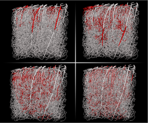
Figure 2. Flow rates and Péclet numbers within a mouse microvascular network, as computed in Cruz-Hernández et al. (Reference Cruz-Hernández, Bracko, Kersbergen, Muse, Haft-Javaherian, Berg, Park, Vinarcsik, Ivasyk and Kang2019). (a) Flow rates in a network that contains more than 15 000 vessels for a volume of approximately 1 cubic millimetre. It was obtained post mortem and imaged by two photon microscopy (Tsai et al. Reference Tsai, Kaufhold, Blinder, Friedman, Drew, Karten, Lyden and Kleinfeld2009; Blinder et al. Reference Blinder, Tsai, Kaufhold, Knutsen, Suhl and Kleinfeld2013). The topology is described by an adjacency matrix, storing the list of all edges (e.g.  $0$,
$0$,  $1$ and
  $2$) connected to a given vertex (e.g. B), as illustrated for a single bifurcation. (b) Distribution of the radial Péclet numbers,
  $\langle U\rangle R/D_{V}$, based on the blood flow distribution shown in (a) for a diffusion coefficient
  $D_{mol}=10^{-9}~\text{m}^{2}~\text{s}^{-1}$. Each dot represents a different vessel and the coloured surface shows the local density of points.
Developing such microvascular transport models is challenging. The main difficulty in doing so is to accurately capture the multiscale and multiphysics nature of the problem, which couples nonlinear effects in the rheology of blood (Pries et al. Reference Pries, Ley, Claassen and Gaehtgens1989; Pries & Secomb Reference Pries and Secomb2005), molecular transfers across complex biological tissues (Abbott et al. Reference Abbott, Patabendige, Dolman, Yusof and Begley2010; Kutuzov, Flyvbjerg & Lauritzen Reference Kutuzov, Flyvbjerg and Lauritzen2018) and effects linked to the geometry/topology of the vasculature (Lorthois & Cassot Reference Lorthois and Cassot2010). The most widespread approach to modelling such systems, is to consider each microvessel as a tube and the microvasculature as a network of connected tubes (illustrated in figure 2(a), see also Pries et al. (Reference Pries, Secomb, Gaehtgens and Gross1990), Goldman & Popel (Reference Goldman and Popel1999), Secomb et al. (Reference Secomb, Hsu, Park and Dewhirst2004), Fang et al. (Reference Fang, Sakadžić, Ruvinskaya, Devor, Dale and Boas2008), Obrist et al. (Reference Obrist, Weber, Buck and Jenny2010), Linninger et al. (Reference Linninger, Gould, Marinnan, Hsu, Chojecki and Alaraj2013), Kojic et al. (Reference Kojic, Milosevic, Simic, Koay, Fleming, Nizzero, Kojic, Ziemys and Ferrari2017), Peyrounette et al. (Reference Peyrounette, Davit, Quintard and Lorthois2018), and Sweeney, Walker-Samuel & Shipley (Reference Sweeney, Walker-Samuel and Shipley2018)). The advantage of this representation is that it simplifies the treatment of each vessel, making it possible to model large volumes and to capture the global topology of the network. The disadvantage, however, is that its accuracy heavily relies on the quality of the models used to represent each individual tube and the couplings between tubes. This framework is well established for blood flow (Pries et al. Reference Pries, Secomb, Gaehtgens and Gross1990; Lorthois, Cassot & Lauwers Reference Lorthois, Cassot and Lauwers2011; Fry et al. Reference Fry, Lee, Smith and Secomb2012) and accurately describes both in vivo and in vitro data (Pries & Secomb Reference Pries and Secomb2005; Cruz-Hernández et al. Reference Cruz-Hernández, Bracko, Kersbergen, Muse, Haft-Javaherian, Berg, Park, Vinarcsik, Ivasyk and Kang2019). However, we shall see that the same is not true of models of molecular transport (Goldman & Popel Reference Goldman and Popel1999; Secomb et al. Reference Secomb, Hsu, Park and Dewhirst2004; Fang et al. Reference Fang, Sakadžić, Ruvinskaya, Devor, Dale and Boas2008; Linninger et al. Reference Linninger, Gould, Marinnan, Hsu, Chojecki and Alaraj2013; Kojic et al. Reference Kojic, Milosevic, Simic, Koay, Fleming, Nizzero, Kojic, Ziemys and Ferrari2017; Sweeney et al. Reference Sweeney, Walker-Samuel and Shipley2018), which need to be improved. Most of them indeed rely on the well-mixed hypothesis and assume that radial gradients inside the blood vessels are negligible. The validity of this hypothesis requires detailed examination.
To illustrate this, let us first consider effective models of scalar transport in tubes, i.e. a larger class of problems that is central to many applications involving heat transfer, such as heat pipes in heat exchangers (Faghri Reference Faghri1995; Reay, Kew & McGlen Reference Reay, Kew and McGlen2014) or solute transport, such as microchannels in labs-on-chip (Bello, Rezzonico & Righetti Reference Bello, Rezzonico and Righetti1994; Weigl & Yager Reference Weigl and Yager1999; Beard Reference Beard2001). Since the influential works of Taylor (Reference Taylor1953) and Aris (Reference Aris1956), who focused on Poiseuille flow in impermeable straight cylinders, this problem has been extended to a large variety of configurations, including other velocity fields, e.g. Fan & Hwang (Reference Fan and Hwang1965) and Gentile, Ferrari & Decuzzi (Reference Gentile, Ferrari and Decuzzi2008), and more complex geometries, e.g. Brenner & Stewartson (Reference Brenner and Stewartson1980) and Koch & Brady (Reference Koch and Brady1985). Fundamental to scalar transport in a tube is the impact of radial gradients on the concentration field. These gradients, even if small in magnitude in the asymptotic regime, yield a huge increase in the longitudinal dispersion coefficient at sufficiently large Péclet numbers. For impermeable tubes, this is a consequence of the radial velocity gradient and the dispersion is often said to be shear induced or shear augmented. When the tube is permeable or semi-permeable, couplings between the scalar fields inside and outside the tube may yield additional gradients. In particular, sources or sinks in the domain surrounding the tube may generate strong radial concentration gradients within the tube. To study transport in the microcirculation, many authors (Reneau, Bruley & Knisely Reference Reneau, Bruley and Knisely1969; Levitt Reference Levitt1972; Bate, Rowlands & Sirs Reference Bate, Rowlands and Sirs1973; Lane & Sirs Reference Lane and Sirs1974; Hellums Reference Hellums1977; Tepper, Lee & Lightfoot Reference Tepper, Lee and Lightfoot1978; Lincoff, Borovetz & Inskeep Reference Lincoff, Borovetz and Inskeep1983; Baxter, Yuan & Jain Reference Baxter, Yuan and Jain1992; Fallon & Anuj Reference Fallon and Anuj2005; Grinberg et al. Reference Grinberg, Novozhilov, Grinberg, Friedman and Swartz2005; Secomb Reference Secomb2015) have considered a model axisymmetric system, called the Krogh cylinder, consisting of a single straight capillary surrounded by an annulus of tissue (Krogh Reference Krogh1919). For this model system, results in Levitt (Reference Levitt1972) and Lincoff et al. (Reference Lincoff, Borovetz and Inskeep1983) suggest that Péclet numbers are small in the capillary bed and therefore that dispersive effects are negligible. However, the Krogh cylinder overly simplifies the geometry of the microvasculature so that extrapolation to realistic cases is difficult. For instance, cumulative effects may occur within networks, where dispersion and intravascular gradients might become important only for a large system. Further, since the Péclet number scales with both the characteristic length of the problem and the average velocity within each vessel, dispersive effects may become important in arterioles and venules (Lincoff et al. Reference Lincoff, Borovetz and Inskeep1983) that are larger in diameter and where blood flows faster.
We argue that recent developments in microscopy techniques are a key element in assessing the validity of the well-mixed hypothesis. For example, in vivo data in Sakadžić et al. (Reference Sakadžić, Mandeville, Gagnon, Musacchia, Yaseen, Yucel, Lefebvre, Lesage and Dale2014) show radial gradients of oxygen within arterioles, therefore experimentally demonstrating that the well-mixed hypothesis is not always valid. Other experiments also allow us to re-evaluate the importance of dispersive effects. Multiphoton microscopy (Denk, Strickler & Webb Reference Denk, Strickler and Webb1990; Shih et al. Reference Shih, Driscoll, Drew, Nishimura, Schaffer and Kleinfeld2012), for example, can be used to determine the velocity within the brains of living rodents (Santisakultarm et al. Reference Santisakultarm, Cornelius, Nishimura, Schafer, Silver, Doerschuk, Olbricht and Schaffer2012; Taylor et al. Reference Taylor, Hui, Watson, Nie, Deardorff, Jensen, Helpern and Shih2016) and infer the distribution of Péclet numbers in microvascular networks. Another approach consists in combining large post mortem anatomical network geometries (Tsai et al. Reference Tsai, Kaufhold, Blinder, Friedman, Drew, Karten, Lyden and Kleinfeld2009) with simulations of blood flow (Schmid et al. Reference Schmid, Tsai, Kleinfeld, Jenny and Weber2017; Cruz-Hernández et al. Reference Cruz-Hernández, Bracko, Kersbergen, Muse, Haft-Javaherian, Berg, Park, Vinarcsik, Ivasyk and Kang2019) to calculate the velocity field throughout the network. Figure 2(b) shows the corresponding distribution of Péclet numbers for a molecule with high diffusivity ( $10^{-9}~\text{m}^{2}~\text{s}^{-1}$), which provides a lower bound for the Péclet numbers. It shows that most Péclet numbers are above 1 and suggests that, contrary to estimations made in Levitt (Reference Levitt1972) and Lincoff et al. (Reference Lincoff, Borovetz and Inskeep1983), Taylor’s dispersion may be important in a significant proportion of the smallest capillaries.
In this work, we use a theoretical approach to ask whether the well-mixed hypothesis is adapted to describing molecular transport in the brain microcirculation. Our goal is to understand how radial concentration gradients affect intravascular transport, mass fluxes throughout the blood–brain barrier and molecular uptake within the tissue. Our strategy is to focus on situations of weak couplings between the vessels and tissue, so that the vascular network can be treated independently from the tissue (§ 2). We first use multiscale asymptotics to identify such situations. Then, we derive a generic form of the transport model for cross-section-averaged concentrations in tubes (§ 3.1) and networks (§ 3.2). We finally study the impact of dimensionless parameters and velocity profile on effective coefficients (§ 4.1) and compare our model with the well-mixed hypothesis at vessel (§ 4.2) and network scale (§ 4.3).
2 Problem set-up
Here, we set up the modelling bases of the problem of solute transport. Our goal is to derive a network model for complex microvascular architectures. To this end, we first consider the case of a rigid, straight, long and narrow cylinder embedded in an infinite domain of tissue, as illustrated in figure 3. The solute can be metabolized within the tissue but behaves as a passive tracer in vessels, e.g. a nutrient. Following Pries et al. (Reference Pries, Secomb, Gaehtgens and Gross1990) and Secomb (Reference Secomb2017), the blood is considered as a continuous fluid. The vessel walls are supposed to act as a membrane, semi-permeable to solute and impermeable to fluid (Lorthois et al. Reference Lorthois, Duru, Billanou, Quintard and Celsis2014a; Kutuzov et al. Reference Kutuzov, Flyvbjerg and Lauritzen2018). We also assume that the tissue surrounding the vessel is a continuous medium with uniform properties (Levitt Reference Levitt1972; Lincoff et al. Reference Lincoff, Borovetz and Inskeep1983; Hellums et al. Reference Hellums, Nair, Huang and Ohshima1995; Goldman & Popel Reference Goldman and Popel1999; Secomb et al. Reference Secomb, Hsu, Park and Dewhirst2004; Fallon & Anuj Reference Fallon and Anuj2005; Fang et al. Reference Fang, Sakadžić, Ruvinskaya, Devor, Dale and Boas2008; Linninger et al. Reference Linninger, Gould, Marinnan, Hsu, Chojecki and Alaraj2013; Kojic et al. Reference Kojic, Milosevic, Simic, Koay, Fleming, Nizzero, Kojic, Ziemys and Ferrari2017; Sweeney et al. Reference Sweeney, Walker-Samuel and Shipley2018) where transport is mainly diffusive (Nicholson Reference Nicholson2001; Holter et al. Reference Holter, Kehlet, Devor, Sejnowski, Dale, Omholt, Ottersen, Nagelhus, Mardal and Pettersen2017; Kutuzov et al. Reference Kutuzov, Flyvbjerg and Lauritzen2018). Since the aspect ratio (radius over length) of the vessel is small, the flow is treated as invariant along the vessel length and the velocity profile is independent of the axial position along the vessel. Using these hypotheses, we first write the mass balance equations within the vessel and tissue (§§ 2.1 and 2.2). Then we use multiscale asymptotics to describe the different transport regimes and identify situations of weak coupling where the vessel can be treated separately from the tissue (§ 2.3).

Figure 3. Schematic of solute transport within a single capillary. Here  $C_{V}$ is the local concentration of solute within the vessel and
  $C_{T}$ the local concentration within the tissue.
  $U(r)$ represents the velocity profile;
  $D_{V}$ the diffusion coefficient of the solute within the vessel;
  $K_{m}$ is the membrane permeability;
  $D_{T}$ denotes the diffusion coefficient within the tissue; and
  $M(C_{T})$ the consumption rate of solute within the tissue.
2.1 Microscopic transport equations and boundary conditions
In order to derive the three-dimensional (3-D) local transport equations for the concentration within both vessels and tissue, we consider a binary solvent/solute mixture in each domain. The diffusion flux in vessels and tissue is determined using Fick’s first law. With these assumptions, the mass balance equation for solute within vessels can be written as
 $$\begin{eqnarray}\unicode[STIX]{x2202}_{t}(\unicode[STIX]{x1D70C}_{V}Y_{V})=\unicode[STIX]{x1D735}\boldsymbol{\cdot }(-\unicode[STIX]{x1D70C}_{V}\boldsymbol{U}Y_{V}+\unicode[STIX]{x1D70C}_{V}D_{V}\unicode[STIX]{x1D735}Y_{V}),\end{eqnarray}$$
 where  $\unicode[STIX]{x1D70C}_{V}$ is the local mass density in the vessel
  $(\text{kg}~\text{m}^{-3})$,
  $Y_{V}$ the local solute mass fraction,
  $\boldsymbol{U}$ the local velocity
  $(\text{m}~\text{s}^{-1})$ and
  $D_{V}$ the molecular diffusion coefficient
  $(\text{m}^{2}~\text{s}^{-1})$ of the solute in vessels.
Transport in the tissue is mainly diffusive so that we have
 $$\begin{eqnarray}\unicode[STIX]{x2202}_{t}(\unicode[STIX]{x1D70C}_{T}Y_{T})=\unicode[STIX]{x1D735}\boldsymbol{\cdot }(\unicode[STIX]{x1D70C}_{T}D_{T}\unicode[STIX]{x1D735}Y_{T})-M,\end{eqnarray}$$
 where  $\unicode[STIX]{x1D70C}_{T}$ is the local density of the tissue
  $(\text{kg}~\text{m}^{-3})$,
  $Y_{T}$ the local solute mass fraction,
  $D_{T}$ is the molecular diffusion coefficient
  $(\text{m}^{2}~\text{s}^{-1})$ of the solute within the tissue and
  $M$ the local metabolic reaction rate
  $(\text{kg}~\text{m}^{-3}~\text{s}^{-1})$. Here,
  $D_{V}\neq D_{T}$ and both are assumed to be uniform and constant. We consider that the solute is dilute and does not modify the densities. We can therefore write
 $$\begin{eqnarray}\displaystyle & \displaystyle C_{V}=\unicode[STIX]{x1D70C}_{V}Y_{V}, & \displaystyle\end{eqnarray}$$
 $$\begin{eqnarray}\displaystyle & \displaystyle C_{T}=\unicode[STIX]{x1D70C}_{T}Y_{T}, & \displaystyle\end{eqnarray}$$
 where  $\unicode[STIX]{x1D70C}_{V}$ and
  $\unicode[STIX]{x1D70C}_{T}$ are uniform and constant and
  $C_{V}$ and
  $C_{T}$ are the local mass concentration
  $(\text{kg}~\text{m}^{-3})$. Hence, equations (2.1) and (2.2) now yield
 $$\begin{eqnarray}\displaystyle & \displaystyle \unicode[STIX]{x2202}_{t}C_{V}=\unicode[STIX]{x1D735}\boldsymbol{\cdot }(-\boldsymbol{U}C_{V}+D_{V}\unicode[STIX]{x1D735}C_{V}), & \displaystyle\end{eqnarray}$$
 $$\begin{eqnarray}\displaystyle & \displaystyle \unicode[STIX]{x2202}_{t}C_{T}=\unicode[STIX]{x1D735}\boldsymbol{\cdot }(D_{T}\unicode[STIX]{x1D735}C_{T})-M, & \displaystyle\end{eqnarray}$$
which are the local transport equation for the concentration of solute within the vessels and tissue.
The metabolic reaction rate  $M$ is modelled using a Michaelis–Menten kinetics, which is standard for oxygen (Secomb et al. Reference Secomb, Hsu, Park and Dewhirst2004) or glucose (Atkins & De Paula Reference Atkins and De Paula2011). Consequently, equation (2.6) becomes
 $$\begin{eqnarray}\unicode[STIX]{x2202}_{t}C_{T}=\unicode[STIX]{x1D735}\boldsymbol{\cdot }(D_{T}\unicode[STIX]{x1D735}C_{T})-M_{T}\frac{C_{T}}{C_{0}+C_{T}},\end{eqnarray}$$
 where  $M_{T}$ is the maximal metabolic rate
  $(\text{kg}~\text{m}^{-3}~\text{s}^{-1})$ and
  $C_{0}$ the concentration
  $(\text{kg}~\text{m}^{-3})$ at which the metabolic reaction term equals half its maximal value.
Finally, the vessels and tissue are coupled together through the blood–brain barrier. We treat this barrier as a geometric manifold (infinitely thin layer) with transmission boundary conditions connecting the two domains. Assuming that there is no sorption of solute molecule onto the barrier, mass conservation reads
 $$\begin{eqnarray}-\boldsymbol{n}\boldsymbol{\cdot }(D_{V}\unicode[STIX]{x1D735}C_{V})=-\boldsymbol{n}\boldsymbol{\cdot }(D_{T}\unicode[STIX]{x1D735}C_{T}),\end{eqnarray}$$
 where  $\boldsymbol{n}$ is the unit normal vector pointing outward from the vessel. To represent the selective action of the blood–brain barrier, we use a membrane condition in the form
 $$\begin{eqnarray}-\boldsymbol{n}\boldsymbol{\cdot }(D_{V}\unicode[STIX]{x1D735}C_{V})=K_{m}(C_{V}-\unicode[STIX]{x1D706}C_{T}),\end{eqnarray}$$
 with  $K_{m}$ the membrane permeability
  $(\text{m}~\text{s}^{-1})$. Here,
  $K_{m}$ is primarily introduced as a parameter allowing us to model the ability of a given molecule to pass the barrier. The limit
  $K_{m}\rightarrow 0$ corresponds to a molecule that cannot pass the barrier, resulting in a homogeneous Neumann boundary condition. On the other hand,
  $K_{m}\rightarrow \infty$ leads to
  $C_{V}=\unicode[STIX]{x1D706}C_{T}$, which corresponds to thermodynamic equilibrium and may be obtained through equality of chemical potentials with
  $\unicode[STIX]{x1D706}$ the partition coefficient (Atkins & De Paula Reference Atkins and De Paula2011). This boundary condition, which is analogous to the thermal resistance in heat transfer, is widely used in microcirculation (Lincoff et al. Reference Lincoff, Borovetz and Inskeep1983; Fang et al. Reference Fang, Sakadžić, Ruvinskaya, Devor, Dale and Boas2008; Vikhansky & Wang Reference Vikhansky and Wang2011; Sweeney et al. Reference Sweeney, Walker-Samuel and Shipley2018) and captures the selectivity of blood/tissue exchanges through the blood–brain barrier.
2.2 Non-dimensionalization of transport equations
The local transport problem, equations (2.5) and (2.7)–(2.9), is non-dimensionalized using the characteristic vessel length,  $L$, and the associated diffusive time scale,
  $L^{2}/D_{V}$. The concentration field is non-dimensionalized using
  $C_{inlet}$ in the vessel and
  $C_{0}$ in the tissue. Here,
  $C_{inlet}$ corresponds to the concentration at the vessel inlet and
  $C_{0}$ to the concentration at which the metabolic reaction term equals half its maximal value. The dimensionless initial-boundary value problem now reads
 $$\begin{eqnarray}\displaystyle & \displaystyle \unicode[STIX]{x2202}_{t}C_{V}=-Pe\unicode[STIX]{x1D735}\boldsymbol{\cdot }(\boldsymbol{U}^{\ast }C_{V})+\unicode[STIX]{x1D6FB}^{2}C_{V}, & \displaystyle\end{eqnarray}$$
 $$\begin{eqnarray}\displaystyle & \displaystyle \unicode[STIX]{x2202}_{t}C_{T}=\unicode[STIX]{x1D702}\unicode[STIX]{x1D6FB}^{2}C_{T}-\unicode[STIX]{x1D702}Da_{T}\frac{C_{T}}{1+C_{T}}, & \displaystyle\end{eqnarray}$$
 $$\begin{eqnarray}\displaystyle & \displaystyle -\boldsymbol{n}\boldsymbol{\cdot }\unicode[STIX]{x1D735}C_{V}=-\boldsymbol{n}\boldsymbol{\cdot }(\unicode[STIX]{x1D702}\unicode[STIX]{x1D6FE}\unicode[STIX]{x1D735}C_{T}), & \displaystyle\end{eqnarray}$$
 $$\begin{eqnarray}\displaystyle & \displaystyle -\boldsymbol{n}\boldsymbol{\cdot }\unicode[STIX]{x1D735}C_{V}=Da_{m}(C_{V}-\unicode[STIX]{x1D706}\unicode[STIX]{x1D6FE}C_{T}), & \displaystyle\end{eqnarray}$$
 where  $Pe=\langle U\rangle L/D_{V}$ is the longitudinal Péclet number based on the cross-section-averaged velocity
  $\langle U\rangle =(1/\unicode[STIX]{x03C0}R^{2})\iint \boldsymbol{U}\boldsymbol{\cdot }\boldsymbol{n}\,\text{d}S$ and
  $\boldsymbol{U}^{\ast }=\boldsymbol{U}/\langle U\rangle$ is the normalized velocity;
  $Da_{T}=M_{T}L^{2}/C_{0}D_{T}$ is the longitudinal Damköhler number within the tissue;
  $\unicode[STIX]{x1D702}=D_{T}/D_{V}$ is the diffusivity ratio;
  $Da_{m}=K_{m}L/D_{V}$ is the longitudinal membrane Damköhler number; and
  $\unicode[STIX]{x1D6FE}=C_{0}/C_{inlet}$ is the ratio of reference concentrations. The corresponding radial Péclet and Damköhler numbers, based on the cylinder radius instead of its length, are
 $$\begin{eqnarray}Pe_{radial}=\unicode[STIX]{x1D716}Pe,\quad Da_{T,radial}=\unicode[STIX]{x1D716}^{2}Da_{T},\quad Da_{m,radial}=\unicode[STIX]{x1D716}Da_{m},\end{eqnarray}$$
where
 $$\begin{eqnarray}\unicode[STIX]{x1D716}=\frac{R}{L}\end{eqnarray}$$
is the aspect ratio of the tube.
2.3 Asymptotic transport regimes
Due to the strong couplings between the vessel and tissue, it is not possible to derive a general 1-D effective transport equation for the cross-section-averaged concentration inside the vessel by simply averaging equation (2.10). As mentioned in the Introduction, one way to obtain such an effective model is to consider a subset of possible geometries, e.g. the Krogh cylinder. The main drawback of this approach is that it makes generalization to realistic microvascular architectures difficult. Another alternative is to identify regimes where couplings between the vessel and the tissue are relatively weak, so that the transport within each vessel can be treated as independent of the transport within the tissue. To this end, we use multiscale asymptotics (Bensoussan, Lions & Papanicolaou Reference Bensoussan, Lions and Papanicolaou1978; Davit et al. Reference Davit, Bell, Byrne, Chapman, Kimpton, Lang, Leonard, Oliver, Pearson and Shipley2013) to identify the specific scalings of the control parameters, expressed as powers of  $\unicode[STIX]{x1D716}$ (e.g.
  $Pe=O(\unicode[STIX]{x1D716}^{i})$), that yield weak couplings. In the following, we will further assume that, for small molecules like water, oxygen or nutrients,
  $\unicode[STIX]{x1D706}=O(1)$ and
  $\unicode[STIX]{x1D702}=O(1)$. In addition, we suppose that the characteristic concentration in the tissue is small compared to the characteristic concentration inside the vessel, so that
  $\unicode[STIX]{x1D6FE}=O(\unicode[STIX]{x1D716})$, as it is the case for oxygen (Sweeney et al. Reference Sweeney, Walker-Samuel and Shipley2018). Doing so reduces the set of dimensionless numbers, for a given geometry, to
  $Pe$,
$Pe$,  $Da_{T}$ and
  $Da_{m}$.
For the cylindrical geometry at hand (figure 3), the spatial differential operators have the following expressions:
 $$\begin{eqnarray}\displaystyle & \displaystyle \unicode[STIX]{x1D735}\bullet =\boldsymbol{e}_{\boldsymbol{r}}\unicode[STIX]{x2202}_{r}\bullet +\boldsymbol{e}_{\boldsymbol{z}}\unicode[STIX]{x2202}_{z}\bullet , & \displaystyle\end{eqnarray}$$
 $$\begin{eqnarray}\displaystyle & \displaystyle \unicode[STIX]{x1D6FB}^{2}\bullet =\frac{1}{r}\unicode[STIX]{x2202}_{r}(r\unicode[STIX]{x2202}_{r}\bullet )+\unicode[STIX]{x2202}_{z}^{2}\bullet , & \displaystyle\end{eqnarray}$$
 with  $\boldsymbol{e}_{\boldsymbol{r}}$ and
  $\boldsymbol{e}_{\boldsymbol{z}}$ the unit vectors associated with the transverse and longitudinal directions. In such a configuration, there are primarily two scales of variations for the differential operators, the longitudinal scale
  $z$ and the transverse scale
  $r$. In order to highlight those scales in (2.16) and (2.17), we rescale the radial coordinate and introduce the following change of variable:
 $$\begin{eqnarray}\unicode[STIX]{x1D716}\unicode[STIX]{x1D70C}=r.\end{eqnarray}$$
Equations (2.16) and (2.17) then become
 $$\begin{eqnarray}\displaystyle & \displaystyle \unicode[STIX]{x1D735}\bullet =\unicode[STIX]{x1D716}^{-1}\boldsymbol{e}_{\boldsymbol{r}}\unicode[STIX]{x2202}_{\unicode[STIX]{x1D70C}}\bullet +\boldsymbol{e}_{\boldsymbol{z}}\unicode[STIX]{x2202}_{z}\bullet , & \displaystyle\end{eqnarray}$$
 $$\begin{eqnarray}\displaystyle & \displaystyle \unicode[STIX]{x1D6FB}^{2}\bullet =\unicode[STIX]{x1D716}^{-2}\frac{1}{\unicode[STIX]{x1D70C}}\unicode[STIX]{x2202}_{\unicode[STIX]{x1D70C}}(\unicode[STIX]{x1D70C}\unicode[STIX]{x2202}_{\unicode[STIX]{x1D70C}}\bullet )+\unicode[STIX]{x2202}_{z}^{2}\bullet . & \displaystyle\end{eqnarray}$$
For the rest of this section, we therefore define the following notations:
 $$\begin{eqnarray}\unicode[STIX]{x1D735}\bullet =\unicode[STIX]{x1D735}_{z}\bullet +\unicode[STIX]{x1D716}^{-1}\unicode[STIX]{x1D735}_{\unicode[STIX]{x1D70C}}\bullet\end{eqnarray}$$
and
 $$\begin{eqnarray}\unicode[STIX]{x1D6FB}^{2}\bullet =\unicode[STIX]{x1D6FB}_{z}^{2}\bullet +\unicode[STIX]{x1D716}^{-2}\unicode[STIX]{x1D6FB}_{\unicode[STIX]{x1D70C}}^{2}\bullet .\end{eqnarray}$$
 The main idea is then to separate the length scales of variation of the concentration fields in both vessel and tissue into different components and search for solutions in the form of series of powers of  $\unicode[STIX]{x1D716}$
 $$\begin{eqnarray}C_{X}=\mathop{\sum }_{i}\unicode[STIX]{x1D716}^{i}C_{X,i}(r,z,t)\quad X=V,T.\end{eqnarray}$$
Injecting the above derivative expressions and the series form of the solution into the transport equations within vessel and tissues ((2.10) and (2.13)) yields
 $$\begin{eqnarray}\displaystyle & & \displaystyle \mathop{\sum }_{i}\unicode[STIX]{x1D716}^{i}\unicode[STIX]{x2202}_{t}C_{V,i}\nonumber\\ \displaystyle & & \displaystyle \quad =\mathop{\sum }_{i}\unicode[STIX]{x1D716}^{i}(-Pe(\unicode[STIX]{x1D735}_{z}\boldsymbol{\cdot }(\boldsymbol{U}^{\ast }C_{V,i})+\unicode[STIX]{x1D716}^{-1}\unicode[STIX]{x1D735}_{\unicode[STIX]{x1D70C}}\boldsymbol{\cdot }(\boldsymbol{U}^{\ast }C_{V,i}))+\unicode[STIX]{x1D6FB}_{z}^{2}C_{V,i}+\unicode[STIX]{x1D716}^{-2}\unicode[STIX]{x1D6FB}_{\unicode[STIX]{x1D70C}}^{2}C_{V,i}),\qquad\end{eqnarray}$$
 $$\begin{eqnarray}\mathop{\sum }_{i}\unicode[STIX]{x1D716}^{i}\unicode[STIX]{x2202}_{t}C_{T,i}=\mathop{\sum }_{i}\unicode[STIX]{x1D716}^{i}\left(\unicode[STIX]{x1D702}\unicode[STIX]{x1D6FB}_{z}^{2}C_{T,i}+\unicode[STIX]{x1D716}^{-2}\unicode[STIX]{x1D702}\unicode[STIX]{x1D6FB}_{\unicode[STIX]{x1D70C}}^{2}C_{T,i}-\unicode[STIX]{x1D702}Da_{T}\frac{C_{T,i}}{\displaystyle 1+\mathop{\sum }_{k}\unicode[STIX]{x1D716}^{k}C_{T,k}}\right).\end{eqnarray}$$
Doing the same for the boundary conditions at the vessel wall leads to
 $$\begin{eqnarray}\displaystyle & \displaystyle -\mathop{\sum }_{i}\unicode[STIX]{x1D716}^{i}\boldsymbol{n}\boldsymbol{\cdot }(\unicode[STIX]{x1D735}_{z}C_{V,i}+\unicode[STIX]{x1D716}^{-1}\unicode[STIX]{x1D735}_{\unicode[STIX]{x1D70C}}C_{V,i})=-\mathop{\sum }_{i}\unicode[STIX]{x1D716}^{i}\boldsymbol{n}\boldsymbol{\cdot }\unicode[STIX]{x1D702}\unicode[STIX]{x1D6FE}(\unicode[STIX]{x1D735}_{z}C_{T,i}+\unicode[STIX]{x1D716}^{-1}\unicode[STIX]{x1D735}_{\unicode[STIX]{x1D70C}}C_{T,i}), & \displaystyle\end{eqnarray}$$
 $$\begin{eqnarray}\displaystyle & \displaystyle -\mathop{\sum }_{i}\unicode[STIX]{x1D716}^{i}\boldsymbol{n}\boldsymbol{\cdot }(\unicode[STIX]{x1D735}_{z}C_{V,i}+\unicode[STIX]{x1D716}^{-1}\unicode[STIX]{x1D735}_{\unicode[STIX]{x1D70C}}C_{V,i})=\mathop{\sum }_{i}\unicode[STIX]{x1D716}^{i}(Da_{m}(C_{V,i}-\unicode[STIX]{x1D706}\unicode[STIX]{x1D6FE}C_{T,i})). & \displaystyle\end{eqnarray}$$
 In (2.24), we have  $\unicode[STIX]{x1D716}^{-1}\unicode[STIX]{x1D735}_{\unicode[STIX]{x1D70C}}\boldsymbol{\cdot }(\boldsymbol{U}^{\ast }C_{V,i})=0$ since there is only axial convection. Similarly, in (2.26) and (2.27) the terms
  $\boldsymbol{n}\boldsymbol{\cdot }\unicode[STIX]{x1D735}_{z}C_{V,i}$ and
  $\boldsymbol{n}\boldsymbol{\cdot }\unicode[STIX]{x1D735}_{z}C_{T,i}$ vanish as
  $\boldsymbol{n}$ (here
  $\boldsymbol{e}_{\boldsymbol{r}}$) is orthogonal to
  $\unicode[STIX]{x1D735}_{z}\bullet$ (here
  $\boldsymbol{e}_{\boldsymbol{z}}\unicode[STIX]{x2202}_{z}\bullet$).
For each set of scalings of the dimensionless parameters ( $Pe$,
$Pe$,  $Da_{T}$,
  $Da_{m}$), we obtain a nested sequence of subproblems corresponding to the different powers of
  $\unicode[STIX]{x1D716}$, which allows us to identify the leading-order concentration fields (
 $C_{V,0}$,
  $C_{V,1}$,
  $C_{T,0}$,
  $C_{T,1}$). Effective transport equations for the cross-section-averaged concentration are then obtained by averaging the resulting equations in space via the following operator:
 $$\begin{eqnarray}\langle \bullet \rangle =\frac{1}{\unicode[STIX]{x03C0}\unicode[STIX]{x1D716}^{2}}\iint \bullet r\,\text{d}r\,\text{d}\unicode[STIX]{x1D703}=\frac{1}{\unicode[STIX]{x03C0}}\iint \bullet \unicode[STIX]{x1D70C}\,\text{d}\unicode[STIX]{x1D70C}\,\text{d}\unicode[STIX]{x1D703}\end{eqnarray}$$
so that in general
 $$\begin{eqnarray}\langle C_{V}\rangle =\mathop{\sum }_{i}\unicode[STIX]{x1D716}^{i}\langle C_{V,i}\rangle .\end{eqnarray}$$
 For concision, this cross-section-averaged concentration  $\langle C_{V}\rangle$ is simply referred to as the average concentration in the rest of this paper. Inspired by the work of Mei (Reference Mei1992), Auriault & Adler (Reference Auriault and Adler1995) and Allaire et al. (Reference Allaire, Brizzi, Mikelić and Piatnitski2010), we illustrate how this approach can be used to obtain the well-known regime of Taylor’s dispersion. We show that, in this case, the boundary conditions ((2.12) and (2.13)) degenerate into Neuman boundary conditions, consistent with the impermeable walls of Taylor’s case (§ 2.3.1). Then, we go on to generalize this study to a large range of parameter scalings and to identify the regimes in phase space that correspond to weak vessel–tissue couplings (§ 2.3.2). For all these scalings, we further show that the membrane boundary condition (2.13) degenerates into a Robin-type boundary condition at the vessel walls.
2.3.1 Recovering Taylor’s dispersion
Taylor’s dispersion is obtained when molecules primarily remain inside the vessels and the Péclet number is large enough. The corresponding set of scalings reads
 $$\begin{eqnarray}Pe=O(\unicode[STIX]{x1D716}^{-1}),\quad Da_{m}=O(\unicode[STIX]{x1D716}^{2}),\quad Da_{T}=O(\unicode[STIX]{x1D716}^{-3}).\end{eqnarray}$$
Because the Péclet number is large, it is necessary to decompose the time derivative within the vessel using two time scales to capture both the contributions of longitudinal convection and longitudinal diffusion to the effective transport. This reads
 $$\begin{eqnarray}\unicode[STIX]{x2202}_{t}\bullet =\unicode[STIX]{x2202}_{t^{\ast }}\bullet +Pe\unicode[STIX]{x2202}_{\unicode[STIX]{x1D70F}}\bullet ,\end{eqnarray}$$
 where  $t^{\ast }$ corresponds to the time variation of longitudinal diffusion and
  $\unicode[STIX]{x1D70F}$ corresponds to the time variation of longitudinal convection.
In addition,  $Da_{T}=O(\unicode[STIX]{x1D716}^{-3})$ implies that the tissue Damköhler is very large. In such a regime, we expect the concentration in the tissue to be small so that the reaction rate can be approximated by a first-order kinetics. Note that taking into account the nonlinearity in the reaction rate does not change the results and only leads to tedious additional calculations that are not necessary for understanding the procedure. For this set of parameters, in the limit
  $\unicode[STIX]{x1D716}\rightarrow 0$, equations (2.24) and (2.25) lead to
 $$\begin{eqnarray}\displaystyle & \displaystyle C_{T,0}=0\quad O(\unicode[STIX]{x1D716}^{-3}), & \displaystyle\end{eqnarray}$$
 $$\begin{eqnarray}\displaystyle & \displaystyle \left.\begin{array}{@{}c@{}}\unicode[STIX]{x1D6FB}_{\unicode[STIX]{x1D70C}}^{2}C_{V,0}=0\\ \unicode[STIX]{x1D702}\unicode[STIX]{x1D6FB}_{\unicode[STIX]{x1D70C}}^{2}C_{T,0}-\unicode[STIX]{x1D702}(\unicode[STIX]{x1D716}^{3}Da_{T})C_{T,1}=0\end{array}\right\}\quad O(\unicode[STIX]{x1D716}^{-2}), & \displaystyle\end{eqnarray}$$
 $$\begin{eqnarray}\displaystyle & \displaystyle \left.\begin{array}{@{}c@{}}(\unicode[STIX]{x1D716}Pe)\unicode[STIX]{x2202}_{\unicode[STIX]{x1D70F}}C_{V,0}=-(\unicode[STIX]{x1D716}Pe)\unicode[STIX]{x1D735}_{z}\boldsymbol{\cdot }(\boldsymbol{U}^{\ast }C_{V,0})+\unicode[STIX]{x1D6FB}_{\unicode[STIX]{x1D70C}}^{2}C_{V,1}\\ \unicode[STIX]{x1D702}\unicode[STIX]{x1D6FB}_{\unicode[STIX]{x1D70C}}^{2}C_{T,1}-\unicode[STIX]{x1D702}(\unicode[STIX]{x1D716}^{3}Da_{T})C_{T,2}=0\end{array}\right\}\quad O(\unicode[STIX]{x1D716}^{-1}), & \displaystyle\end{eqnarray}$$
 $$\begin{eqnarray}\displaystyle & \displaystyle \left.\begin{array}{@{}c@{}}\unicode[STIX]{x2202}_{t^{\ast }}C_{V,0}+(\unicode[STIX]{x1D716}Pe)\unicode[STIX]{x2202}_{\unicode[STIX]{x1D70F}}C_{V,1}=-(\unicode[STIX]{x1D716}Pe)\unicode[STIX]{x1D735}_{z}\boldsymbol{\cdot }(\boldsymbol{U}^{\ast }C_{V,1})+\unicode[STIX]{x1D6FB}_{z}^{2}C_{V,0}+\unicode[STIX]{x1D6FB}_{\unicode[STIX]{x1D70C}}^{2}C_{V,2}\\ \unicode[STIX]{x2202}_{t}C_{T,0}=\unicode[STIX]{x1D702}\unicode[STIX]{x1D6FB}_{z}^{2}C_{T,0}+\unicode[STIX]{x1D702}\unicode[STIX]{x1D6FB}_{\unicode[STIX]{x1D70C}}^{2}C_{T,2}-\unicode[STIX]{x1D702}(\unicode[STIX]{x1D716}^{3}Da_{T})C_{T,3}\end{array}\right\}O(1). & \displaystyle\end{eqnarray}$$
Equation (2.26) becomes
 $$\begin{eqnarray}\displaystyle & \displaystyle -\boldsymbol{n}\boldsymbol{\cdot }\unicode[STIX]{x1D735}_{\unicode[STIX]{x1D70C}}C_{V,0}=0, & \displaystyle\end{eqnarray}$$
 $$\begin{eqnarray}\displaystyle & \displaystyle -\boldsymbol{n}\boldsymbol{\cdot }\unicode[STIX]{x1D735}_{\unicode[STIX]{x1D70C}}C_{V,i}=-\unicode[STIX]{x1D702}(\unicode[STIX]{x1D716}^{-1}\unicode[STIX]{x1D6FE})\boldsymbol{n}\boldsymbol{\cdot }\unicode[STIX]{x1D735}_{\unicode[STIX]{x1D70C}}C_{T,i-1},\quad i>0, & \displaystyle\end{eqnarray}$$
and equation (2.27)
 $$\begin{eqnarray}\displaystyle & \displaystyle -\boldsymbol{n}\boldsymbol{\cdot }\unicode[STIX]{x1D735}_{\unicode[STIX]{x1D70C}}C_{V,i}=0,\quad i\leqslant 2, & \displaystyle\end{eqnarray}$$
 $$\begin{eqnarray}\displaystyle & \displaystyle -\boldsymbol{n}\boldsymbol{\cdot }\unicode[STIX]{x1D735}_{\unicode[STIX]{x1D70C}}C_{V,3}=(\unicode[STIX]{x1D716}^{-2}Da_{m})C_{V,0},\quad i=3. & \displaystyle\end{eqnarray}$$
 $$\begin{eqnarray}\displaystyle & \displaystyle -\boldsymbol{n}\boldsymbol{\cdot }\unicode[STIX]{x1D735}_{\unicode[STIX]{x1D70C}}C_{V,i}=(\unicode[STIX]{x1D716}^{-2}Da_{m})(C_{V,i-3}-\unicode[STIX]{x1D706}(\unicode[STIX]{x1D716}^{-1}\unicode[STIX]{x1D6FE})C_{T,i-4}),\quad i>3. & \displaystyle\end{eqnarray}$$
 By mathematical induction, we obtain that  $C_{T,i}=0\;\forall i\in \mathbb{N}$ inside the tissue, so that the problem is fully controlled by intravascular transport. Equation (2.38) further shows that, at leading order, there is no diffusive flux at the vessel/tissue interface so that the membrane boundary condition degenerates into a homogeneous Neumann condition. Therefore, the model is equivalent to an impermeable wall, which obviously removes all vessel/tissue couplings and corresponds to Taylor’s dispersion regime. The effective transport equation is obtained by averaging equation (2.35) using the operator defined in (2.28). This leads to
 $$\begin{eqnarray}\unicode[STIX]{x2202}_{t^{\ast }}\langle C_{V,0}\rangle +\unicode[STIX]{x1D716}Pe\unicode[STIX]{x2202}_{\unicode[STIX]{x1D70F}}\langle C_{V,1}\rangle =-\unicode[STIX]{x1D716}Pe\unicode[STIX]{x1D735}_{z}\boldsymbol{\cdot }\langle \boldsymbol{U}^{\ast }C_{V,1}\rangle +\unicode[STIX]{x1D6FB}_{z}^{2}\langle C_{V,0}\rangle +\langle \unicode[STIX]{x1D6FB}_{\unicode[STIX]{x1D70C}}^{2}C_{V,2}\rangle ,\end{eqnarray}$$
 which can be further simplified by noticing that  $\langle \unicode[STIX]{x1D6FB}_{\unicode[STIX]{x1D70C}}^{2}C_{V,2}\rangle =0$ using the divergence theorem and the boundary condition at the vessel wall (2.38). To obtain an expression for
  $\langle \boldsymbol{U}^{\ast }C_{V,1}\rangle$ in (2.41), we consider equation (2.33) and use the divergence theorem to obtain
  $C_{V,0}=C_{V,0}(z)$. Therefore, equation (2.34) can be written as
 $$\begin{eqnarray}(\unicode[STIX]{x1D716}Pe)\unicode[STIX]{x2202}_{\unicode[STIX]{x1D70F}}C_{V,0}=-(\unicode[STIX]{x1D716}Pe)\boldsymbol{U}^{\ast }(\unicode[STIX]{x1D70C})\boldsymbol{\cdot }\unicode[STIX]{x1D735}_{z}C_{V,0}+\unicode[STIX]{x1D6FB}_{\unicode[STIX]{x1D70C}}^{2}C_{V,1}.\end{eqnarray}$$
Averaging equation (2.34) leads to
 $$\begin{eqnarray}(\unicode[STIX]{x1D716}Pe)\unicode[STIX]{x2202}_{\unicode[STIX]{x1D70F}}\langle C_{V,0}\rangle =-(\unicode[STIX]{x1D716}Pe)\langle \boldsymbol{U}^{\ast }\rangle \boldsymbol{\cdot }\unicode[STIX]{x1D735}_{z}\langle C_{V,0}\rangle .\end{eqnarray}$$
 We have already shown that  $C_{V,0}=C_{V,0}(z)$, which implies that
  $\langle C_{V,0}\rangle =C_{V,0}$. Consequently, we can subtract (2.43) from (2.42) to obtain
 $$\begin{eqnarray}(\unicode[STIX]{x1D716}Pe)\tilde{\boldsymbol{U}}(\unicode[STIX]{x1D70C})\boldsymbol{\cdot }\unicode[STIX]{x1D735}_{z}C_{V,0}=\unicode[STIX]{x1D6FB}_{\unicode[STIX]{x1D70C}}^{2}C_{V,1},\end{eqnarray}$$
 where  $\tilde{\boldsymbol{U}}=\boldsymbol{U}^{\ast }-\langle \boldsymbol{U}^{\ast }\rangle$ is the local perturbation of the velocity field. We then have a solution in the form
 $$\begin{eqnarray}C_{V,1}=(\unicode[STIX]{x1D716}Pe)\boldsymbol{b}(\unicode[STIX]{x1D70C})\boldsymbol{\cdot }\unicode[STIX]{x1D735}_{z}C_{V,0},\end{eqnarray}$$
 where  $\boldsymbol{b}$ is the closure variable which solves
 $$\begin{eqnarray}\displaystyle & \displaystyle \tilde{\boldsymbol{U}}=\unicode[STIX]{x1D6FB}_{\unicode[STIX]{x1D70C}}^{2}\boldsymbol{b}, & \displaystyle\end{eqnarray}$$
 $$\begin{eqnarray}\displaystyle & \displaystyle \boldsymbol{n}\boldsymbol{\cdot }\unicode[STIX]{x1D735}_{\unicode[STIX]{x1D70C}}\boldsymbol{b}=\mathbf{0}, & \displaystyle\end{eqnarray}$$
with uniqueness obtained via the average constraint
 $$\begin{eqnarray}\langle \boldsymbol{b}\rangle =0.\end{eqnarray}$$
In this regime, the definition of the average concentration implies that
 $$\begin{eqnarray}\left.\begin{array}{@{}c@{}}\langle C_{V}\rangle =\langle C_{V,0}\rangle ,\\ \langle C_{V,1}\rangle =0,\end{array}\right\}\end{eqnarray}$$
so that injecting (2.45) into (2.41) leads to
 $$\begin{eqnarray}\unicode[STIX]{x2202}_{t^{\ast }}\langle C_{V}\rangle =(1-\unicode[STIX]{x1D716}^{2}Pe^{2}\langle \boldsymbol{U}^{\ast }\boldsymbol{\cdot }\boldsymbol{b}\rangle )\unicode[STIX]{x1D6FB}_{z}^{2}\langle C_{V}\rangle .\end{eqnarray}$$
 Now, substituting  $\unicode[STIX]{x2202}_{t^{\ast }}\langle C_{V}\rangle$ using (2.31) yields
 $$\begin{eqnarray}\unicode[STIX]{x2202}_{t}\langle C_{V}\rangle =Pe\unicode[STIX]{x2202}_{\unicode[STIX]{x1D70F}}\langle C_{V}\rangle +(1-\unicode[STIX]{x1D716}^{2}Pe^{2}\langle \boldsymbol{U}^{\ast }\boldsymbol{\cdot }\boldsymbol{b}\rangle )\unicode[STIX]{x1D6FB}_{z}^{2}\langle C_{V}\rangle .\end{eqnarray}$$
Finally, using (2.43) in the above expression leads to
 $$\begin{eqnarray}\unicode[STIX]{x2202}_{t}\langle C_{V}\rangle =-Pe\langle \boldsymbol{U}^{\ast }\rangle \boldsymbol{\cdot }\unicode[STIX]{x1D735}_{z}\langle C_{V}\rangle +(1-\unicode[STIX]{x1D716}^{2}Pe^{2}\langle \boldsymbol{U}^{\ast }\boldsymbol{\cdot }\boldsymbol{b}\rangle )\unicode[STIX]{x1D6FB}_{z}^{2}\langle C_{V}\rangle ,\end{eqnarray}$$
 which is the effective transport equation, where  $(1-\unicode[STIX]{x1D716}^{2}Pe^{2}\langle \boldsymbol{U}^{\ast }\boldsymbol{\cdot }\boldsymbol{b}\rangle )$ represents an effective diffusion coefficient for Taylor’s regime with a general expression of the velocity field
  $\boldsymbol{U}^{\ast }$. In the remainder of this work, we will call this the generalized Taylor’s dispersion model. The closure variable
  $\boldsymbol{b}$ captures the radial gradients of concentration that stem from gradients in the velocity profile. The expression
  $-\unicode[STIX]{x1D716}^{2}Pe^{2}\langle \boldsymbol{U}^{\ast }\boldsymbol{\cdot }\boldsymbol{b}\rangle$ in (2.52) characterizes hydrodynamical dispersion effects.
As expected, the dispersion coefficient scales as the square of the Péclet number, potentially leading to differences of several orders of magnitude in the spreading of average concentration when compared to the well-mixed hypothesis ( $C_{V}\approx \langle C_{V}\rangle$). The latter is equivalent to
  $C_{V,1}=0$, yielding
  $\boldsymbol{b}=\mathbf{0}$, and
  $\langle \boldsymbol{U}^{\ast }\boldsymbol{\cdot }\boldsymbol{b}\rangle =0$ in (2.52), and therefore cancelling all dispersive effects.
2.3.2 Phase diagram: identification of weak couplings
The approach illustrated for the generalized Taylor’s dispersion in the above section has been repeated for a large range of scalings of  $Pe$,
$Pe$,  $Da_{m}$,
  $Da_{T}$. Although the developments are tedious, they are relatively systematic and well described in the literature (e.g. see Koch & Brady Reference Koch and Brady1985; Mei Reference Mei1992; Auriault & Adler Reference Auriault and Adler1995; Auriault Reference Auriault, Dormieux and Ulm2005). Therefore, we only present here a summary of the results obtained, in the form of phase diagrams of transport regimes. The key point is that, for some specific scalings, the membrane boundary condition can be simplified into a classic Robin boundary condition, which we will show corresponds to weak vessel/tissue couplings. These scalings are represented by the dotted regions in the phase diagram of transport regimes, displayed in the parameter plane
  $(Pe,Da_{m})$ for
  $Da_{T}=O(\unicode[STIX]{x1D716}^{-3})$ in figure 4(a) and in the parameter plane
  $(Da_{T},Da_{m})$ for
  $Pe=O(1)$ in figure 4(b). They include a variety of cases that will be described thereafter, such as impermeable cases or situations where the concentration within the tissue is very small because the reaction in the tissue is almost instantaneous. Among these regions of weak couplings, some scalings lead to equations that can be homogenized using multiscale asymptotics, and the others to equations that cannot be homogenized. An example of such a region is the case where
  $Pe=O(\unicode[STIX]{x1D716}^{-2})$,
  $Da_{m}=O(\unicode[STIX]{x1D716}^{2})$ and
  $Da_{T}=O(\unicode[STIX]{x1D716}^{-3})$. For these scalings, multiscale asymptotic analysis shows that both
  $C_{V,0}$ and
  $C_{V,1}$ are spatially homogeneous. The associated transport equation for the average concentration yields
 $$\begin{eqnarray}\unicode[STIX]{x2202}_{t}\langle C_{V,0}\rangle =-\unicode[STIX]{x1D716}Pe\unicode[STIX]{x1D735}_{z}\boldsymbol{\cdot }(\langle \boldsymbol{U}^{\ast }C_{V,2}\rangle ),\end{eqnarray}$$
 where  $\langle \boldsymbol{U}^{\ast }C_{V,2}\rangle$ cannot be made explicit without writing all the remaining transport equations corresponding to the higher-order concentration fields (
 $C_{V,1}$,
  $C_{V,2}$...), making it impossible to homogenize, as discussed in Auriault & Adler (Reference Auriault and Adler1995). Below, we thus focus on the homogenizable regions. These have been highlighted in green in figure 4. Each roman numeral corresponds to a different class of transport equation involving various effective coefficients, such as the effective diffusion coefficient introduced in (2.52). The expressions for these effective coefficients are given in appendix A so that, in the following, we only focus on the structure of transport equations.

Figure 4. Phase diagrams of transport regimes in (a) the  $(Pe,Da_{m})$ plane for
  $Da_{T}=O(\unicode[STIX]{x1D716}^{-3})$ and in (b) the
  $(Da_{T},Da_{m})$ plane for
  $Pe=O(1)$. Dotted areas correspond to regimes of weak couplings where the membrane condition becomes a classic Robin condition. Green areas, which highlight the main result of this figure, correspond to parameter regimes for which it is possible to derive an effective transport equation for the cross-section-averaged concentration by multi-scale asymptotics. The associated transport regimes are labelled by roman numerals with: I, molecular diffusion only; II, molecular diffusion with effective reaction; III, advection and molecular diffusion; IV, advection, molecular diffusion with effective reaction; V, generalized Taylor’s dispersion; VI, advection, effective diffusion and effective reaction; VII, effective advection, effective diffusion and effective reaction.
For small values of the membrane Damköhler number ( $Da_{m}=O(\unicode[STIX]{x1D716}^{i}),i\geqslant 2$), the membrane boundary condition degenerates towards a Neumann condition at leading orders (
 $j\leqslant 2$)
 $$\begin{eqnarray}\displaystyle & \displaystyle \boldsymbol{n}\boldsymbol{\cdot }\unicode[STIX]{x1D735}_{\unicode[STIX]{x1D70C}}C_{V,j}=0,\quad j\leqslant i, & \displaystyle\end{eqnarray}$$
 $$\begin{eqnarray}\displaystyle & \displaystyle \boldsymbol{n}\boldsymbol{\cdot }\unicode[STIX]{x1D735}_{\unicode[STIX]{x1D70C}}C_{V,j}=(\unicode[STIX]{x1D716}^{-i}Da_{m})C_{V,j-(i+1)},\quad j=i+1. & \displaystyle\end{eqnarray}$$
 $$\begin{eqnarray}\displaystyle & \displaystyle \boldsymbol{n}\boldsymbol{\cdot }\unicode[STIX]{x1D735}_{\unicode[STIX]{x1D70C}}C_{V,j}=(\unicode[STIX]{x1D716}^{-i}Da_{m})(C_{V,j-(i+1)}-\unicode[STIX]{x1D706}(\unicode[STIX]{x1D716}^{-1}\unicode[STIX]{x1D6FE})C_{T,j-(i+2)}),\quad \quad j>i+1. & \displaystyle\end{eqnarray}$$
 Hence, in these regimes, intravascular transport is fully decoupled from the tissue and solely depends on the Péclet number. For a low Péclet number ( $Pe=O(\unicode[STIX]{x1D716}^{i}),i\geqslant 1$), transport is purely driven by molecular diffusion (domain I in figure 4a) and convection plays a negligible role. In this regime the effective transport equation is
 $$\begin{eqnarray}\text{Domain I}:\unicode[STIX]{x2202}_{t}\langle C_{V}\rangle =\unicode[STIX]{x1D6FB}_{z}^{2}\langle C_{V}\rangle .\end{eqnarray}$$
 When the Péclet number increases ( $Pe=O(1)$), convection and molecular diffusion play similar roles (domain III in figure 4a,b) so that the effective transport equation reads
 $$\begin{eqnarray}\text{Domain III}:\unicode[STIX]{x2202}_{t}\langle C_{V}\rangle =-Pe\unicode[STIX]{x1D735}_{z}\langle C_{V}\rangle +\unicode[STIX]{x1D6FB}_{z}^{2}\langle C_{V}\rangle .\end{eqnarray}$$
 For even larger values of the Péclet number ( $Pe=O(\unicode[STIX]{x1D716}^{-1})$), shear-enhanced diffusion dominates (generalized Taylor’s regime, domain V in figure 4a) and the influence of radial gradients of concentration cannot be neglected (see § 2.3.1). The effective transport equation is
 $$\begin{eqnarray}\text{Domain V}:\unicode[STIX]{x2202}_{t}\langle C_{V}\rangle =-Pe\unicode[STIX]{x1D735}_{z}\langle C_{V}\rangle +D_{eff}(Pe)\unicode[STIX]{x1D6FB}_{z}^{2}\langle C_{V}\rangle ,\end{eqnarray}$$
 where the effective diffusion coefficient  $D_{eff}(Pe)$ is strictly larger than one. For
  $Pe=O(\unicode[STIX]{x1D716}^{i}),i<-1$, it is no longer possible to formally derive an effective transport equation for the average concentration, as discussed before for the case
  $Pe=O(\unicode[STIX]{x1D716}^{-2})$.
For larger membrane Damköhler numbers ( $Da_{m}=O(\unicode[STIX]{x1D716}^{i}),i<2$), the vessel walls are no longer impermeable. Starting with
  $Da_{m}=O(\unicode[STIX]{x1D716})$, the membrane boundary condition degenerates towards Neumann and Robin conditions at leading orders (
 $j\leqslant 2$)
 $$\begin{eqnarray}\displaystyle & \displaystyle \boldsymbol{n}\boldsymbol{\cdot }\unicode[STIX]{x1D735}_{\unicode[STIX]{x1D70C}}C_{V,j}=0,\quad j\leqslant 1, & \displaystyle\end{eqnarray}$$
 $$\begin{eqnarray}\displaystyle & \displaystyle \boldsymbol{n}\boldsymbol{\cdot }\unicode[STIX]{x1D735}_{\unicode[STIX]{x1D70C}}C_{V,2}=(\unicode[STIX]{x1D716}^{-1}Da_{m})C_{V,0},\quad j=2. & \displaystyle\end{eqnarray}$$
 $$\begin{eqnarray}\displaystyle & \displaystyle \boldsymbol{n}\boldsymbol{\cdot }\unicode[STIX]{x1D735}_{\unicode[STIX]{x1D70C}}C_{V,j}=(\unicode[STIX]{x1D716}^{-1}Da_{m})(C_{V,j-(i+1)}-\unicode[STIX]{x1D706}(\unicode[STIX]{x1D716}^{-1}\unicode[STIX]{x1D6FE})C_{T,j-(i+2)}),\quad j>2, & \displaystyle\end{eqnarray}$$
 so that the transport in the vessel remains independent of the transport inside the tissue. Then, for  $Da_{m}=O(\unicode[STIX]{x1D716}^{i}),i<1$, the transport in the vessel becomes strongly coupled to the tissue and, in general, the problem cannot be restricted to intravascular transport. The only exception is when the Damköhler number in the tissue is large (
 $Da_{T}=O(\unicode[STIX]{x1D716}^{i}),i\leqslant -3$). In such regimes, all molecules passing through the vessel walls are instantaneously metabolized, which always results in
  $C_{T}$ being negligible (similar to § 2.3.1). In this situation, the membrane condition reads
 $$\begin{eqnarray}\displaystyle & \displaystyle \boldsymbol{n}\boldsymbol{\cdot }\unicode[STIX]{x1D735}_{\unicode[STIX]{x1D70C}}C_{V,j}=0,\quad j\leqslant i, & \displaystyle\end{eqnarray}$$
 $$\begin{eqnarray}\displaystyle & \displaystyle \boldsymbol{n}\boldsymbol{\cdot }\unicode[STIX]{x1D735}_{\unicode[STIX]{x1D70C}}C_{V,j}=(\unicode[STIX]{x1D716}^{-i}Da_{m})C_{V,j-(i+1)},\quad j>i, & \displaystyle\end{eqnarray}$$
 in the range  $Da_{m}=O(\unicode[STIX]{x1D716}^{i}),-1\leqslant i<1$ and
 $$\begin{eqnarray}\displaystyle & \displaystyle C_{V,j}=0,\quad j\leqslant -(i+2), & \displaystyle\end{eqnarray}$$
 $$\begin{eqnarray}\displaystyle & \displaystyle \boldsymbol{n}\boldsymbol{\cdot }\unicode[STIX]{x1D735}_{\unicode[STIX]{x1D70C}}C_{V,j+i+1}=(\unicode[STIX]{x1D716}^{-i}Da_{m})C_{V,j},\quad j>-(i+2), & \displaystyle\end{eqnarray}$$
 in the range  $Da_{m}=O(\unicode[STIX]{x1D716}^{i}),i<-1$. Equations (2.63) and (2.64) show that, for moderate (
 $Da_{m}=O(1)$) to large (
 $Da_{m}=O(\unicode[STIX]{x1D716}^{-1})$) membrane Damköhler numbers, the membrane condition degenerates towards Neumann and Robin conditions at leading orders (
 $j\leqslant 2$). For a very large membrane Damköhler number (
 $Da_{m}=O(\unicode[STIX]{x1D716}^{i}),i<-1$), equations (2.65) and (2.66) show that the membrane condition degenerates towards Dirichlet and Robin conditions. In both cases transport within the vessel is independent of the transport inside the tissue.
Now, from the diffusive regimes ( $Pe=O(\unicode[STIX]{x1D716}^{i}),i\geqslant 1$, Domain I), increasing the membrane Damköhler number (
 $Da_{m}=O(\unicode[STIX]{x1D716}^{i})~-1<i<2$, domain II in figure 4a) yields
 $$\begin{eqnarray}\text{Domain II}:\unicode[STIX]{x2202}_{t}\langle C_{V}\rangle =\unicode[STIX]{x1D6FB}_{z}^{2}\langle C_{V}\rangle -K_{eff}(Da_{m})\langle C_{V}\rangle ,\end{eqnarray}$$
 where  $K_{eff}(Da_{m})>0$ is the effective reaction rate representing the exchanges with the tissues. To obtain (2.67), for the specific scaling
  $Da_{m}=O(1)$, it is necessary to introduce an additional time scale so that
  $\unicode[STIX]{x2202}_{t}\bullet =\unicode[STIX]{x2202}_{t^{\ast }}\bullet +\,\unicode[STIX]{x1D716}^{-1}Da_{m}\unicode[STIX]{x2202}_{\unicode[STIX]{x1D708}}\bullet$, where
  $\unicode[STIX]{x2202}_{\unicode[STIX]{x1D708}}$ represents the time scale associated with radial diffusion through the blood–brain barrier.
For a moderate Péclet number ( $Pe=O(1)$, domain III), increasing the membrane Damköhler number (
 $Da_{m}=O(\unicode[STIX]{x1D716}^{i})~-1<i<2$, domain IV in figure 4a,b) means that we have
 $$\begin{eqnarray}\text{Domain IV}:\unicode[STIX]{x2202}_{t}\langle C_{V}\rangle =-Pe\unicode[STIX]{x1D735}_{z}\langle C_{V}\rangle +\unicode[STIX]{x1D6FB}_{z}^{2}\langle C_{V}\rangle -K_{eff}(Da_{m})\langle C_{V}\rangle .\end{eqnarray}$$
 Again, to obtain (2.68), for the specific scaling  $Da_{m}=O(1)$, it is necessary to use a time scale decomposition analogous to the one introduced for domain II.
For larger Péclet numbers ( $Pe=O(\unicode[STIX]{x1D716}^{-1})$, domain V), increasing the membrane Damköhler number (
 $Da_{m}=O(\unicode[STIX]{x1D716})$, domain VI in figure 4a) also results in the appearance of an effective reaction rate
 $$\begin{eqnarray}\text{Domain VI}:\unicode[STIX]{x2202}_{t}\langle C_{V}\rangle =-Pe\unicode[STIX]{x1D735}_{z}\langle C_{V}\rangle +D_{eff}(Pe)\unicode[STIX]{x1D6FB}_{z}^{2}\langle C_{V}\rangle -K_{eff}(Da_{m})\langle C_{V}\rangle ,\end{eqnarray}$$
 and increasing further the membrane Damköhler number ( $Da_{m}=O(1)$, domain VII in figure 4a) introduces an additional effective convection term,
 $$\begin{eqnarray}\text{Domain VII}:\unicode[STIX]{x2202}_{t}\langle C_{V}\rangle =-U_{eff}(Pe,Da_{m})\unicode[STIX]{x1D735}_{z}\langle C_{V}\rangle +D_{eff}(Pe)\unicode[STIX]{x1D6FB}_{z}^{2}\langle C_{V}\rangle -K_{eff}(Da_{m})\langle C_{V}\rangle ,\end{eqnarray}$$
 where  $U_{eff}(Pe,Da_{m})>0$ is the effective velocity. In order to obtain (2.70), it is necessary to introduce two additional time scales so that
  $\unicode[STIX]{x2202}_{t}\bullet =\unicode[STIX]{x2202}_{t^{\ast }}\bullet +Pe\unicode[STIX]{x2202}_{\unicode[STIX]{x1D70F}}\bullet +\unicode[STIX]{x1D716}^{-1}Da_{m}\unicode[STIX]{x2202}_{\unicode[STIX]{x1D708}}\bullet$ to account for both longitudinal convection and radial diffusion through the blood–brain barrier.
For very large Péclet numbers ( $Pe=O(\unicode[STIX]{x1D716}^{i}),i<-1$), it is again not possible to derive an effective transport equation for the average concentration. Similarly, it is not possible to derive such an equation for a very large membrane Damköhler number (
 $Da_{m}=O(\unicode[STIX]{x1D716}^{i}),i\leqslant -1$).
All the above results have been obtained by assuming that the reference concentration in the tissue was small compared to the reference concentration in the vessel so that  $\unicode[STIX]{x1D6FE}=O(\unicode[STIX]{x1D716})$. For the case where the reference concentrations are comparable, i.e. when
  $\unicode[STIX]{x1D6FE}=O(1)$, we find similar results except that, in the
  $(Da_{T},Da_{m})$ plane, domain IV is only valid for
  $Da_{m}=O(\unicode[STIX]{x1D716})$ when strong reaction takes place in the tissue, i.e.
  $Da_{T}=O(\unicode[STIX]{x1D716}^{i}),i\leqslant -3$.
In summary, in all cases of weak couplings (figure 4, dotted areas), the membrane boundary condition can be simplified into a Robin condition that captures the Neumann case for  $Da_{m}=O(\unicode[STIX]{x1D716}^{i}),i\geqslant 2$ ((2.54) and (2.55)), the Robin case for
  $Da_{m}=O(\unicode[STIX]{x1D716}^{i}),-1\leqslant i<2$ ((2.63) and (2.64)) and the Dirichlet case for
  $Da_{m}=O(\unicode[STIX]{x1D716}^{i}),i<-1$ ((2.65) and (2.66)). The corresponding local transport equations are therefore equivalent to
 $$\begin{eqnarray}\displaystyle & \displaystyle \unicode[STIX]{x2202}_{t}C_{V}=-Pe\unicode[STIX]{x1D735}\boldsymbol{\cdot }(\boldsymbol{U}C_{V})+\unicode[STIX]{x1D6FB}^{2}C_{V}, & \displaystyle\end{eqnarray}$$
 $$\begin{eqnarray}\displaystyle & \displaystyle -\boldsymbol{n}\boldsymbol{\cdot }\unicode[STIX]{x1D735}C_{V}=Da_{m}C_{V}. & \displaystyle\end{eqnarray}$$
These equations can only be homogenized by multiscale asymptotics for the specific scalings highlighted in green in figure 4, and correspond to different classes of effective transport equations (Domains I–VII).
Altogether, equations (2.71) and (2.72) model situations for which the transport problem inside the vasculature is independent of the concentration field in the tissue and the concentration field in the tissue is controlled by the concentration field within the vessel. In such situations, the concentration in the tissue can be reconstructed a posteriori, for instance using Green’s functions approaches (see Hsu & Secomb Reference Hsu and Secomb1989), based on the knowledge of the flux at the vessel wall ((2.12) and (2.72)). In that sense, vessels and tissue are weakly coupled.
3 Effective transport model for weak couplings
While the existence of various classes of transport equations is not an issue for effective models at the scale of a single vessel, it becomes problematic when studying transport in microvascular networks. Indeed, a wide range of parameter scalings co-exist in networks, as illustrated in figure 2(b) for Péclet numbers, and using the equations above would imply switching between the different classes of equations for each vessel.
To overcome this difficulty, the main idea of this section is that the regimes of validity of the homogenizable Robin boundary condition having been identified in figure 4 (green regions), we now can use (2.71) and (2.72) as a starting point to derive a unified effective transport equation encompassing all the above classes (Domains I–VII). Getting inspiration from the more general problem of solute transport in porous media with surface reaction, e.g. Shapiro & Brenner (Reference Shapiro and Brenner1986), Golfier, Quintard & Whitaker (Reference Golfier, Quintard and Whitaker2002) and van Duijn et al. (Reference van Duijn, Mikelić, Pop and Rosier2008), we adopt the method of volume averaging with closure (Whitaker Reference Whitaker1999; Davit et al. Reference Davit, Bell, Byrne, Chapman, Kimpton, Lang, Leonard, Oliver, Pearson and Shipley2013) for a single vessel (§ 3.1) and generalize it to microvascular networks (§ 3.2).
3.1 Unified transport equation for single vessels
3.1.1 Spatial averaging
From now on, we will use the radial coordinate  $r$ instead of
  $\unicode[STIX]{x1D70C}$ with
  $r=\unicode[STIX]{x1D716}\unicode[STIX]{x1D70C}$ to describe the transport in the transverse direction. Therefore,
  $\unicode[STIX]{x1D716}$ now only represents the dimensionless radius of the vessel, so that
  $r=\unicode[STIX]{x1D716}$ corresponds to the vessel wall and
  $C_{V}(\unicode[STIX]{x1D716},z,t)$ is the concentration at the wall. The differential operators
  $\unicode[STIX]{x1D735}\bullet$ and
  $\unicode[STIX]{x1D6FB}^{2}\bullet$ are applied following the definitions given in (2.16) and (2.17). With these definitions, we can proceed to the first step of volume averaging, which consists in averaging equation (2.71) using the operator defined in (2.28). This leads to
 $$\begin{eqnarray}\unicode[STIX]{x2202}_{t}\langle C_{V}\rangle =-Pe\unicode[STIX]{x1D735}\boldsymbol{\cdot }\langle \boldsymbol{U}^{\ast }C_{V}\rangle +\unicode[STIX]{x1D6FB}^{2}\langle C_{V}\rangle +\frac{1}{\unicode[STIX]{x03C0}\unicode[STIX]{x1D716}}\int (\boldsymbol{n}\boldsymbol{\cdot }\unicode[STIX]{x1D735}C_{V})\,\text{d}\unicode[STIX]{x1D703},\end{eqnarray}$$
 where  $(1/\unicode[STIX]{x03C0}\unicode[STIX]{x1D716})\int (\boldsymbol{n}\boldsymbol{\cdot }\unicode[STIX]{x1D735}C_{V})\,\text{d}\unicode[STIX]{x1D703}$ is the cross-section-averaged mass flux across the blood–brain barrier stemming from averaging the radial component of the Laplacian operator. The above equation constitutes the basis for the unified effective transport equation with only
  $\langle \boldsymbol{U}^{\ast }C_{V}\rangle$ and
  $(1/\unicode[STIX]{x03C0}\unicode[STIX]{x1D716})\int (\boldsymbol{n}\boldsymbol{\cdot }\unicode[STIX]{x1D735}C_{V})\,\text{d}\unicode[STIX]{x1D703}$ left to be made explicit as functions of
  $\langle C_{V}\rangle$. To do so, we use a perturbation decomposition for both the concentration and velocity fields,
 $$\begin{eqnarray}\displaystyle & \displaystyle C_{V}=\langle C_{V}\rangle (z)+\tilde{C}_{V}(r,z), & \displaystyle\end{eqnarray}$$
 $$\begin{eqnarray}\displaystyle & \displaystyle \boldsymbol{U}^{\ast }=\langle \boldsymbol{U}^{\ast }\rangle +\tilde{\boldsymbol{U}}(r), & \displaystyle\end{eqnarray}$$
 where the velocity field perturbation  $\tilde{\boldsymbol{U}}$ is the same as the velocity field introduced in (2.44). Applying the average operator on (3.2) and (3.3) yields
 $$\begin{eqnarray}\displaystyle & \displaystyle \langle \tilde{C}_{V}\rangle =0, & \displaystyle\end{eqnarray}$$
 $$\begin{eqnarray}\displaystyle & \displaystyle \langle \tilde{\boldsymbol{U}}\rangle =0, & \displaystyle\end{eqnarray}$$
 since  $\langle \boldsymbol{U}^{\ast }\rangle$ and
  $\langle C_{V}\rangle$ do not depend on radial position, and averaging them does not change their values. Introducing the perturbation decomposition for the concentration field into (2.71) and (2.72) yields
 $$\begin{eqnarray}\displaystyle & \displaystyle \unicode[STIX]{x2202}_{t}\langle C_{V}\rangle +\unicode[STIX]{x2202}_{t}\tilde{C}_{V}=-Pe\unicode[STIX]{x1D735}\boldsymbol{\cdot }(\boldsymbol{U}^{\ast }\langle C_{V}\rangle )-Pe\unicode[STIX]{x1D735}\boldsymbol{\cdot }(\boldsymbol{U}^{\ast }\tilde{C}_{V})+\unicode[STIX]{x1D6FB}^{2}\langle C_{V}\rangle +\unicode[STIX]{x1D6FB}^{2}\tilde{C}_{V}, & \displaystyle\end{eqnarray}$$
 $$\begin{eqnarray}\displaystyle & \displaystyle -\boldsymbol{n}\boldsymbol{\cdot }\unicode[STIX]{x1D735}\langle C_{V}\rangle -\boldsymbol{n}\boldsymbol{\cdot }\unicode[STIX]{x1D735}\tilde{C}_{V}=Da_{m}\langle C_{V}\rangle +Da_{m}\tilde{C}_{V}. & \displaystyle\end{eqnarray}$$
Subtracting (3.1) from (3.6) leads to
 $$\begin{eqnarray}\displaystyle \unicode[STIX]{x2202}_{t}\tilde{C}_{V} & = & \displaystyle -Pe\unicode[STIX]{x1D735}\boldsymbol{\cdot }(\tilde{\boldsymbol{U}}\langle C_{V}\rangle +\boldsymbol{U}^{\ast }\tilde{C_{V}}-\langle \tilde{\boldsymbol{U}}\tilde{C}_{V}\rangle )+\unicode[STIX]{x1D6FB}^{2}\tilde{C}_{V}\nonumber\\ \displaystyle & & \displaystyle -\,\frac{1}{\unicode[STIX]{x03C0}\unicode[STIX]{x1D716}}\int \boldsymbol{n}\boldsymbol{\cdot }(\unicode[STIX]{x1D735}\langle C_{V}\rangle +\unicode[STIX]{x1D735}\tilde{C}_{V})\,\text{d}\unicode[STIX]{x1D703},\end{eqnarray}$$
 $$\begin{eqnarray}-\boldsymbol{n}\boldsymbol{\cdot }\unicode[STIX]{x1D735}\langle C_{V}\rangle -\boldsymbol{n}\boldsymbol{\cdot }\unicode[STIX]{x1D735}\tilde{C}_{V}=Da_{m}\langle C_{V}\rangle +Da_{m}\tilde{C}_{V}.\end{eqnarray}$$
Assuming that the perturbation field relaxes much faster than the average fields (quasi-stationarity, see discussions in Davit et al. (Reference Davit, Bell, Byrne, Chapman, Kimpton, Lang, Leonard, Oliver, Pearson and Shipley2013)), we can write
 $$\begin{eqnarray}-Pe\unicode[STIX]{x1D735}\boldsymbol{\cdot }(\tilde{\boldsymbol{U}}\langle C_{V}\rangle +\boldsymbol{U}^{\ast }\tilde{C}_{V}-\langle \tilde{\boldsymbol{U}}\tilde{C}_{V}\rangle )+\unicode[STIX]{x1D6FB}^{2}\tilde{C}_{V}+\frac{1}{\unicode[STIX]{x03C0}\unicode[STIX]{x1D716}}\int Da_{m}(\langle C_{V}\rangle +\tilde{C}_{V})\,\text{d}\unicode[STIX]{x1D703}=0.\end{eqnarray}$$
At this stage, to solve the solute transport problem within the vessel, one would have to solve both the average transport problem (3.1) and the perturbation problem formed by (3.9) and (3.10). To uncouple these equations, a closure must be introduced.
3.1.2 The closure problem
The following order-one closure is used:
 $$\begin{eqnarray}\tilde{C}_{V}=\unicode[STIX]{x1D6FC}(r)\langle C_{V}\rangle (z)+\unicode[STIX]{x1D6FD}(r)\unicode[STIX]{x2202}_{z}\langle C_{V}\rangle (z),\end{eqnarray}$$
 with  $\unicode[STIX]{x1D6FC}$ and
  $\unicode[STIX]{x1D6FD}$ two functions of the radial position,
  $r$. Since variables depending on
  $r$ and
  $z$ are now separated, it is possible to write the perturbation problem in cylindrical coordinates. Substituting the closure in (3.9) and (3.10) and further assuming that second-order derivatives can be neglected leads to
 $$\begin{eqnarray}\displaystyle & & \displaystyle (-Pe\tilde{U} -PeU^{\ast }\unicode[STIX]{x1D6FC}+\langle Pe\tilde{U} \unicode[STIX]{x1D6FC}\rangle +\unicode[STIX]{x1D6FD}^{\prime \prime }+2\unicode[STIX]{x1D716}^{-1}Da_{m}\unicode[STIX]{x1D6FD}(\unicode[STIX]{x1D716}))\unicode[STIX]{x2202}_{z}\langle C_{V}\rangle \nonumber\\ \displaystyle & & \displaystyle \quad +\,(\unicode[STIX]{x1D6FC}^{\prime \prime }+2\unicode[STIX]{x1D716}^{-1}Da_{m}(1+\unicode[STIX]{x1D6FC}(\unicode[STIX]{x1D716})))\langle C_{V}\rangle =0\end{eqnarray}$$
and
 $$\begin{eqnarray}(\unicode[STIX]{x1D6FC}^{\prime }(\unicode[STIX]{x1D716})+Da_{m}(1+\unicode[STIX]{x1D6FC}(\unicode[STIX]{x1D716})))\langle C_{V}\rangle +(\unicode[STIX]{x1D6FD}^{\prime }(\unicode[STIX]{x1D716})+Da_{m}\unicode[STIX]{x1D6FD}(\unicode[STIX]{x1D716}))\unicode[STIX]{x2202}_{z}\langle C_{V}\rangle =0,\end{eqnarray}$$
with
 $$\begin{eqnarray}\displaystyle & \displaystyle \bullet ^{\prime }=\frac{\text{d}}{\text{d}r}\bullet , & \displaystyle\end{eqnarray}$$
 $$\begin{eqnarray}\displaystyle & \displaystyle \bullet ^{\prime \prime }=\frac{1}{r}\frac{\text{d}}{\text{d}r}\left(r\frac{\text{d}}{\text{d}r}\bullet \right). & \displaystyle\end{eqnarray}$$
 Equations (3.12) and (3.13) must remain valid for any value of  $\langle C_{V}\rangle$ or
  $\unicode[STIX]{x2202}_{z}\langle C_{V}\rangle$. The closure variables must thus solve the following set of ordinary differential equations:
 $$\begin{eqnarray}\displaystyle & \displaystyle \unicode[STIX]{x1D6FC}^{\prime \prime }+2\unicode[STIX]{x1D716}^{-1}Da_{m}(1+\unicode[STIX]{x1D6FC}(\unicode[STIX]{x1D716}))=0, & \displaystyle\end{eqnarray}$$
 $$\begin{eqnarray}\displaystyle & \displaystyle -Pe\tilde{U} -PeU^{\ast }\unicode[STIX]{x1D6FC}+\langle Pe\tilde{U} \unicode[STIX]{x1D6FC}\rangle +\unicode[STIX]{x1D6FD}^{\prime \prime }+2\unicode[STIX]{x1D716}^{-1}Da_{m}\unicode[STIX]{x1D6FD}(\unicode[STIX]{x1D716})=0, & \displaystyle\end{eqnarray}$$
with the following boundary conditions
 $$\begin{eqnarray}\displaystyle & \displaystyle \unicode[STIX]{x1D6FC}^{\prime }(\unicode[STIX]{x1D716})+Da_{m}(1+\unicode[STIX]{x1D6FC}(\unicode[STIX]{x1D716}))=0, & \displaystyle\end{eqnarray}$$
 $$\begin{eqnarray}\displaystyle & \displaystyle \unicode[STIX]{x1D6FD}^{\prime }(\unicode[STIX]{x1D716})+Da_{m}\unicode[STIX]{x1D6FD}(\unicode[STIX]{x1D716})=0. & \displaystyle\end{eqnarray}$$
Finally, equation (3.4) is used to obtain
 $$\begin{eqnarray}\displaystyle & \langle \unicode[STIX]{x1D6FC}\rangle =0, & \displaystyle\end{eqnarray}$$
 $$\begin{eqnarray}\displaystyle & \langle \unicode[STIX]{x1D6FD}\rangle =0. & \displaystyle\end{eqnarray}$$
 The linear system formed by (3.16)–(3.21) defines the closure problem, which can be solved analytically for specific velocity profiles (e.g. a generic polynomial profile see § 4.1 and appendix B). The closure variables are then injected into equation (3.1) in order to make explicit  $\langle \boldsymbol{U}^{\ast }C_{V}\rangle$ and
  $(1/\unicode[STIX]{x03C0}\unicode[STIX]{x1D716})\int (\boldsymbol{n}\boldsymbol{\cdot }\unicode[STIX]{x1D735}C_{V})\,\text{d}\unicode[STIX]{x1D703}$.
3.1.3 The effective transport equations (weak coupling averaged and well-mixed models)
Injecting the solution of the closure problem into the averaged transport equation (3.1) leads to
 $$\begin{eqnarray}\unicode[STIX]{x2202}_{t}\langle C_{V}\rangle =-U_{eff}\unicode[STIX]{x2202}_{z}\langle C_{V}\rangle +D_{eff}\unicode[STIX]{x2202}_{z}^{2}\langle C_{V}\rangle -K_{eff}\langle C_{V}\rangle ,\end{eqnarray}$$
with the effective velocity
 $$\begin{eqnarray}U_{eff}=Pe+Pe\langle \unicode[STIX]{x1D6FC}U^{\ast }\rangle +2\unicode[STIX]{x1D716}^{-1}Da_{m}\unicode[STIX]{x1D6FD}(\unicode[STIX]{x1D716}),\end{eqnarray}$$
the effective diffusion coefficient
 $$\begin{eqnarray}D_{eff}=1-\langle PeU^{\ast }\unicode[STIX]{x1D6FD}\rangle\end{eqnarray}$$
and the effective reaction rate
 $$\begin{eqnarray}K_{eff}=2\unicode[STIX]{x1D716}^{-1}Da_{m}(1+\unicode[STIX]{x1D6FC}(\unicode[STIX]{x1D716})).\end{eqnarray}$$
 We note that  $D_{eff}$ has an expression similar to the effective diffusion coefficient introduced in (2.52) for the general Taylor’s dispersion regime, except that here
  $\langle PeU^{\ast }\unicode[STIX]{x1D6FD}\rangle$ describes the effect of radial gradient of concentration on axial dispersion induced by both the velocity profile and the molecular exchanges. Consequently, equations (3.22)–(3.25) can be seen as the unified version of the effective transport equations for the average concentration. In the following, these equations will be referred to as the weak coupling averaged (WCA) model. The effective coefficients in this model depend on the Péclet and the membrane Damköhler numbers. They also depend on the shape of the velocity profile, which controls the interactions between the velocity and concentration gradients at microscopic scale.
For comparison, we are now deriving the effective transport equation using the well-mixed hypothesis, for which we neglect radial gradients of concentration, so that  $C_{V}\approx \langle C_{V}\rangle$. Similarly to the volume averaging procedure, we start by averaging equation (2.71) which leads to
 $$\begin{eqnarray}\unicode[STIX]{x2202}_{t}\langle C_{V}\rangle =-Pe\unicode[STIX]{x1D735}\boldsymbol{\cdot }\langle \boldsymbol{U}^{\ast }C_{V}\rangle +\unicode[STIX]{x1D6FB}^{2}\langle C_{V}\rangle +\frac{1}{\unicode[STIX]{x03C0}\unicode[STIX]{x1D716}}\int (\boldsymbol{n}\boldsymbol{\cdot }\unicode[STIX]{x1D735}C_{V})\,\text{d}\unicode[STIX]{x1D703},\end{eqnarray}$$
 where  $\boldsymbol{n}=\boldsymbol{e}_{\boldsymbol{r}}$ is the unit vector associated with radial direction. Now, using the decomposition of the concentration field introduced in (3.2) for the last term of the above equation leads to
 $$\begin{eqnarray}\unicode[STIX]{x2202}_{t}\langle C_{V}\rangle =-Pe\unicode[STIX]{x1D735}\boldsymbol{\cdot }\langle \boldsymbol{U}^{\ast }C_{V}\rangle +\unicode[STIX]{x1D6FB}^{2}\langle C_{V}\rangle +\frac{1}{\unicode[STIX]{x03C0}\unicode[STIX]{x1D716}}\int (\boldsymbol{n}\boldsymbol{\cdot }\unicode[STIX]{x1D735}\langle C_{V}\rangle +\boldsymbol{n}\boldsymbol{\cdot }\unicode[STIX]{x1D735}\tilde{C}_{V})\,\text{d}\unicode[STIX]{x1D703}.\end{eqnarray}$$
 By definition of the averaging operator, we know that  $\langle C_{V}\rangle =\langle C_{V}\rangle (z)$. Therefore we have
  $\boldsymbol{n}\bot \unicode[STIX]{x1D735}\langle C_{V}\rangle$, leading to
  $\boldsymbol{n}\boldsymbol{\cdot }\unicode[STIX]{x1D735}\langle C_{V}\rangle =0$. In addition, since we assume that
  $C_{V}\approx \langle C_{V}\rangle$, we can deduce that
  $\langle \boldsymbol{U}^{\ast }C_{V}\rangle \approx \langle \boldsymbol{U}^{\ast }\rangle \langle C_{V}\rangle$, turning the above equation into
 $$\begin{eqnarray}\unicode[STIX]{x2202}_{t}\langle C_{V}\rangle =-Pe\unicode[STIX]{x1D735}\boldsymbol{\cdot }(\langle \boldsymbol{U}^{\ast }\rangle \langle C_{V}\rangle )+\unicode[STIX]{x1D6FB}^{2}\langle C_{V}\rangle +\frac{1}{\unicode[STIX]{x03C0}\unicode[STIX]{x1D716}}\int (\boldsymbol{n}\boldsymbol{\cdot }\unicode[STIX]{x1D735}\tilde{C}_{V})\,\text{d}\unicode[STIX]{x1D703}.\end{eqnarray}$$
The same analysis can be done starting from the Robin condition at the vessel wall (3.7), which leads to
 $$\begin{eqnarray}-\boldsymbol{n}\boldsymbol{\cdot }\unicode[STIX]{x1D735}\tilde{C}_{V}=Da_{m}\langle C_{V}\rangle .\end{eqnarray}$$
Finally, equations (3.28) and (3.29) can be combined to yield
 $$\begin{eqnarray}\unicode[STIX]{x2202}_{t}\langle C_{V}\rangle =-Pe\unicode[STIX]{x2202}_{z}\langle C_{V}\rangle +\unicode[STIX]{x2202}_{z}^{2}\langle C_{V}\rangle -2\unicode[STIX]{x1D716}^{-1}Da_{m}\langle C_{V}\rangle .\end{eqnarray}$$
This is the well-mixed version of the effective transport equation for the average concentration, for which we have
 $$\begin{eqnarray}\displaystyle & \displaystyle U_{WM}=Pe, & \displaystyle\end{eqnarray}$$
 $$\begin{eqnarray}\displaystyle & \displaystyle D_{WM}=1, & \displaystyle\end{eqnarray}$$
 $$\begin{eqnarray}\displaystyle & \displaystyle K_{WM}=2\unicode[STIX]{x1D716}^{-1}Da_{m}. & \displaystyle\end{eqnarray}$$
 Equations (3.30)–(3.33) will be referred to as the well-mixed (WM) model. These expressions are consistent with previous developments as they can be directly obtained by solving the closure problem defined by (3.16)–(3.21) when  $Pe\rightarrow 0$ and
  $Da_{m}\rightarrow 0$. In these limits, we have
  $\unicode[STIX]{x1D6FC}^{\prime \prime }=0$ and
  $\unicode[STIX]{x1D6FD}^{\prime \prime }=0$ within the vessel,
  $\unicode[STIX]{x1D6FC}^{\prime }=0$ and
  $\unicode[STIX]{x1D6FD}^{\prime }=0$ at the vessel wall, and therefore
  $\unicode[STIX]{x1D6FC}=\unicode[STIX]{x1D6FD}=0$ with the average condition. This leads to
 $$\begin{eqnarray}\displaystyle & \displaystyle U_{eff}-U_{WM}=Pe\langle \unicode[STIX]{x1D6FC}U^{\ast }\rangle +2\unicode[STIX]{x1D716}^{-1}Da_{m}\unicode[STIX]{x1D6FD}(\unicode[STIX]{x1D716}), & \displaystyle\end{eqnarray}$$
 $$\begin{eqnarray}\displaystyle & \displaystyle D_{eff}-D_{WM}=-\langle PeU^{\ast }\unicode[STIX]{x1D6FD}\rangle , & \displaystyle\end{eqnarray}$$
 $$\begin{eqnarray}\displaystyle & \displaystyle K_{eff}-K_{WM}=2\unicode[STIX]{x1D716}^{-1}Da_{m}\unicode[STIX]{x1D6FC}(\unicode[STIX]{x1D716}), & \displaystyle\end{eqnarray}$$
which means that the well-mixed hypothesis not only leads to misestimating of the dispersion coefficient, but also the other effective parameters.
3.2 Extension to microvascular networks
Here, we extend the WCA and WM models from a single tube to a network. In § 3.2.1, we start by quickly presenting the blood flow model that allows us to predict the velocity in each vessel of a microvascular network. Then, in § 3.2.2, we use these velocity fields to derive the constitutive equations of molecular transport for the particular case of a bifurcation and show that they can be used for larger network geometries.
3.2.1 Blood flow
The vasculature is treated as a network of interconnected tubes, where the stationary flow rate distribution is computed using a nonlinear network approach described in Pries et al. (Reference Pries, Secomb, Gaehtgens and Gross1990), Lorthois et al. (Reference Lorthois, Cassot and Lauwers2011) and Cruz-Hernández et al. (Reference Cruz-Hernández, Bracko, Kersbergen, Muse, Haft-Javaherian, Berg, Park, Vinarcsik, Ivasyk and Kang2019). This approach, where blood is considered as a homogeneous fluid and red blood cells are treated as a volume fraction (haematocrit), accounts for the complex rheological properties of blood flow in microcirculation through two in vivo empirical laws. The first one, which accounts for the Fåhraeus–Lindquist effect, describes the average dissipation at vessel scale through an apparent viscosity which depends on the tube diameter and haematocrit, so that a linear relationship between the flow rate and the pressure drop can be written in each tube (Pries & Secomb Reference Pries and Secomb2005). The distribution of haematocrit in the network and phase-separation effects are captured by the second empirical law (Pries et al. Reference Pries, Ley, Claassen and Gaehtgens1989) that links haematocrit and flow rate ratios at bifurcations. This problem is nonlinear and is solved iteratively (see e.g. Lorthois et al. Reference Lorthois, Cassot and Lauwers2011; Fry et al. Reference Fry, Lee, Smith and Secomb2012; Cruz-Hernández et al. Reference Cruz-Hernández, Bracko, Kersbergen, Muse, Haft-Javaherian, Berg, Park, Vinarcsik, Ivasyk and Kang2019) for given boundary conditions (e.g. imposed pressures at network inlets and outlets, imposed haematocrit at network inlets), yielding the pressure, the flow rate and the haematocrit within the network.
3.2.2 Molecular transport
To extend the effective transport problems derived in § 3.1.3 to microvascular networks, the relationships between the average concentration at the ends of connected tubes must be modelled. In the brain, these networks are mainly composed of bifurcations connecting three vessels. Thus, we only detail here the specific case of a single bifurcation with three vessels, schematized in figure 2(a). We start by writing the effective transport equation for the average concentration within each vessel of the bifurcation
 $$\begin{eqnarray}(\unicode[STIX]{x2202}_{t}\langle C_{V}\rangle +U_{eff}\unicode[STIX]{x2202}_{z}\langle C_{V}\rangle -D_{eff}\unicode[STIX]{x2202}_{z}^{2}\langle C_{V}\rangle +K_{eff}\langle C_{V}\rangle )_{i}=0,\end{eqnarray}$$
 where  $i\in \{0,1,2\}$ denotes the vessel index for the three vessels connected to a central bifurcation vertex,
  $B$, which we consider to be a material point with no volume, consistent with the 1-D form of the WCA effective equation. At the bifurcation vertex, the average concentration is assumed to be continuous. Therefore, we introduce
  $\langle C\rangle _{B}$ the average concentration at the bifurcation (vertex B) and
  $\langle C_{V}\rangle _{i}(z_{B})$ the concentration in vessel
  $i$ in the limit
  $z\rightarrow z_{B}$, the position of B. We have
 $$\begin{eqnarray}\langle C_{V}\rangle _{i}(z_{B})=\langle C\rangle _{B}\quad i\in \{0,1,2\}.\end{eqnarray}$$
The total molecular flux conservation is also imposed as
 $$\begin{eqnarray}\mathop{\sum }_{i}\iint \boldsymbol{n}_{i}\boldsymbol{\cdot }(U_{app}\langle C_{V}\rangle \boldsymbol{e}_{\boldsymbol{z}}-D_{eff}\unicode[STIX]{x2202}_{z}\langle C_{V}\rangle \boldsymbol{e}_{\boldsymbol{z}})_{i}(z_{B})\,\text{d}S_{i}=0,\quad i\in \{0,1,2\}.\end{eqnarray}$$
 Here  $\boldsymbol{n}_{i}$ and
  $dS_{i}$ are the normal vector and elementary surface associated with the cross-section of vessel
  $i$, and
 $$\begin{eqnarray}U_{app}=U_{eff}-2\unicode[STIX]{x1D716}^{-1}Da_{m}\unicode[STIX]{x1D6FD}(\unicode[STIX]{x1D716})\end{eqnarray}$$
 is the apparent velocity, which is different from the effective velocity. The term  $2\unicode[STIX]{x1D716}^{-1}Da_{m}\unicode[STIX]{x1D6FD}(\unicode[STIX]{x1D716})$ in the effective velocity (3.23) indeed directly comes from the exchange term in (3.1), hence it models molecules exiting the vessel through the blood–brain barrier. However, when considering the intravascular flux, only the flow velocity corresponding to convection must be used. This can be proven by considering the physical expression of the flow in terms of
  $C_{V}$, not
  $\langle C_{V}\rangle$, and using the closure relationships. Finally, to close the system formed by (3.37)–(3.39), we impose standard boundary conditions, such as a Dirichlet or Neumann conditions at the inlets and outlets. This approach, illustrated for a simple bifurcation, can be extended to an entire network in a straightforward manner.
4 Results
Our goal is to apply the above developments to complex networks. For that purpose, we first need to evaluate the range of dimensionless parameters encountered in the brain microcirculation. Values of  $Pe$ can be estimated from figure 2(b), where the radial Péclet number (
 $\unicode[STIX]{x1D716}Pe$) is typically between
  $10^{-3}$ and
  $10^{2}$ for small, highly diffusible vital molecules such as oxygen. These numbers increase by an order of magnitude for a solute with a tenfold lower diffusivity, as is the case for gadolinium (Benson et al. Reference Benson, Elkins, Mobley, Alley and Eaton2010; Wieseotte, Wagner & Schreiber Reference Wieseotte, Wagner and Schreiber2014), an intravascular contrast agent frequently used in clinical imaging. The radial Damköhler number (
 $\unicode[STIX]{x1D716}Da_{m}$) typically varies between
  $0$ for such an intravascular tracer to an upper bound value corresponding to small, vital molecules diffusing easily through the blood–brain barrier. For such molecules, an upper bound for the membrane permeability can be roughly estimated as
  $K_{m}=D_{V}/e$, where
  $e$ is the thickness of the endothelial layer (
 $\simeq 10^{-6}~\text{m}$, Kutuzov et al. Reference Kutuzov, Flyvbjerg and Lauritzen2018). This yields
  $\unicode[STIX]{x1D716}Da_{m}=R/e$, i.e. larger than
  $1$ in all vessels. For this range of parameters, we study the behaviour of
  $U_{eff}$,
  $D_{eff}$ and
  $K_{eff}$ as a function of
  $Pe$ and
  $Da_{m}$ (§ 4.1) for each vessel separately. Together, these parameters control the average concentration in the WCA model. To further assess their impact, we compare this model with the well-mixed model at vessel scale (§ 4.2) and network scale (§ 4.3).
4.1 Impact of the dimensionless parameters and velocity profile on effective coefficients
Here, we derive explicit expressions of  $U_{eff}$,
  $D_{eff}$ and
  $K_{eff}$ for a generic polynomial expression of the velocity profile (§ 4.1) and study in detail the case of a two-parameter velocity profile including both bluntness and slip velocity (§ 4.1.2), which are characteristic of microvascular blood flows (see e.g. Damiano, Long & Smith Reference Damiano, Long and Smith2004; Roman et al. Reference Roman, Lorthois, Duru and Risso2012; Lei et al. Reference Lei, Fedosov, Caswell and Karniadakis2013; Roman et al. Reference Roman, Merlo, Duru, Risso and Lorthois2016).
4.1.1 General polynomial shape
We consider the following polynomial approximation for the velocity profile:
 $$\begin{eqnarray}U^{\ast }=\mathop{\sum }_{i=0}^{i=N}w_{i}\left(\frac{r}{\unicode[STIX]{x1D716}}\right)^{i},\end{eqnarray}$$
 with  $w_{i}$ chosen so that
  $\langle U^{\ast }\rangle =1$. This expression allows us to solve the closure problems (3.16)–(3.21) and obtain analytical expressions of
  $\unicode[STIX]{x1D6FC}$ and
  $\unicode[STIX]{x1D6FD}$ (see appendix B). Using (3.23)–(3.25), we then obtain analytical expressions of
  $U_{eff}$,
  $D_{eff}$ and
  $K_{eff}$ as functions of the aspect ratio and the Péclet and membrane Damköhler numbers.
The effective velocity varies linearly with the Péclet number and can be written as
 $$\begin{eqnarray}U_{eff}=Pe(1+U_{+}),\end{eqnarray}$$
 where  $U_{+}$ is an apparent overspeed defined by
 $$\begin{eqnarray}U_{+}=-\frac{4\unicode[STIX]{x1D716}Da_{m}}{\unicode[STIX]{x1D716}Da_{m}+4}\mathop{\sum }_{i}w_{i}\frac{i}{(i+2)(i+4)}+\frac{2(\unicode[STIX]{x1D716}Da_{m})^{2}}{(\unicode[STIX]{x1D716}Da_{m}+4)^{2}}\mathop{\sum }_{i}w_{i}\frac{i^{2}+2i+8}{(i+2)(i+4)(i+6)}.\end{eqnarray}$$
 We will show later that  $U_{+}$ is positive for all velocity fields considered in § 4.1.2, a posteriori justifying its denomination. This overspeed only depends on the membrane Damköhler number and the aspect ratio (4.3). Recalling that
  $\unicode[STIX]{x1D716}Da_{m}$, the radial membrane Damköhler number, represents the magnitude of vessel/tissue exchanges compared to diffusion at microscopic scale suggests that the apparent overspeed is directly linked to radial gradients of concentration resulting from the vessel/tissue exchanges. Consistent with this idea, we have
  $\unicode[STIX]{x1D716}Da_{m}=0$ for an impermeable tube yielding
  $U_{+}=0$ for any velocity profile. As a result, the effective velocity is equal to the Péclet number, as expected from the phase diagram in figure 4. Moreover, in the diffusion-limited regime, when
  $\unicode[STIX]{x1D716}Da_{m}\rightarrow \infty$,
  $U_{+}$ always remains bounded, which is critical for consistency at large membrane Damköhler numbers.
The effective diffusion coefficient can be written as
 $$\begin{eqnarray}D_{eff}=1+\frac{(\unicode[STIX]{x1D716}Pe)^{2}}{Pe_{c}^{2}},\end{eqnarray}$$
 where  $\unicode[STIX]{x1D716}Pe$ is the radial Péclet number and
  $Pe_{c}$ is a critical Péclet number, strictly positive and bounded for all velocity fields considered later, defined by
 $$\begin{eqnarray}\displaystyle Pe_{c}^{-2} & = & \displaystyle -2\mathop{\sum }_{i}\mathop{\sum }_{j}\frac{w_{i}w_{j}}{(i+2)(j+2)}\left(\frac{j}{(i+4)(i+j+4)}-\frac{j}{4(j+4)}\right)\nonumber\\ \displaystyle & & \displaystyle -\,\frac{2\unicode[STIX]{x1D716}Da_{m}}{\unicode[STIX]{x1D716}Da_{m}+4}\mathop{\sum }_{i}\mathop{\sum }_{j}\frac{w_{i}w_{j}}{(i+2)(j+2)(j+4)}\left(\frac{2(j+2)}{(i+j+6)}-\frac{j+4}{(i+j+4)}\right.\nonumber\\ \displaystyle & & \displaystyle -\left.\frac{2j}{(i+4)}+\frac{(j+2)^{2}}{2(j+6)}\right)\nonumber\\ \displaystyle & & \displaystyle +\,\frac{2(\unicode[STIX]{x1D716}Da_{m})^{2}}{(\unicode[STIX]{x1D716}Da_{m}+4)^{2}}\mathop{\sum }_{i}\mathop{\sum }_{j}\frac{w_{i}w_{j}(j^{2}+2j+8)i}{4(i+2)(i+4)(j+2)(j+4)(j+6)}.\end{eqnarray}$$
 For a given velocity profile, the critical Péclet number only depends on the radial membrane Damköhler number. As expected, in the case of Taylor’s dispersion ( $\unicode[STIX]{x1D716}Da_{m}=0$,
  $w_{0}=2,\,w_{1}=0,\,w_{2}=-2,\,N=2$), the critical Péclet number is equal to
  $\sqrt{48}$.
The critical Péclet number can be interpreted in two different ways. First, it represents a regime threshold in terms of radial Péclet number. When  $\unicode[STIX]{x1D716}Pe\geqslant Pe_{c}$, the contribution of radial gradients of concentration to the axial effective diffusion becomes larger than the contribution of molecular diffusion. Alternatively, it can be viewed as the sum of the contributions of different effects. Equation (4.4) can indeed be rewritten as
 $$\begin{eqnarray}D_{eff}=1+(\unicode[STIX]{x1D716}Pe)^{2}\unicode[STIX]{x1D6EC}_{impermeable}+(\unicode[STIX]{x1D716}Pe)^{2}\unicode[STIX]{x1D6EC}_{couplings}(\unicode[STIX]{x1D716}Da_{m}),\end{eqnarray}$$
 where  $\unicode[STIX]{x1D6EC}_{impermeable}$ is independent of the membrane Damköhler number and represents the contribution of the radial gradients in the case of an impermeable membrane, while
  $\unicode[STIX]{x1D6EC}_{couplings}$ captures the coupling between the velocity profile and exchanges at the vessel walls.
Finally, the effective reaction rate is
 $$\begin{eqnarray}K_{eff}=\frac{8\unicode[STIX]{x1D716}^{-1}Da_{m}}{\unicode[STIX]{x1D716}Da_{m}+4},\end{eqnarray}$$
 which does not depend on the velocity profile and monotonically increases with the membrane Damköhler number. Once again, this effective reaction rate is bounded when  $Da_{m}\rightarrow \infty$, which is critical for consistency in the diffusion-limited regime.
4.1.2 Two-parameter velocity profile
We now consider the following two-parameter velocity profile
 $$\begin{eqnarray}U^{\ast }\left(\frac{r}{\unicode[STIX]{x1D716}}\right)=\frac{(n+2)}{k(n+2)-2}\left(k-\left(\frac{r}{\unicode[STIX]{x1D716}}\right)^{n}\right),\end{eqnarray}$$
 with  $k\geqslant 1,n\geqslant 2$. The parameter
  $k$ controls the slip velocity and the parameter
  $n$ controls the bluntness of the velocity profile. This form of velocity profile allows us to capture both the slip (red blood cells can roll along the walls, see Roman et al. Reference Roman, Lorthois, Duru and Risso2012, Sherwood et al. Reference Sherwood, Holmes, Kaliviotis and Balabani2014) and the perturbation of the velocity profile induced by the presence of the red blood cells (flatter profiles may result from the migration of red blood cells towards the centre of the vessel, see e.g. Pries, Secomb & Gaehtgens Reference Pries, Secomb and Gaehtgens1996, Santisakultarm et al. Reference Santisakultarm, Cornelius, Nishimura, Schafer, Silver, Doerschuk, Olbricht and Schaffer2012, Roman et al. Reference Roman, Merlo, Duru, Risso and Lorthois2016).
Figure 5 shows the velocity as a function of the radial position for different values of  $(k,n)$. The particular case
  $k=1$,
  $n=2$ corresponds to Poiseuille flow. Increasing either the slip velocity or the profile bluntness results in flattening the velocity profile near the vessel centreline, making it more uniform. Using such a parametrization allows us to investigate in more detail the physical behaviour of the apparent overspeed and of the critical Péclet number.

Figure 5. Blood velocity profile as a function of (a) the parameter  $n$ that controls the profile bluntness (for no slip velocity,
  $k=1$), and (b) the parameter
  $k$ that controls the slip velocity (for a parabolic profile,
  $n=2$).
Figure 6 displays  $U_{+}$ as a function of the radial membrane Damköhler number for different values of
  $(k,n)$. Increasing the membrane Damköhler number for a given
  $(k,n)$ monotonically increases the apparent overspeed, from zero (impermeable walls) to an upper-bound value which depends on both
  $k$ and
  $n$ (diffusion-limited regime). Slower molecules close to the vessel walls indeed have a higher chance of leaving the bloodstream and entering the surrounding tissue. On the contrary, for a given Damköhler number, increasing the slip velocity or the velocity profile bluntness results in the velocity being more uniform across the vessel cross-section, which reduces the relative importance of low speed areas close to the walls and decreases the apparent overspeed. Thus, the largest apparent overspeed is obtained for Poiseuille flow in the limit of large
  $Da_{m}$. In this case,
  $U_{+}\rightarrow 1$, meaning that the contribution of radial concentration gradients to the effective velocity is of the same magnitude as the average contribution of convection.

Figure 6. Overspeed as a function of the radial membrane Damköhler number for different (a) velocity profile bluntness and (b) slip velocities.
The critical Péclet number,  $Pe_{c}$, is displayed on figure 7 as a function of the radial Damköhler number for different values of
  $(k,n)$. Because the critical Péclet number captures an interplay between two different contributions (see (4.6)), its variations are non-monotonic with a minimum that depends on the shape of the velocity profile and two asymptotes in the limits
  $\unicode[STIX]{x1D716}Da_{m}\rightarrow 0$ and
  $\unicode[STIX]{x1D716}Da_{m}\rightarrow \infty$. In the limit
  $\unicode[STIX]{x1D716}Da_{m}\rightarrow 0$ (impermeable tube),
  $Pe_{c}$ is constant and the effective diffusion is driven by Taylor’s dispersion with
  $Pe_{c}=\sqrt{48}$ for Poiseuille flow. In the diffusion-limited regime corresponding to
  $\unicode[STIX]{x1D716}Da_{m}\rightarrow \infty$, the concentration vanishes at the vessel wall (see § 4.2.1), so that the low velocities close to the vessel walls do not contribute as much to shear-induced dispersion. In other words, the molecules that remain in the tube effectively explore a less heterogeneous velocity field and the critical Péclet number is increased. For a given Damköhler number, increasing the slip velocity or the velocity profile bluntness increases the critical Péclet number.

Figure 7. Critical Péclet number as a function of radial membrane Damköhler number for different (a) velocity profile bluntness and (b) slip velocities.
Figures 6 and 7 show that the effective velocity and effective diffusion coefficient are smaller for ( $k>1,n>2$) than for a Poiseuille profile. However, equations (4.2) and (4.4) imply that they are larger than the WM ones for any velocity profile. In the same way, equation (4.7) implies that the effective reaction rate is always smaller than the WM rate. Therefore, as soon as the radial membrane Damköhler number reaches 1, radial gradients play a significant role on transport at the scale of a single vessel, even when the overspeed and effective axial diffusion are relatively small due to the shape of the velocity profile. The impact on both transport and blood/tissue exchanges at the scale of a single vessel will be studied in the next section.
4.2 Comparison of the WCA model with well-mixed models at vessel scale
Here, we investigate how these differences in the effective coefficients impact both transport and blood/tissue exchanges at the scale of a single vessel. To this end, we compare the WM and WCA models for the case of Poiseuille flow in both steady and transient regimes. Corresponding solutions for the two models are derived analytically in appendix C. To further validate the WCA model, 2-D axisymmetric numerical solutions of the local transport problem ((2.71) and (2.72)) are obtained via finite volume (see appendix D for details).
4.2.1 Stationary regime
In this section, the inlet concentration is always set to one and the outlet effective diffusive flux set to zero. Figure 8 displays the average concentration along the vessel axis for different radial Péclet and membrane Damköhler numbers, with insets showing the associated radial concentration profile. The first important result is that the WCA model (green continuous line) is in excellent agreement with the reference numerical solutions (blue dash-dotted line) for a wide range of Péclet and membrane Damköhler numbers. We see that the WM model is also in excellent agreement with this reference solution when the radial membrane Damköhler number is small (figure 8a,c). For  $Pe=0$ (figure 8a), this is because both shear-induced and exchange effects are negligible. For high Péclet numbers (figure 8c), this is because the average concentration along the vessel axis is almost constant as a result of our choice of inlet/outlet boundary conditions and the low exchanges with the tissues. In this specific case, the radial gradients of concentration are not significant.

Figure 8. Average stationary axial concentration for different Péclet and membrane Damköhler numbers for  $\unicode[STIX]{x1D716}=0.05$. (a)
  $\unicode[STIX]{x1D716}Pe=0$ and
  $\unicode[STIX]{x1D716}Da_{m}=0.1$. (b)
  $\unicode[STIX]{x1D716}Pe=0$ and
  $\unicode[STIX]{x1D716}Da_{m}=10$. (c)
  $\unicode[STIX]{x1D716}Pe=100$ and
  $\unicode[STIX]{x1D716}Da_{m}=0.1$.
  $(d)$
$(d)$ $\unicode[STIX]{x1D716}Pe=100$ and
  $\unicode[STIX]{x1D716}Da_{m}=10$. Green lines are analytical solutions of the WCA model. Red dashed lines are analytical solutions of the WM model. Blue dash-dotted lines are full 2-D finite volume solutions of the local transport problem. Insets show radial concentration profiles.
The situation is fundamentally different for large Damköhler numbers. In this case, the well-mixed model underestimates the average concentration and overestimates the decrease along the vessel (figure 8b,d). Exchanges with the tissue are strong and radial concentration gradients are important (see figure 8b,d insets). These gradients are not accounted for in the well-mixed model, so that the flux from the blood to the tissue is overestimated. Increasing the Péclet number further amplifies this issue because of additional shear-induced gradients (figure 8d).
We now study how these differences impact blood/tissue exchanges. To quantify these, we calculate the integral flux through the vessel wall normalized by the inlet mass flux
 $$\begin{eqnarray}E=\frac{\displaystyle \iint (U_{\mathit{app}}\langle C\rangle -D_{\mathit{eff}}\unicode[STIX]{x1D735}\langle C\rangle )\boldsymbol{\cdot }\boldsymbol{n}\text{d}S_{\mathit{inlet}}-\iint (U_{\mathit{app}}\langle C\rangle -D_{\mathit{eff}}\unicode[STIX]{x1D735}\langle C\rangle )\boldsymbol{\cdot }\boldsymbol{n}\text{d}S_{\mathit{outlet}}}{\displaystyle \iint (U_{\mathit{app}}\langle C\rangle -D_{\mathit{eff}}\unicode[STIX]{x1D735}\langle C\rangle )\boldsymbol{\cdot }\boldsymbol{n}\text{d}S_{\mathit{inlet}}},\end{eqnarray}$$
 which defines a stationary extraction coefficient. Figure 9 shows how this extraction coefficient varies as a function of the radial membrane Damköhler number for two different values of the Péclet number. We find that  $E$ increases with the membrane Damköhler number and decreases with the Péclet number (recall that increasing the Péclet number increases the inlet flux). Therefore, the case where all molecules cross the blood–brain barrier (
 $E=1$) is obtained for rather small values of the radial membrane Damköhler number (
 ${\sim}10^{-1}$) (figure 9a). This is because, despite the low membrane permeability, all molecules have enough time to cross the blood–brain barrier before being convected out of the vessel. Conversely, for large Péclet numbers, the WM model significantly overestimates the extraction coefficient for moderate to large Damköhler numbers (figure 9b). In these regimes, convection is so strong that a significant fraction of molecules reaches the vessel outlet and exchanges become limited by radial diffusion. By contrast, the WM model assumes that molecular diffusion in the cross-section is instantaneous, which overestimates the effective reaction rate. The latter is even unbounded for large membrane Damköhler numbers, as shown by (3.33). As a consequence, for an arbitrarily large value of the inlet mass flux, the WM model always predicts a Damköhler number for which
  $E=1$, which is physically inconsistent.

Figure 9. Extraction coefficient as a function of the radial membrane Damköhler number for  $\unicode[STIX]{x1D716}=0.05$. (a)
  $\unicode[STIX]{x1D716}Pe=1$. (b)
  $\unicode[STIX]{x1D716}Pe=100$. Green lines are analytical solutions of the WCA model. Red dashed lines are analytical solutions of the WM model. Blue dash-dotted lines are full 2-D finite volume solutions of the local transport problem.
4.2.2 Transient transport of an initial square function
We now focus on an idealized transient regime where the tracer initially fills up 20 % of the vessel length (black dotted line in figure 10) to represent solute injection. The temporal evolution of this initial square function is also displayed in figure 10 for two values of the Damköhler number. Consistent with the above stationary results, we find that the WCA model is always in excellent agreement with the reference numerical solution. For an impermeable tube (figure 10a,  $\unicode[STIX]{x1D716}Da_{m}=0$), the differences between the WM and WCA predictions are only due to Taylor’s dispersion. This explains the smaller spreading of the concentration pulse for the well-mixed case, which only considers molecular diffusion. For a permeable tube (figure 10b,
  $\unicode[STIX]{x1D716}Da_{m}=0.5$), the WM model predicts a concentration maximum upstream the reference solution. This is a direct consequence of the apparent overspeed, which is not captured by the WM model.

Figure 10. Transport of an initial square function at different times for  $\unicode[STIX]{x1D716}=0.1$. (a)
  $\unicode[STIX]{x1D716}Pe=5$ and
  $\unicode[STIX]{x1D716}Da_{m}=0$. (b)
  $\unicode[STIX]{x1D716}Pe=5$ and
  $\unicode[STIX]{x1D716}Da_{m}=0.5$. Green lines are analytical solutions of the WCA model. Red dashed lines are analytical solutions of the WM model. Blue dash-dotted lines are full 2-D finite volume solutions of the local transport problem.
4.3 Comparison of the WCA and well-mixed models in a large microvascular network
In this section, our goal is to investigate the cumulative effects of radial concentration gradients at the scale of a large anatomical microvascular network previously obtained from a mouse brain by Tsai et al. (Reference Tsai, Kaufhold, Blinder, Friedman, Drew, Karten, Lyden and Kleinfeld2009) and Blinder et al. (Reference Blinder, Tsai, Kaufhold, Knutsen, Suhl and Kleinfeld2013). To this end, we solve equations (3.37)–(3.39) in the network shown in figure 2(a), with effective coefficients corresponding either to the WCA model (with  $k=1$,
  $n=2$) or the WM model, in transient and stationary regimes (§§ 4.3.1 and 4.3.2, respectively). The flow rate distribution in this network is computed using the approach described in § 3.2.1, enabling us to determine the velocity distribution (figure 2b) needed to solve the transport problem. This transport problem is further closed using the following boundary conditions: transient or stationary Dirichlet conditions at all arteriolar inlets; natural Neumann conditions at all venular outlets; pseudo-periodic boundary conditions on the lateral faces (see details in Cruz-Hernández et al. (Reference Cruz-Hernández, Bracko, Kersbergen, Muse, Haft-Javaherian, Berg, Park, Vinarcsik, Ivasyk and Kang2019)); natural Neumann conditions on capillary vessels crossing the bottom face. Such conditions ensure that, for impermeable walls, all molecules entering through the arteriolar inlets exit through the venular outlets. The whole transport problem is solved analytically (see appendix C) for steady regimes and numerically using finite volume (see appendix D) for transient regimes. In large networks, such solutions are too complex to be interpreted by focusing on the behaviour of the average concentration along the vessel axes, as illustrated by figure 11 and supplementary movie 1 (found at https://doi.org/10.1017/jfm.2019.866) in a transient regime. To overcome this issue, we thus only consider integral quantities at the scale of the network. Results are presented below for two classes of molecules: (i) small molecules with high diffusivity (
 $D_{V}=10^{-9}~\text{m}^{2}~\text{s}^{-1}$), such as water, free oxygen or glucose; and (ii) larger molecules with lower diffusivity (
 $D_{V}=10^{-10}~\text{m}^{2}~\text{s}^{-1}$), such as gadolinium, which is frequently used in clinical applications.

Figure 11. Numerical solutions of average concentration of an intravascular tracer ( $Da_{m}=0$) with a high diffusion coefficient (
 $D_{V}=10^{-9}~\text{m}^{2}~\text{s}^{-1}$) resulting from a square input of 0.1 s duration at different times: (a)
  $T=0.1~\text{s}$; (b)
  $T=0.2~\text{s}$; (c)
  $T=0.3~\text{s}$; (d)
  $T=0.5~\text{s}$; (e)
  $T=0.6~\text{s}$; (f)
  $T=0.7~\text{s}$. This solution has been obtained using the WCA model on the network shown in figure 2(a) and using the velocity field computed in Cruz-Hernández et al. (Reference Cruz-Hernández, Bracko, Kersbergen, Muse, Haft-Javaherian, Berg, Park, Vinarcsik, Ivasyk and Kang2019). The case presented here corresponds to the plain green curves presented in figure 12(d). For full transient dynamics (
 $T=0$ s to
  $T=1$ s), see supplementary movie 1.
4.3.1 Transient regimes
We first study the transient injection of a tracer that does not cross the blood–brain barrier (intravascular tracer,  $Da_{m}=0$) by considering square input functions of variable durations. We quantify the model response by calculating the transient integral output flux
 $$\begin{eqnarray}I(t)=\mathop{\sum }_{all\,outlets}\iint (U_{app}\langle C\rangle -D_{eff}\unicode[STIX]{x1D735}\langle C\rangle )\boldsymbol{\cdot }\boldsymbol{n}\,\text{d}S.\end{eqnarray}$$
 Figure 12 displays this flux as a function of time for the two classes of molecules and for different input durations, represented by bold lines on the top  $x$-axis (0.01 s in figure 12a,b and 0.1 in figure 12c,d).
Regardless of the effective transport model, the molecular diffusion coefficient or the duration of the injection, we find that the integral output flux increases sharply after a delay corresponding to the smallest transit time between inlets and outlets throughout the network. After this delay, which is always longer for the well-mixed case, the behaviour of the output flux is strongly influenced by the effective transport model, except for long injection durations and the largest diffusivity (figure 12d). The WM model exhibits multiple peaks with fast temporal dynamics (red dotted lines), while the WCA model exhibits a much smoother behaviour (plain green lines) with a single local maximum.
When Taylor’s dispersion is neglected (WM model, red dotted lines), the multiple peaks are a signature of the multiple convective pathways connecting each arteriolar inlet to several venular outlets (Lorthois et al. Reference Lorthois, Cassot and Lauwers2011; Guibert et al. Reference Guibert, Fonta, Risser and Plouraboué2012). Some of these pathways have short transit times (of order 0.1 s), either because they are short and/or are associated with high velocities (preferential pathways), while others have much longer transit times (of order 1 s). When the duration of the injection is smaller than the transit time difference between two pathways, these appear as two separate peaks, unless molecular diffusion is sufficiently strong to merge the two peaks. Thus, either increasing the injection duration (figure 12c) or increasing the diffusivity (figure 12b) results in decreasing the number of peaks. In the same way, accounting for Taylor’s dispersion increases the effective diffusion coefficient and always significantly smooths out the signal (red dotted versus plain green lines in all panels). However, when Taylor’s dispersion is accounted for, increasing the diffusion coefficient results in steeper variations, regardless of the injection duration. This counter-intuitive result is due to Taylor’s dispersion depending on the square of the Péclet number. By increasing the diffusion coefficient, the Péclet number is decreased and so is the effective diffusion coefficient, therefore causing steeper variations in the integral output flux.

Figure 12. Integral output mass flux as a function of time: (a) 0.01 second input  $D_{V}=10^{-10}~\text{m}^{2}~\text{s}^{-1}$; (b) 0.01 second input
  $D_{V}=10^{-9}~\text{m}^{2}~\text{s}^{-1}$; (c) 0.1 second input
  $D_{V}=10^{-10}~\text{m}^{2}~\text{s}^{-1}$; (d) 0.1 second input
  $D_{V}=10^{-9}~\text{m}^{2}~\text{s}^{-1}$. Green lines are analytical solutions of the WCA model. Red dashed lines are analytical solutions of the WM model. Thick black lines represent the input duration.
Finally, we observe that the long-term relaxation of the output flux is not affected by Taylor’s dispersion and that the tails of both the WM and WCA model are almost identical for times greater than approximately 0.5 s. This is because the tail corresponds to pathways associated with smaller Péclet numbers, where Taylor’s dispersion becomes negligible. In these pathways, the concentration signal has more time to spread due to molecular diffusion, which explains the gentle tailing behaviour. Similarly, for very long injection durations (5 s), the two models yield almost identical results, as shown in figure 13. To summarize, figure 12 shows that, for a purely intravascular tracer ( $Da_{m}=0$), the influence of Taylor’s dispersion is the strongest when molecular diffusion is small and injection duration is short.

Figure 13. Integral output mass flux for a 5 s input square function  $D_{V}=10^{-9}~\text{m}^{2}~\text{s}^{-1}$. Similar results have been obtained for
  $D_{V}=10^{-10}~\text{m}^{2}~\text{s}^{-1}$. The green line corresponds to the WCA model, the red dashed line to the WM model. The thick black line represents the input duration.

Figure 14. Stationary network extraction coefficient as a function of radial membrane Damköhler number. (a) WCA model and  $D_{V}=10^{-10}~\text{m}^{2}~\text{s}^{-1}$. (b) WCA model and
  $D_{V}=10^{-9}~\text{m}^{2}~\text{s}^{-1}$. (c) WM model and
  $D_{V}=10^{-10}~\text{m}^{2}~\text{s}^{-1}$. (d) WM model and
  $D_{V}=10^{-9}~\text{m}^{2}~\text{s}^{-1}$. Tot., total extraction coefficient; Art., arteriolar extraction coefficient; Ven., venular extraction coefficient; Cap., capillary extraction coefficient.
4.3.2 Stationary regimes
We now focus on blood/tissue exchanges in a stationary regime with permeable vessel walls, similar to the regime studied for single vessels in § 4.2.1. To reduce the number of parameters, we fix the membrane permeability so that the radial Damköhler number is the same for all vessels, for any value of the aspect ratio. This might slightly affect the details of the results, as aspects ratio are known to depend on vessel type (e.g. venules slightly larger than arterioles, see Lorthois, Lauwers & Cassot Reference Lorthois, Lauwers and Cassot2014b). However, we have checked that this does not change the general conclusions presented below. The extraction coefficient is defined for arterioles, venules and capillaries as
 $$\begin{eqnarray}\displaystyle & & \displaystyle E_{I}=\frac{\displaystyle \mathop{\sum }_{I}\!\left(\displaystyle \iint \left(U_{app}\langle C\rangle -D_{eff}\unicode[STIX]{x1D735}\langle C\rangle \right)\boldsymbol{\cdot }\boldsymbol{n}\text{d}S_{inlet}-\displaystyle \iint (U_{app}\langle C\rangle -D_{eff}\unicode[STIX]{x1D735}\langle C\rangle )\boldsymbol{\cdot }\boldsymbol{n}\text{d}S_{outlet}\!\right)}{\displaystyle \mathop{\sum }_{all\,inlets}\displaystyle \iint (U_{app}\langle C\rangle -D_{eff}\unicode[STIX]{x1D735}\langle C\rangle )\boldsymbol{\cdot }\boldsymbol{n}\text{d}S}\nonumber\\ \displaystyle & & \displaystyle \quad \quad \quad I\in \{\text{Arterioles, Venules, Capillaries}\}.\end{eqnarray}$$
This allows us to distinguish the respective contribution of arterioles, venules and capillary vessels to blood/tissue exchange at network scale. The total network extraction is obtained by summing up these separate contributions.
Figure 14 shows that the total extraction coefficient increases with the radial membrane Damköhler number (black lines). In the asymptotic regime of large Damköhler numbers, the total extraction coefficient reaches a plateau slightly smaller than one for low diffusivity molecules and equal to one for highly diffusive molecules. In the latter case, all molecules cross the blood–brain barrier before reaching any network outlet. For both classes of molecules, the stationary extraction coefficient associated with the arterioles (red lines) monotonically increases with the Damköhler number. Arterioles are indeed the most upstream vessels of the network and are perfused with a constant input of solute concentration. Thus, increasing the membrane Damköhler number always increases the arterioles capacity to exchange molecules with the surrounding tissue. By contrast, capillary extraction behaves non-monotonically with the Damköhler number. For small Damköhler numbers, the capillary domain is the main contributor to the total extraction coefficient. In this regime, vessel walls are nearly impermeable and only a few molecules leave the vessels to enter the tissue ( $E_{tot}\ll 1$). The whole network is perfused with a concentration that is almost constant and the total extraction coefficient is mainly controlled by the largest exchange surface, i.e. the capillary bed. For large Damköhler numbers, however, upstream vessels (arterioles) exchange more with the tissue and only transmit a fraction of the input mass to downstream vessels (capillaries and venules). As a consequence, the capillary bed is not perfused as well as in the small Damköhler number regime and the capillary extraction coefficient is smaller. This transition between good and partial perfusion explains the existence of a maximum for
  $E_{cap}$ in all cases. A similar analysis holds for the venules, the most downstream vessels, so that their associated extraction coefficient increases only for small Damköhler numbers where the network is well perfused. For large Damköhler numbers, the venule extraction coefficient either reaches a small value plateau because venules are perfused with a residual concentration, as shown by figure 14(a), top left, or goes to zero because arterioles and capillaries have already exchanged all molecules, as shown in figure 14(b).
Consistent with results presented in § 4.2.1, this global blood/tissue exchange behaviour is well captured by the WM model for small radial Damköhler numbers, regardless of the vessel territory or the molecular diffusion coefficient (figure 14c,d). In this regime, the exchanges are weak and the concentration is globally homogeneous throughout the network. For large Damköhler numbers, however, the WM model overestimates the intensity of exchanges (with  $E_{tot}=1$ regardless of the molecular diffusion coefficient). As a result, the contribution of upstream vessels is strongly overestimated and arterioles are the sole contributor to the exchanges at the largest Damköhler numbers. In this model, as previously discussed, radial diffusion is instantaneous and the exchanges are never limited by molecular diffusion, ultimately causing all molecules to cross the blood–brain barrier before even exiting the arteriolar domain.
5 Discussion
Since the influential papers on solute dispersion in impermeable tubes by Taylor (Reference Taylor1953) and Aris (Reference Aris1956), the huge impact of vanishingly small radial concentration gradients generated by non-uniform velocity fields, and the associated physics, has been well understood. In these geometries, the resulting shear-induced dispersion usually scales with the square of the Péclet number, so that the effective diffusion term in the corresponding 1-D averaged equation is, in principle, neither negligible at small Péclet numbers (where molecular diffusion dominates) nor at large Péclet numbers (where dispersion becomes large compared to advection). However, due to the mathematical and computational difficulties in accounting for all transport phenomena at the scale of large microvascular networks, many of the recent papers modelling oxygen supply to the brain assume purely axial convection within the vessels (Safaeian & David Reference Safaeian and David2013; Gagnon et al. Reference Gagnon, Sakadžić, Lesage, Musacchia, Lefebvre, Fang, Yucel, Evans and Mandeville2015; Gould et al. Reference Gould, Tsai, Kleinfeld and Linninger2016; Sweeney et al. Reference Sweeney, Walker-Samuel and Shipley2018) and use a well-mixed hypothesis for radial diffusion. This hypothesis neglects radial gradients of concentration altogether, whether they originate from heterogeneities in the velocity fields or other mechanisms. This has broad implications, as it eliminates the impact of gradients on all the effective parameters such as dispersion or vessel/tissue exchange coefficients. This idea of perfect mixing has been recently contradicted by experimental measurements that show significant radial oxygen gradients in the penetrating arterioles of living anesthetized mice (Sakadžić et al. Reference Sakadžić, Mandeville, Gagnon, Musacchia, Yaseen, Yucel, Lefebvre, Lesage and Dale2014). This suggests the existence of couplings between the vessels and tissue, which are not captured in Taylor’s problem due to the impermeable walls, but are likely to have a significant impact on solute transport within the brain vasculature. Such couplings are difficult to study in the general case of complex interconnected microvascular networks. In such networks, it is indeed challenging to define a geometry representative of the tissue in which it would be possible to derive effective equations describing transport in the tissue.
Here, our strategy was to take a step back in modelling this complex problem and to focus on asymptotic regimes where vessels and tissue are only weakly coupled. Using multiscale asymptotics, we demonstrated that these regimes of weak couplings, while involving various effective transport equations, are all associated with situations where the solute concentration is negligible at all times and at all locations within the tissue. This occurs either because the consumption rate is sufficiently strong and/or the exchange rate is sufficiently small. In these cases, we demonstrated that the boundary condition at the vessel walls degenerates into a classic Robin boundary condition. Of course, this situation is encountered only for a very limited subset of solutes with direct interest either in physiology or in medical imaging, including purely intravascular tracers (tracers that do not cross the blood–brain barrier). This restricts the direct applicability of the present model to specific problems encountered in real life. However, the mechanisms at play, in particular radial gradients generated by the velocity field and by outward fluxes, are also present when stronger couplings are at play. Thus, this model approach allows us to answer the fundamental question of whether radial gradients can be generally ignored or should be treated carefully in transport models of the brain microcirculation. To address this question and identify the corresponding regimes, we compared the results of a new effective model, obtained using volume averaging, and the model based on the well-mixed hypothesis. To further assess the accuracy of our model, we also systematically compared these results against fully resolved numerical solutions of the microscopic transport problem. The main results obtained by this strategy can be summarized and put in context as follows.
For transient regimes, we primarily focused on the case where the blood–brain barrier is impermeable to solutes and tracers are purely intravascular. We demonstrated that Taylor’s dispersion has a strong impact on tracer dynamics at network scale for injections durations typically smaller than the longer transit time of blood from arterioles to venules, approximately 1 s for the network considered in this study. This may be important to improve the interpretation of perfusion imaging techniques that aim at quantifying blood flow in various organs, including the brain. The general idea of such techniques is to transiently perfuse a tracer, whether a radio-labelled inert gas, radio-labelled water or magnetized water, through the vasculature. In arterial-spin labelling magnetic resonance angiography (ASL-MRA), for example, the labelling duration used to magnetize water protons is typically approximately 1.8 s (Alsop et al. Reference Alsop, Detre, Golay, Gunther, Hendrikse, Hernandez-Garcia, Lu, MacIntosh, Parkes and Smits2015). The dynamics of the transport is subsequently measured. An image of the distribution of blood flow is then reconstructed by solving an inverse problem based on a simplified direct model of transport within the brain. When the characteristic times are approximately 1 s or smaller, Taylor’s dispersion will significantly affect the direct model, the resolution of the inverse problem, and therefore the image of blood flow.
Of course, this is just an order of magnitude as our model is limited and other important effects will need to be evaluated in the future. For instance, the blood–brain barrier is not impermeable to water protons. Therefore, could the apparent overspeed affect the distribution of transit times throughout the network? Also, we considered volumes of approximately 1 cubic millimetre, which is small in comparison with the total volume of the cortex ( ${\sim}1000$ cubic millimetres in rodents, Kovačević et al. Reference Kovačević, Henderson, Chan, Lifshitz, Bishop, Evans, Henkelman and Chen2005). Then, does the size of the volume modify the dynamics sufficiently so that dispersive effects needs to be accounted for in ASL-MRA? Finally, how do strong vessel/tissue couplings, for which Robin boundary conditions cannot be used, affect the characteristic times, especially for the longer injection durations used in other perfusion imaging techniques, where vessel/tissue equilibrium is expected (Lorthois et al. Reference Lorthois, Duru, Billanou, Quintard and Celsis2014a)?
For steady regimes, we considered a case with blood/tissue exchanges. This situation is important to address fundamental questions in physiology such as oxygen delivery and its interactions with brain function or with mechanisms of vascular development in health and disease, e.g. the hypoxia-driven development of vessels in tumours (Leonard & Jørgensen Reference Leonard and Jørgensen1974). At network scale, we showed that radial concentration gradients strongly impact the magnitude of the exchanges when the radial Damköhler number is above one. This regime is the only one where significant concentration gradients are expected to build up within the vessels. Therefore, the fact that radial oxygen gradients measured experimentally are very strong suggests that the radial Damköhler number for oxygen must be above one, consistent with the rough estimates presented in § 4. This likely to be also the case for other small vital molecules such as water and glucose.
For both transient and steady regimes, we found that at the scale of single vessels, the well-mixed hypothesis should not be used when both the Péclet and the Damköhler numbers are above one. In cerebral microvascular networks, we already know that radial Péclet numbers are above one in many vessels for a wide range of solutes in physiological conditions. Therefore, the well-mixed hypothesis is not valid at network scale as soon as the radial Damköhler number is larger than one in a significant number of vessels.
Based on these results, we believe that it is important to explore in more detail the role of spatio-temporal heterogeneities on transport through vascular systems. Indeed, many other types of heterogeneities have been neglected. For instance, the above results have been obtained for a homogeneous fluid but blood is not homogeneous. It is a dense suspension of red blood cells with a complex microvascular flow structuration (e.g. single line red blood cell flow in capillary vessels, cell free layer). One of the most widely characterized consequence of such a structuration is a deviation from the Poiseuille flow profile in small micro-vessels with diameters below  ${\sim}100~\unicode[STIX]{x03BC}\text{m}$. In this paper, we described such effects using a time-averaged velocity profile that includes bluntness and slip (Damiano et al. Reference Damiano, Long and Smith2004; Roman et al. Reference Roman, Lorthois, Duru and Risso2012; Lei et al. Reference Lei, Fedosov, Caswell and Karniadakis2013; Roman et al. Reference Roman, Merlo, Duru, Risso and Lorthois2016). We demonstrated that both phenomena contribute to decreasing the impact of radial concentration gradients on microvascular solute transport. However, we know very little about the large-scale implications of temporal heterogeneities and of considering a time-average velocity profile. Further, the influence of other gradient-generating mechanisms should also be considered. For example, restricted diffusion of specific tracers through red blood cell membranes could decrease the effective radial diffusion coefficient in blood and therefore increase the gradient magnitude. On the other hand, shear-induced radial dispersion of red blood cells (Bishop et al. Reference Bishop, Popel, Intaglietta and Johnson2002; Kabacaoglu, Quaife & Biros Reference Kabacaoglu, Quaife and Biros2017; Tang et al. Reference Tang, Erdener, Li, Fu, Sakadzic, Carp, Lee and Boas2018) may have the opposite effect. How, then, does that affect transport at the scale of the brain?
6 Conclusion
In this work, we have presented a new effective model of solute transport in large microvascular networks. The novelty of this model is that it does not neglect radial gradients of concentration, but rather is valid for all regimes where the boundary condition at vessel walls can be assimilated to a Robin condition (regimes of weak vessel/tissue couplings). Our simulations show that models based upon the well-mixed hypothesis fail to accurately capture the spreading of solute concentration in transient problems for processes faster than approximately 1 Hertz. In stationary regimes, these models also wrongly evaluate the amount and distribution of solute mass exchanged between vessels and tissue for molecules that easily cross the blood–brain barrier. This demonstrates that radial gradients are a fundamental component of transport in such systems and opens the way towards a more global characterization of the impact of spatio-temporal heterogeneities on transport in the microcirculation. This may ultimately lead the way towards a better understanding of transport in physiological and pathological conditions, or even developing more accurate models for the interpretation of perfusion imaging techniques.
Acknowledgements
Part of this work has been done while S.L. was the Mary Upson Visiting Professor, Meinig School of Biomedical Engineering, Cornell University. The authors gratefully acknowledge P. Tsai, P. Blinder and D. Kleinfeld for sharing anatomical data, N. Nishimura and C. Schaffer for useful discussions and A. Ghigo for carefully reading the manuscript. They also gratefully acknowledge the anonymous referees for their constructive comments and suggestions. They thank the COSINUS department of IMFT for help on computational aspects. The research leading to these results has received funding from the European Research Council under the European Union’s Seventh Framework Programme (FP7/2007-2013)/ERC grant agreement no. 615102 (https://erc.europa.eu/). M.B. was the recipient of an international mobility grant from Ecole des Docteurs de Toulouse. This work was performed using HPC resources from CALMIP (grant no. 2016-P1541).
Supplementary movie
Supplementary movie is available at https://doi.org/10.1017/jfm.2019.866.
Appendix A. Effective transport coefficients
In § 2.3.2, we introduced the different classes of transport equations obtained using multiscale asymptotics in the regime of weak couplings. Each class of equation corresponds to a roman numeral in figure 4, and has a different structure. The transport equations associated with domains II, IV, V, VI, VII involve effective transport coefficients and we give their expression below.
A.1 Domains II and IV
Equations (2.67) and (2.68) introduce an effective reaction rate,  $K_{eff}$ which expression depends on the scaling of the membrane Damköhler number as follows:
 $$\begin{eqnarray}K_{eff}=2\unicode[STIX]{x1D716}^{-1}Da_{m}\quad Da_{m}=O(\unicode[STIX]{x1D716}),\end{eqnarray}$$
 $$\begin{eqnarray}K_{eff}=2\unicode[STIX]{x1D716}^{-1}Da_{m}(1+\unicode[STIX]{x1D716}Da_{m}a(1))\quad Da_{m}=O(1),\end{eqnarray}$$
 where  $a$ is the closure variable defined by
  $C_{V,1}=Da_{m}a(\unicode[STIX]{x1D70C})C_{V,0}$. This closure variable is the solution of the following equation
  $\unicode[STIX]{x1D6FB}_{\unicode[STIX]{x1D70C}}^{2}a=-2$, which verifies the boundary condition at the vessel wall
  $\boldsymbol{n}\boldsymbol{\cdot }\unicode[STIX]{x1D735}_{\unicode[STIX]{x1D70C}}a(1)=-1$.
A.2 Domain V
Equation (2.59) introduces an effective diffusion coefficient,  $D_{eff}$. This domain corresponds to Taylor’s dispersion regime and is treated in detail in § 2.3.1. Here, we have
  $D_{eff}=1-\unicode[STIX]{x1D716}^{2}Pe^{2}\langle \boldsymbol{U}^{\ast }\boldsymbol{\cdot }\boldsymbol{b}\rangle$ where
  $\boldsymbol{b}$ is the closure variable defined by
  $C_{V,1}=\boldsymbol{b}(\unicode[STIX]{x1D70C})\boldsymbol{\cdot }\unicode[STIX]{x1D735}_{z}C_{V,0}$ and is the solution of the following equation
  $\tilde{\boldsymbol{U}}=\unicode[STIX]{x1D6FB}_{\unicode[STIX]{x1D70C}}^{2}\boldsymbol{b}$, which verifies the boundary condition at the vessel wall
  $\boldsymbol{n}\boldsymbol{\cdot }\unicode[STIX]{x1D735}_{\unicode[STIX]{x1D70C}}\boldsymbol{b}(1)=\mathbf{0}$.
A.3 Domain VI
Equation (2.69) introduces an effective reaction rate,  $K_{eff}$, and an effective diffusion coefficient,
  $D_{eff}$. For this domain we have
 $$\begin{eqnarray}\displaystyle & \displaystyle K_{eff}=2\unicode[STIX]{x1D716}^{-1}Da_{m}, & \displaystyle\end{eqnarray}$$
 $$\begin{eqnarray}\displaystyle & \displaystyle D_{eff}=1-\unicode[STIX]{x1D716}^{2}Pe^{2}\langle \boldsymbol{U}^{\ast }\boldsymbol{\cdot }\boldsymbol{b}\rangle , & \displaystyle\end{eqnarray}$$
 where  $\boldsymbol{b}$ is the exact same closure variable as in domain V.
A.4 Domain VII
Equation (2.70) introduces an effective reaction rate,  $K_{eff}$, an effective diffusion coefficient,
  $D_{eff}$, and an effective velocity,
  $U_{eff}$. For this domain we have
 $$\begin{eqnarray}\displaystyle & \displaystyle K_{eff}=2\unicode[STIX]{x1D716}^{-1}Da_{m}(1+\unicode[STIX]{x1D716}Da_{m}a(1)), & \displaystyle\end{eqnarray}$$
 $$\begin{eqnarray}\displaystyle & \displaystyle D_{eff}=1-\unicode[STIX]{x1D716}^{2}Pe^{2}\langle \boldsymbol{U}^{\ast }\boldsymbol{\cdot }\boldsymbol{b}\rangle , & \displaystyle\end{eqnarray}$$
 $$\begin{eqnarray}\displaystyle & \displaystyle U_{eff}=Pe(1+\unicode[STIX]{x1D716}Da_{m}\langle \boldsymbol{U}^{\ast }a\rangle -2\unicode[STIX]{x1D716}Da_{m}\boldsymbol{b}(1)), & \displaystyle\end{eqnarray}$$
 where  $a$ and
  $\boldsymbol{b}$ are the closure variables defined by
  $C_{V,1}=a(\unicode[STIX]{x1D70C})C_{V,0}+\boldsymbol{b}(\unicode[STIX]{x1D70C})\boldsymbol{\cdot }\unicode[STIX]{x1D735}_{z}C_{V,0}$. Here,
  $a$ is the solution of
  $\unicode[STIX]{x1D6FB}_{\unicode[STIX]{x1D70C}}^{2}a=-2$, which verifies the boundary condition
  $\boldsymbol{n}\boldsymbol{\cdot }\unicode[STIX]{x1D735}_{\unicode[STIX]{x1D70C}}a(1)=-1$ at the vessel wall. Similarly,
  $\boldsymbol{b}$ is solution of
  $\tilde{\boldsymbol{U}}=\unicode[STIX]{x1D6FB}_{\unicode[STIX]{x1D70C}}^{2}\boldsymbol{b}$, which verifies
  $\boldsymbol{n}\boldsymbol{\cdot }\unicode[STIX]{x1D735}_{\unicode[STIX]{x1D70C}}\boldsymbol{b}(1)=\mathbf{0}$ at the vessel wall.
Appendix B. Expression of the closure variables
Analytical solutions of (3.16)–(3.21) yielding  $\unicode[STIX]{x1D6FC}$ and
  $\unicode[STIX]{x1D6FD}$, the closure variables introduced in (3.11), are given here for the case of the generic velocity profile defined in (4.1):
 $$\begin{eqnarray}\unicode[STIX]{x1D6FC}(r)=\frac{\unicode[STIX]{x1D716}Da_{m}}{4+\unicode[STIX]{x1D716}Da_{m}}\left(1-2\left(\frac{r}{\unicode[STIX]{x1D716}}\right)^{2}\right),\end{eqnarray}$$
 $$\begin{eqnarray}\displaystyle & & \displaystyle \unicode[STIX]{x1D6FD}(r)=\unicode[STIX]{x1D716}^{2}Pe\left(\mathop{\sum }_{i}w_{i}\left(\left(\frac{1}{i+2}\right)^{2}\left(\left(\frac{r}{\unicode[STIX]{x1D716}}\right)^{i+2}-1\right)\right.\right.\nonumber\\ \displaystyle & & \displaystyle \quad -\left.\left.\frac{1}{2(i+2)}\left(\left(\frac{r}{\unicode[STIX]{x1D716}}\right)^{2}-1\right)-\frac{i}{4(i+2)(i+4)}\right)\right)\nonumber\\ \displaystyle & & \displaystyle \quad +\,\unicode[STIX]{x1D716}^{2}Pe\frac{\unicode[STIX]{x1D716}Da_{m}}{\unicode[STIX]{x1D716}Da_{m}+4}\left(\mathop{\sum }_{i}w_{i}\left(\left(\frac{1}{i+2}\right)^{2}\left(\left(\frac{r}{\unicode[STIX]{x1D716}}\right)^{i+2}-1\right)\right.\right.\nonumber\\ \displaystyle & & \displaystyle \quad -\left.\left.2\left(\frac{1}{i+4}\right)^{2}\left(\left(\frac{r}{\unicode[STIX]{x1D716}}\right)^{i+4}-1\right)+\right)\right)\nonumber\\ \displaystyle & & \displaystyle \quad +\,\unicode[STIX]{x1D716}^{2}Pe\frac{\unicode[STIX]{x1D716}Da_{m}}{\unicode[STIX]{x1D716}Da_{m}+4}\left(\mathop{\sum }_{i}w_{i}\left(\frac{i}{(i+2)(i+4)}\left(\left(\frac{r}{\unicode[STIX]{x1D716}}\right)^{2}-1\right)+\frac{i+2}{2(i+4)(i+6)}\right)\right)\nonumber\\ \displaystyle & & \displaystyle \quad +\,\unicode[STIX]{x1D716}^{2}Pe\left(\frac{\unicode[STIX]{x1D716}Da_{m}}{\unicode[STIX]{x1D716}Da_{m}+4}\right)^{2}\mathop{\sum }_{i}w_{i}\frac{i^{2}+2i+8}{4(i+2)(i+4)(i+6)}\left(\left(\frac{r}{\unicode[STIX]{x1D716}}\right)^{2}-1\right).\end{eqnarray}$$
Appendix C. Analytical solutions of the effective transport equations
Both stationary and transient analytical solutions of the effective transport equation in a single vessel (3.22) are first given for classical inlet and outlet boundary conditions. Similarly, stationary solutions of the associated system of equations at the scale of the network (3.37)–(3.39) are then derived.
C.1 Single vessel
Altogether, equations (3.22) and (3.30) are simple 1-D time-dependent equations, which can be solved analytically in a single vessel, provided that the effective coefficients are known and that the vessel inlet/outlet boundary conditions are simple enough. Starting with the stationary regime and assuming that  $D_{eff}>0$ and
  $K_{eff}>0$ , the general solution of (3.22) can be written as
 $$\begin{eqnarray}\langle C_{V}\rangle (z)=A\text{e}^{\unicode[STIX]{x1D714}_{1}z}+B\text{e}^{\unicode[STIX]{x1D714}_{2}z},\end{eqnarray}$$
 with  $\unicode[STIX]{x1D714}_{1}$ and
  $\unicode[STIX]{x1D714}_{2}$ defined as follows:
 $$\begin{eqnarray}\unicode[STIX]{x1D714}_{1}=\frac{U_{eff}-\sqrt{U_{eff}^{2}+4D_{eff}K_{eff}}}{2D_{eff}}\quad \unicode[STIX]{x1D714}_{2}=\frac{U_{eff}+\sqrt{U_{eff}^{2}+4D_{eff}K_{eff}}}{2D_{eff}},\end{eqnarray}$$
 and  $A$ and
  $B$ coefficients to be determined from inlet and outlet boundary conditions. For example, for an inlet concentration equal to one (Dirichlet condition) and an effective diffusive flux at the outlet equal to zero (homogeneous Neumann condition)
 $$\begin{eqnarray}\langle C_{V}\rangle _{stat}(z)=\frac{\unicode[STIX]{x1D714}_{1}\unicode[STIX]{x1D714}_{2}\text{e}^{\unicode[STIX]{x1D714}_{1}+\unicode[STIX]{x1D714}_{2}}}{\unicode[STIX]{x1D714}_{2}\text{e}^{\unicode[STIX]{x1D714}_{2}}-\unicode[STIX]{x1D714}_{1}\text{e}^{\unicode[STIX]{x1D714}_{1}}}\left(\frac{\text{e}^{\unicode[STIX]{x1D714}_{1}(z-1)}}{\unicode[STIX]{x1D714}_{1}}-\frac{\text{e}^{\unicode[STIX]{x1D714}_{2}(z-1)}}{\unicode[STIX]{x1D714}_{2}}\right).\end{eqnarray}$$
Similarily, for homogeneous inlet Dirichlet and outlet Neumann conditions it is possible to derive variants of these classical analytical solutions in transient regimes which yield
 $$\begin{eqnarray}\langle C_{V}\rangle (z,t)=\mathop{\sum }_{n=0}^{\infty }A_{n}\sin (b_{n}z)\text{e}^{(U_{eff}/2D_{eff})z-(U_{eff}^{2}/4D_{eff}+K_{eff}+D_{eff}b_{n}^{2})t},\end{eqnarray}$$
 with  $A_{n}$ given by the initial axial concentration and
  $b_{n}$ solutions of the ancillary problem
 $$\begin{eqnarray}\frac{U_{eff}}{2D_{eff}}+b_{n}\cot (b_{n})=0.\end{eqnarray}$$
C.2 Microvascular network
The system defined by (3.37)–(3.39) has to be solved numerically in transient regimes but can be solved analytically in the stationary regime. Here, following § 3.2, we illustrate the case of the single bifurcation represented in figure 2(a). The approach can be straightforwardly generalized to any network topology.
According to (C 1), the average concentration along each vessel axis involved in the bifurcation is
 $$\begin{eqnarray}\langle C\rangle _{i}(z)=A_{i}\text{e}^{\unicode[STIX]{x1D714}_{1,i}z}+B_{i}\text{e}^{\unicode[STIX]{x1D714}_{2,i}z}\quad i\in \{0,1,2\},\end{eqnarray}$$
 where  $\unicode[STIX]{x1D714}_{1}$ and
  $\unicode[STIX]{x1D714}_{2}$ are defined in (C 2) and the coefficients
  $A_{i}$ and
  $B_{i}$ are to be determined using the boundary conditions at the inlet and outlet of each vessel. To do so, the above expression is substituted into (3.38) and (3.39), which gives
 $$\begin{eqnarray}\displaystyle & \displaystyle (A\text{e}^{\unicode[STIX]{x1D714}_{1}z_{B}}+B\text{e}^{\unicode[STIX]{x1D714}_{2}z_{B}})_{i}=\langle C\rangle _{B},\quad i\in \{0,1,2\}, & \displaystyle\end{eqnarray}$$
 $$\begin{eqnarray}\displaystyle & \displaystyle \mathop{\sum }_{i}(U_{app}S(A\text{e}^{\unicode[STIX]{x1D714}_{1}z_{B}}+B\text{e}^{\unicode[STIX]{x1D714}_{2}z_{B}})-D_{eff}S(A\unicode[STIX]{x1D714}_{1}\text{e}^{\unicode[STIX]{x1D714}_{1}z_{B}}+B\unicode[STIX]{x1D714}_{2}\text{e}^{\unicode[STIX]{x1D714}_{2}z_{B}}))_{i}\boldsymbol{\cdot }\boldsymbol{n}_{i}=0,\quad i\in \{0,1,2\}. & \displaystyle \nonumber\\ \displaystyle & & \displaystyle\end{eqnarray}$$
 This constitutes a new closed linear problem for  $A_{i}$ and
  $B_{i}$, provided that boundary conditions at the inlets and outlet of the bifurcation are known. Once
  $A_{i}$ and
  $B_{i}$ are determined for each vessel, the concentration throughout the bifurcation can be deduced using expression (C 6).

Figure 15. Error estimators for the comparison between reference analytical and numerical solutions of (3.37)–(3.39) in the large anatomical anatomic network displayed in figure 2(a), as a function of the number of degrees of freedom (DoF) for  $D_{V}=10^{-9}~\text{m}^{2}~\text{s}^{-1}$ and
  $\unicode[STIX]{x1D716}Da_{m}=0.1$. Error estimators:
  $e_{mean}=(1/N_{DoF})\sum |C_{VF}-C_{ref}|$,
  $e_{max}=\max _{DoF}|C_{VF}-C_{ref}|$,
  $e_{L2}=\Vert C_{VF}-C_{ref}\Vert$.
Appendix D. Numerical methods for solving the effective transport equation
In transient regimes, equations (3.37)–(3.39) are solved numerically using finite volume. Briefly, given the simple expression of the effective transport equation and the range of dimensionless parameter involved in microcirculation, a simple classic QUICK (order-3 upwind) scheme for the convective flux and a order-2 centred scheme for the diffusive flux have been chosen. To validate this numerical framework, the stationary analytical solution introduced in appendix A (C 6)–(C 8) is obtained in the network presented in figure 2(a), for different molecule diffusivities  $D_{V}$ and membrane permeabilities
  $K_{m}$. As an example, figure 15 displays the errors between the finite volume resolution and this analytical solution as a function of the spatial discretization (degrees of freedom), for
  $D_{V}=1\text{e}^{-9}~\text{m}^{2}~\text{s}^{-1}$ and
  $K_{m}$ determined in each vessel so that
  $\unicode[STIX]{x1D716}Da_{m}=0.1$. Among the three error estimators considered, the
  $L^{2}$ error is the slowest to converge with roughly a slope of
  $-1$, since the advection transport scheme (QUICK), initially of order 3, degenerates towards a classic order-one upwind scheme for degrees of freedom neighbouring bifurcation vertices. Such a result validates the numerical framework described above.


