1. INTRODUCTION
The purpose of this paper is to outline the reasoning behind, and the potential of, a stand-alone positioning system based on the Digital Audio Broadcast signal (DAB). The key driver was to investigate the potential for providing positioning using Signals of Opportunity (SoOP), which would be able to operate when there are no GNSS signals available, and to do this without the prerequisite for any additional infrastructure.
Following an initial review of many candidate signals, the focus of this project was directed towards an investigation of the potential of the DAB signal for positioning purposes. The DAB Signal has a robust composition allowing it to be captured and processed by in-vehicle (i.e. dynamic) receivers. Coded Orthogonal Frequency Division Multiplexing (COFDM) provides the multi-carrier modulation technique used by DAB. This allows a large amount of data to be transmitted in parallel over slowly-modulating individual sub-carriers. These sub-carriers are then modulated by the Differential Quadrature Phase Shift Keying (DQPSK) technique. COFDM systems encompass a synchronisation channel at the start of each transmission frame to allow a receiver to identify and correct for receiver clock errors.
The investigation is based on a Software Defined Radio (SDR) approach, which was adopted to capture the recorded “raw” spectrum and store this for post-processing. This very flexible approach has allowed for easy development of the entire processing chain from the initial digital signal capture through to the positioning solution.
The results presented in this paper are from a series of Matlab based simulations and computations. An initial simulation was run to predict the potential Horizontal Dilution of Precision (HDOP) possible using combinations of (current) national, regional and local networks in the United Kingdom. And finally, the results of a set of positioning trials based on real-world DAB signals using these techniques are then explored and error sources discussed.
2. WHAT IS DAB?
Digital Audio Broadcasting was designed to provide robust digital quality radio and data to a mobile receiver and conforms to the specifications set out by the ETSI Standard EN 300 401 [2]. The system operates by using a number of transmitters within a region broadcasting on the same frequency, entitled Single Frequency Networks (SFNs). This makes the system spectrally efficient as multiple stations can be delivered on each channel. SFNs operate as a synchronised network of transmitters (synchronised by GPS derived UTC) broadcasting on the same frequency. The spacing of the transmitters is critical and substantial planning is required [Reference Küchen, Becker and Wiesbeck3] in order to provide an amount of footprint overlap without causing Inter-Symbol Interference (ISI) from each broadcast.
The DAB signal is composed of three channels broadcast sequentially. The Synchronisation Channel is used to identify the start of the frame, correct the receiver clock frequency offsets and deliver to the receiver the precise position to begin the DQPSK demodulation. The Fast Information channel contains information on the structure of the multiplex, the transmitters in the region and other information required to decode the Main Service Channel. This final channel contains all of the program data.
Each DAB signal contains information on the transmitters it is broadcasting from in addition to others available in that region. This Transmitter Identification Information (TII) is broadcast as part of the Null symbol in the Synchronisation Channel and gives each transmitter a unique code based on the region it is located in (Region ID) and the number of the transmitter within that region (Transmitter ID). The decoding of this information is crucial in allowing the receiver to explicitly identify its location. The Synchronisation Channel also contains the Time Frequency Phase Reference (TFPR) symbol, which is a Constant Amplitude Zero Autocorrelation (CAZAC) code and can be generated inside the receiver. It is this code that can be cross-correlated with the received signal to provide a Time Difference of Arrival (TDoA) measurement.
The frame structure of the DAB signal is such that each OFDM symbol is preceded by a Guard Interval or Cyclic Prefix (explained in greater detail later). Each network is designed so that following the detection of the first signal arriving each subsequently arriving signal at the receiver will begin during this Guard Interval.
The DAB system has been designed to operate in one of four different transmission modes (I – IV). Each mode utilises a different number of sub-carriers. In the UK, DAB operates in mode I using 1536 sub-carriers spread over ~1·5 MHz signal bandwidth. It is this mode that the remainder of this paper will consider. DAB has been broadcasting in the UK for almost a decade [Reference Hoeg and Lauterbach4] and is operational in the VHF Band III (170–240 MHz) frequency range. It can also operate in the L-band but these are still being trialled in the UK. There are currently two fully operational national networks (operated by BBC and DigitalOne) in addition to smaller local and regional networks.
The signal itself has a wide bandwidth of approximately 1·5 MHz. COFDM is used as the transmission modulation alongside DQPSK as the signal modulation. This allows the data to be delivered over slowly modulating sub-carriers and thus mitigates fading. The central tuning carrier is suppressed at the receiver as it carries no information. Figure 1 shows a signal arriving in the frequency domain. The sub-carriers can be clearly seen.
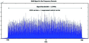
Figure 1. DAB Signal in the Frequency Domain.
3. THE DAB FRAME
When represented in the temporal domain, the DAB signal can be broken down into frames. A frame consists of three main channels, the Synchronisation Channel (SC), the Fast Information Channel (FIC) and the Main Service Channel (MSC) [Reference Palmer, Moore and Hill5]. These are broadcast sequentially in that order with one frame duration being approx 1/10th of a second. Each channel is then broken down into a number of OFDM symbols as shown in Table 1, which are then broken down further to give the DQPSK symbols. Finally, each symbol is broken down into the fundamental unit known as T. T is a unit of time derived from the system clock (2·048 MHz) and may be defined by:
T is used to define the lengths of OFDM symbols in the temporal domain. The symbol lengths of primary importance are shown in Table 2.
Table 1. Symbols in DAB channels.

Table 2. Symbols defined in T.

Each OFDM symbol in the DAB frame is defined as having two distinct portions; the useful symbol and a cyclic prefix or Guard Interval (GI). The GI is a replica of the final 504T of the useful symbol which then precedes the start of the useful symbol making the total OFDM symbol length (see Figure 2). The GI is inserted to allow a buffer for subsequent transmissions from within the network to arrive without interfering with the synchronisation of the first-to-arrive signal. This technique also mitigates Inter-Symbol Interference (ISI). By applying a GI to the front of each symbol, it is possible to use the system as part of a Single Frequency Network as explained earlier.

Figure 2. OFDM+Guard Interval.
4. POSITIONING REQUIREMENTS
4.1. Transmitter Identification Information
The Null symbol is the first symbol in the transmission frame and is used to acquire the rough start of the first OFDM symbol, the Time Frequency Phase Reference (TFPR) Symbol [Reference Layer1], which will be discussed subsequently. In every second transmission frame, the Null symbol contains additional information to allow a receiver to unambiguously identify the transmitters it is receiving on that frequency. This information is broadcast by switching on certain pairs of carriers during this period which are used in two ways. Firstly, the pattern of these carriers allows identification of the Region ID in which the transmitters are operating. Secondly, the position of the carriers within this pattern identifies the transmitter in that region. The pattern switches on four of eight possible carriers and repeats this pattern four times over the width of the signal. This gives a maximum of 70 possible region codes, within which can reside up to 23 possible transmitter codes. This information can be used to cross-reference a database of transmitters which is broadcast as part of the Fast Information Channel and contains location information.
4.2. Time Frequency Phase Reference (TFPR) Symbol
The TFPR symbol forms the second symbol in each DAB frame. The symbol is composed of a Constant Amplitude Zero Autocorrelation Code (CAZAC) waveform, the properties of which allow the receiver to correct the timing offsets caused by the oscillator in the receiver and give the precise differential starting position allowing the first FIC symbol to be decoded. The contents of this symbol are identical in every transmission and are known to the receiver. Therefore, the symbol can be recreated locally and then compared to the received signal. The full details of the TFPR symbol construction are beyond the scope of this paper but are freely available in the ESTI standard [2]. When constructed correctly, the receiver generated TFPR symbol will be as shown in the time and frequency domains (see Figure 3 (Top) and (Centre) respectively). By running the TFPR sequence in the time domain through an auto-correlation function, the result may be seen in Figure 3 (Bottom). This shows that a very clear auto-correlation spike may be attained using the generated TFPR symbol.

Figure 3. Generated TFPR in time domain (Top); in the frequency domain (Centre); and Auto-correlation of TFPR symbol (Bottom).

Figure 4. Sum of signals in time domain (Top); Cross-correlation results (Bottom).
5. CROSS-CORRELATION SIMULATION
This section will examine a combination of these generated symbols in order to simulate multiple signals arriving at the receiver. In this scenario, four signals are generated and the attributes of each differ from each other in three ways. Firstly, following the first signal's arrival, signals two and three have a delay of up to 504T (the length of the Guard Interval). Secondly, the power in each channel will differ due to the transmitter location and differing transmission power. Finally, noise is added to each channel in varying quantities. Using these three parameters, alterations were made to each signal and the values for each are shown in Table 3. Summing all four complex signals from this table gives an absolute signal plot shown in Figure 4 (Top). A cross-correlation of the noiseless generated signal with the four summed signals is then performed. The resulting plot (Figure 4 (Bottom) shows four clear spikes as expected at the precise separation points detailed in Table 3. The relative power of each signal is within 10% of the values given in the table, however the amplitude of the spikes is not really relevant until the identification of individual transmitters (discussed later).
Table 3. Signal properties.

6. TIMING INFORMATION EXTRACTION
It has been shown in the previous section that extraction of timing information is possible using simulated data. This section will now examine the use of this technique with real data. All data in this paper has been captured using the Universal Software Radio Peripheral (USRP) manufactured by Ettus Research LLC. This device was used to capture and store the “raw” frequency data which was then post-processed using Matlab. There are several steps in this process which will now be examined briefly.
6.1. Step 1: Find the Null Symbol
The signal is initially examined in the temporal domain. The first task is to find the first Null symbol as described earlier and therefore the start of the DAB transmission frame. This is done by moving a window over the absolute values of each T point until this falls consistently below a pre-defined threshold. At this point, the window is within the null zone. This process then changes in order to find the end of the current null symbol, again by testing against a threshold. Once found, this point defines the start of the TFPR symbol. This position can be seen clearly in Figure 5. The Null symbol starts from left to right followed by the TFPR and then the first FIC symbol.

Figure 5. Null end position.
6.2. Step 2: Extract the TFPR Symbol
The transmission frame can now be divided up using the symbol length values detailed in Table 2. The TFPR symbol contains 2552T; a Guard Interval (the first 504T) and the useful symbol (the remaining 2048T) are extracted from this. (Figure 6)

Figure 6. First OFDM symbol breakdown.
6.3. Step 3: Remove the signal “fringes”
Following the removal of the GI, the signal is run through an FFT to further process the signal in the frequency domain. The purpose of this is to remove the leading and tailing 256T of the OFDM symbol as this does not contain any useful information. In Figure 1 an OFDM signal is presented in the frequency domain. The useful portion of this is in the range −768T to+768T, the remainder may be removed at this point. The positioning of this window over the useful portion of the signal is paramount here as the next stage involves the cross-correlation with the generated signal as discussed earlier. Receiver clock errors in the USRP must be accounted for before continuing. When the window has been positioned accurately, the remaining signal is then run through an inverse FFT to process the data in the time domain.
6.4. Step 4: Perform the cross-correlation
The signal is now in a state where the cross-correlation can be performed using the previously generated TFPR symbol as shown in the earlier simulation. Figure 7 shows the cross-correlation plot using the local Leicester network. The plot shows the correlation result from one DAB frame but multiple frames may be used for this purpose in order to verify the distance between spikes. The spikes in this plot show a difference of 54T. As a standalone measurement, this merely provides a hyperbola of points at which the receiver may be located. The position estimation process is explained in greater detail in the next section. In order to identify the region and transmitters involved, the Transmitter Identification Information (TII) must also be decoded. As explained previously, this is a two-stage process to identify the pattern (Region ID) and carrier position (Transmitter ID) contained within the Null symbol of every second transmission frame.

Figure 7. Cross-correlation plot using real data.
Figure 8 shows the TII information obtained from the same DAB frame as used in Figure 7. In this scenario, the Region ID can be identified as region 65 which corresponds to the East Midlands (the pattern in this case has the binary value of 1 1 1 0 0 0 0 1). The four taller spikes represent the more powerful transmitter whilst the four shorter spikes are the secondary transmitter. The location of these spikes allows the Transmitter ID to be found; in this case the more powerful transmitter is Copt Oak and the secondary transmitter is Houghton-on-the-Hill. With this information obtained with data from two networks, the estimation of the position of the receiver may be done using TDoA and Least Squares processes.

Figure 8. TII plot using real data.
7. POSITION ESTIMATION
Hyperbolic positioning is used in this process to provide the position estimation based on the TDOA measurements extracted from the DAB data. Figure 9 (Left) shows the theoretical basis upon which this process is performed. Transmitters A1 and A2 form one synchronised pair whilst B1 and B2 the second. Each pair produces one hyperbola of possible TDOA positions (a and b), which will intersect at a point 1. This point is an area of uncertainty, the magnitude of which is dependent on the errors present in the system.

Figure 9. Hyperbolic lateration (Left); TDOA estimation (Right).
Referring to Figure 9 (Right), the position estimation equations can be derived using a partial least squares process. The receiver position R is unknown but can be described as a range to each of the four transmitters. This provides enough information to find R.
8. SIMULATIONS & EARLY RESULTS
Using the techniques described in the sections of this paper, some early results have been obtained and verified using GPS positioning. Before these results are examined, a simulation on the HDOP values present in the test region is presented. The simulation takes into account the locations of the four transmitters. The HDOP values are calculated using the two pairs of transmitters. Figure 10 shows the results of this simulation; the blue regions indicate the lowest HDOP whilst the red regions indicate the highest, up to a maximum value of 50. The networks used for these results were the Leicester local and the Nottingham local due to the fact that they use different transmitter sites, making the verification of received transmitters simpler for the early testing. Extracting the TII data and tracing the two plots on the same set of axes, it is proven that we have the IDs for four transmitters. Using the location of the spikes, we can identify each transmitter using information freely available from the Office of Communication (OFCOM) website [6]. Figure 11 shows this result. Knowing that we have four transmitters with which to perform the location estimation, the process continues and cross-correlation spikes are found for both networks (Figure 12).

Figure 10. HDOP in test region.

Figure 11. TII for Nottingham & Leicester networks.
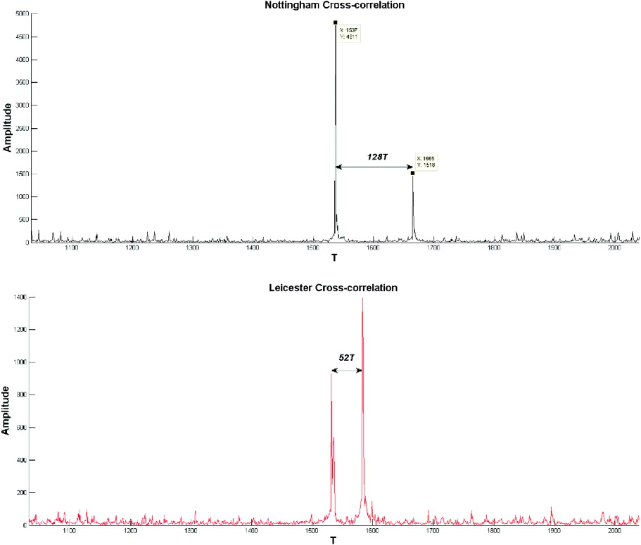
Figure 12. Nottingham network cross-correlation (Top) and Leicester network cross-correlation (Bottom).
These measurements allow us to establish a position estimate, however we have not yet accounted for the timing biases inserted by the operators of each single frequency network. These are not always present but can be inserted to ensure that signals in each network do not arrive outside of the guard interval, so as to avoid inter-symbol interference. To account for this, measurements from two reference locations must be made to find the offset (if any) from each transmitter. Each reference location requires a measurement taken by a GPS receiver to establish the known position. With two such measurements, the potential biases for all four transmitters may be accounted for.
Transmission biases have to be corrected in this way each time a new transmitter is detected. The biases are also dependent on each network, not each transmitter (i.e. Multiple networks using the same transmitter may have different biases due to the geometry/transmission power of each transmitter in the network).
The plot in Figure 13 is included to show the test area including all transmitters. It indicates the positions of the four transmitters by blue triangles and the cluster of points to the top left is the test area. This has been enhanced in Figure 14 to show the deviation of GPS locations (indicated by red crosses) to the DAB standalone calculation (indicated by black crosses – difference indicated by the adjoining lines).

Figure 13. Test area and transmitters.

Figure 14. Initial results.
The measurements made using the DAB positioning software point towards a mean error of just over 150 m with a maximum error of 290 m and a minimum of 60 m (see Figure 15). The mean error figure is the figure expected due to the limiting factor of the sampling unit T which corresponds to approximately 146 m. A sub-T resolution should be possible if the hardware front-end is capable of over-sampling the captured signal. The USRP front-end used in this case is not capable of doing this. A follow-on project is intended to investigate measurements of a higher resolution.

Figure 15. Positioning offsets.
9. CONCLUSIONS
The early results presented in this paper indicate that a stand-alone positioning system using multiple DAB networks is possible but will be area dependent. It is in difficult GPS reception areas, such as indoors or urban canyons (in highly populated areas) when GPS is unavailable or of very poor quality, where this system could show its strength, as has been shown using the DVB signal in [7]. Less populated areas will naturally have fewer transmitters and therefore less chance of providing sufficient information to establish a position estimate. However, the GPS signal would naturally be more prominent in these cases. In many regions, different networks will use the best (and therefore same) transmitter sites. To overcome this constraint, a combination of two or more local SFNs can be used for timing measurement purposes.
There are a number of possible error sources that need to be investigated in order to establish the true robustness of the algorithms involved:
• The broadcast transmitter locations have not been precisely surveyed (due to access constraints) and it is estimated that the measurements are within 100 m of their true locations. This would account for a large error.
• In the two networks used for this working example, the TII information indicates that only two transmitters are being received for each. However, a third much weaker transmitter could present problems when tracking the correlation spikes.
• A timing delay bias could be present on one or both networks. This would be deliberate as part of the design of the Single Frequency Network in order to avoid inter-symbol interference. Provided a measurement can be taken from a known location, all received transmitter biases may be mitigated simultaneously.
• The geometry of the transmitters relative to the receiver currently places the receiver in an area of poor geometry. This could explain the poor precision as the location would naturally have a higher HDOP [Reference Palmer, Moore and Hill5].
• Smaller errors could involve the relative heights of the transmitters and receiver, different transmission powers and the terrain of the test region.
10. FUTURE WORK
As mentioned previously, the system described in this paper is effectively limited by the sampling rate of the transmitted signal (146 m accuracy). The use of hardware with the capability of over-sampling the signal would allow an early/late type correlator to be used in a similar way to a GPS receiver. This should achieve a resolution better than the timing unit T.
The signals are currently captured in their raw state for the purpose of post-processing. This data fills a large amount of storage space, depending on the length of the capture (~15 MB/sec/network). Each network only requires a frame or two to calculate a position, however this makes the current set-up inappropriate for continuous tracking. Integration of a new front-end with a real-time SDR system would achieve an accurate and robust positioning system without the need for large quantities of storage.