2. The Data

2.1 The Financial Times-Actuaries Share Indices, now the FTSE Actuaries Share Indices, commenced in April 1962, and included an index of Earnings Yields for what at that time was called the “500 Index”, now the Non-Financial Index (NFI). In July 1965 there was a change to publishing P/E Ratios, and in December 1992 P/E ratios and Cover (i.e. Earnings/Dividends) were published for the All-Share Index (ASI) as well. Thus, there are two possible indices to be considered. Over the time there have also been changes in the taxation of the earnings of companies and in the taxation of dividend income for investors. So there are several points to be considered before we have a straightforward set of indices for statistical analysis.

2.2 By 1962 most UK companies had been required to publish “true and fair” consolidated earnings for the entire group, rather than the artificial accounting earnings produced previously for the top company in any group. So it was worth producing an index of share earnings. However, this requirement did not apply to financial companies. An index of Earnings Yields (i.e. Earnings/Price as a percentage) was published in the Indices for the “500 Index”, an index of all companies except financial ones. A change of taxation suggested changing to publishing P/E ratios (i.e. 100/Earnings yield) from July 1965 onwards.

2.3 By 1992 financial companies had also been required to publish true and fair consolidated earnings, so P/E ratios, and also an index of Cover (i.e. Earnings/Dividends) could be published for all sectors of the indices including the ASI. We have not considered the individual industrial and financial sector indices (although these would repay separate investigation), but only the Non-Financial and the All-Share ones. Given the Price Index, Dividend Yield, and P/E Ratio, we can calculate implied Earnings Indices and implied Dividend Indices. We would prefer to use the All-Share one, as representing the full stock market, but in order to go back to 1962 we need to use also the NFI. So we splice them together in a way described in section 2.7.

2.4 First, however, we must consider how taxation affects these indices, since “earnings” are determined after corporation tax has been paid. The method of taxing companies has changed over the years. A new system was introduced in 1965, which justified the change in the indices from Earnings Yield to P/E Ratio. For some years the rate of company taxation had depended on how much of the profit was paid out in dividends and how much was retained. This meant that the earnings yield depended on the dividends. It could be defined in three ways, two extreme ones assuming either maximum dividends or no dividends, and the third assuming the actual payouts; this third was used for the indices. This also meant that “cover” could have alternative definitions. We have used the published figures throughout. We should note that the rate of corporation tax has reduced from over 50% in 1965 to 20% currently (2016), with more reductions possible. This alone could have increased earnings net of taxation by over 60%, or around 1% per year over the period. This should be noted when considering the real rate of growth of earnings.

2.5 The rate of taxation on dividend income has also changed over the years, and varies considerably depending on the tax status of the recipient. For a long period the income of UK pension funds and of the pensions business of UK life insurance companies was free of income tax, and a “gross yield” was therefore appropriate for many actuarial purposes, and this was used for the indices. But this system was changed in 1999; the actual dividends paid carried a 10% notional tax credit, which, however, was not repayable to any UK investors, but counted for taxable investors as if 20% tax had been paid. The indices changed to publishing an “actual dividend yield”, which excluded the 10% credit. In our previous calculations in the Parts of this series we have grossed this up by dividing by 0.9, to give a gross equivalent yield which seemed more compatible with previous amounts, while noting that our figures should be multiplied by 0.9 to get back to the present published values. But it now seems appropriate to use the actual figures unadjusted, since we are now looking at the position of the company, and comparing the actual cost to the company of their dividend payments with their published earnings.

2.6 The three ratios that can be calculated for these indices are: P/E Ratio, Dividend Yield and Cover. Given any two the third is determined. We also have a Price Index, a Dividend Index, and an Earnings Index. For the NFI these all exist from April 1962. For the ASI the earnings series exist only from December 1992. We wish to splice the two series together, using the ASI for the later period and, necessarily, the NFI for the earlier one. Inspection shows that at the end of March 1994, 15 months after the ASI Earnings series started, the Dividend Yields for the two series (which are given to two decimal places) were the same at 3.72%, and the P/E Ratios were close at 20.60 for the ASI and 20.54 for the NFI. This seems, therefore, a suitable date to join the series. A formal test can be carried out, calculating, at each date:

$$\left( {{{DY_{{{\rm ASI}}} } \over {DY_{{{\rm NFI}}} }}{\minus}1} \right)^{2} {\plus}{\rm }\left( {{{PER_{{{\rm ASI}}} } \over {PER_{{{\rm NFI}}} }}{\minus}1} \right)^{2} $$

and we find that this value is minimised at 0.0009 in March 1994. If we did not choose a date when the relevant values were close, and chain linked the price indices, there would be undesirable jumps in the dividend and earnings indices.

2.7 We therefore calculate a Composite Index, using the ASI figures from March 1994 onwards, the NFI figures for Dividend Yield and P/E Ratio up to February 1994, and multiplying the Price Index values for the NFI by Price Index _ASI/Price Index _NFI at March 1994. We then calculate a Dividend Index and an Earnings Index for the Composite Index from these figures.

2.8 We can compare the Dividend Yield for the two indices. Up to March 1994 they were within 10% of each other, and in a graph they are almost indistinguishable. If we plot the Price and Dividend Indices on the same scale, they too are almost indistinguishable. This is not surprising, since the NFI forms a very large part of the ASI. A full series of the market values of the stocks in the two sectors is not available, but we can estimate that the Financial Sector has been perhaps 20%–30% of the total. Since March 1994 there has been greater divergence in the Dividend Yield and P/E Ratios with variations up to 25% or so. The financial crisis of the late 2000s caused certain large banks to show much reduced earnings and dividends reduced to zero, this causing the divergence. But we prefer to use the largest market that we can, so do not avoid these features.

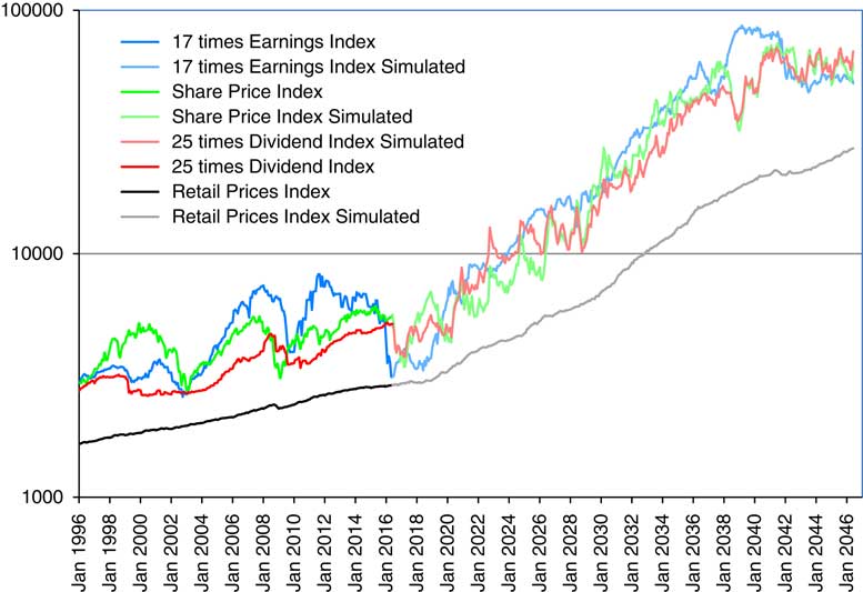
2.9 In Figure 1 we show the Composite Price Index, 25 times the Composite Dividend Index, and 17 times the Composite Earnings Index, as well as the Retail Prices Index (RPI), all scaled to fit into two cycles of a vertical logarithmic scale. Observe that the RPI is much the most stable of the four, with the Dividend Index next, the Earnings Index fluctuating more, and the Share Price Index fluctuating yet more.

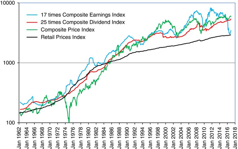
Figure 1 Retail Prices Index and Composite Price Index, 25 times Dividend Index and 17 times Earnings Index. April 1962 to June 2016.

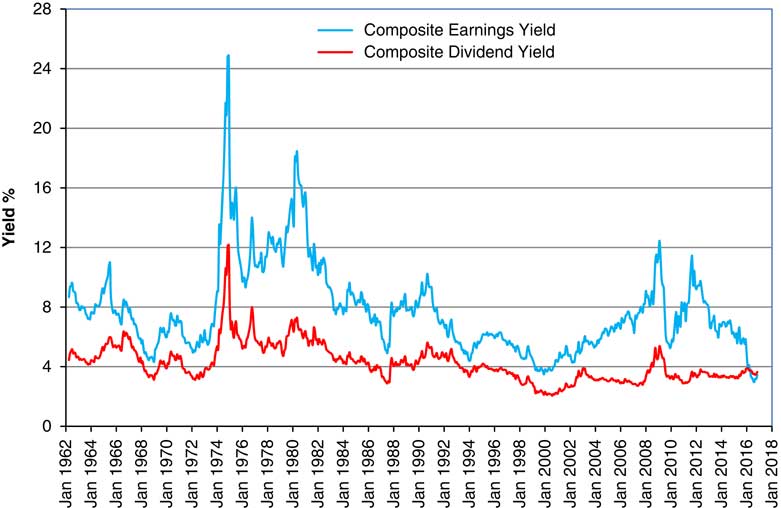
2.10 In Figure 2 we show the Dividend Yield and the Earnings Yield (calculated as 100/P/E Ratio) for the Composite Index. Observe how they tend to go up and down together as share prices change. Note also that up to the end of February 2016 the Earnings Yield was always above the Dividend Yield, so the Cover, which is the ratio of these, was always greater than unity. However, in February 2016 Cover on the ASI fell to 1.00 and on the NFI to 0.78, indicating that non-financial companies in aggregate were dipping into past reserves to pay dividends. In May 2016 there were further big falls in Cover for both indices, to 0.89 and 0.67, with almost no change in June 2016. Several very large companies in the mining and oil sectors published losses, so for certain sectors published P/E Ratios and published Cover were negative. It is not clear how one could easily model negatives here, when we generally wish to work with the logarithms of earnings, so in this paper we ignore the possibility of negative earnings on the whole index, though we recognise that this is not an impossibility.

Figure 2 Earnings Yield and Dividend Yield for Composite Index.

2.11 In subsequent analysis we use data from June to June and we observe a very severe drop in the share earnings index from June 2015 to June 2016, of just over 50%, or in log terms of −0.7245. This is over 2.5 times the next largest decrease (in 1965–1966) and almost twice (in absolute terms) the largest increase (in 1973–1974). Over the same period Cover fell by a little more, from 1.91 to 0.89, a drop in Ln(V(t)) of −0.7645. These are therefore both outliers, and it is worth investigating also the period up to 2015 to see what difference they make.

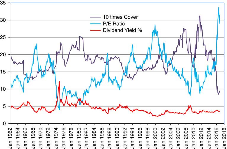
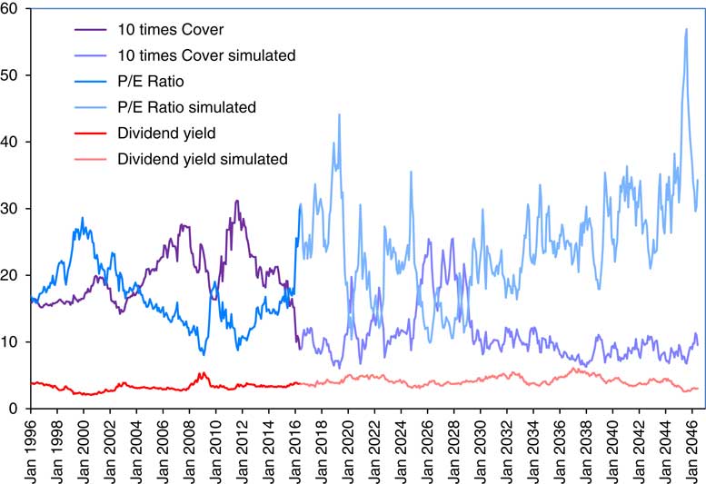
2.12 In Figure 3 we show the Dividend Yield along with the more familiar ratios, Cover (multiplied by 10 to fit into the scale better) and P/E Ratio. We see the P/E Ratio reaching a peak at the height of the “dot com” bubble at the end of 1999, but going higher than that during 2016. We see Cover going below 1.0 in the same period, having reached a peak of more than 3.0 in September 2011.

Figure 3 Dividend Yield, 10 times Cover and Price/Earnings (P/E) Ratio, for Composite Index.

3. Approaches

3.1 In the original model Wilkie (Reference Wilkie1986) modelled share dividends, D, and dividend yields, Y, the ratio giving the share price, P=D/Y. However, we consider that earnings are more fundamental. For most companies their earnings depend on trading profits, although there are a few exceptions, like investment trusts, whose income comes from the dividends of other companies in which they have invested. It is on the basis of earnings that company directors decide or recommend dividends, and it is on the basis of earnings and dividends, both past and prospective, that investors base the price of shares. These in turn depend on current and past inflation, so a model like that used previously for dividends might be appropriate for earnings.

3.2 The original annual model for dividends was based on the annual change in the logarithm of the dividend index, with K(t)=DL(t)−DL(t−1), where DL(t)=LnD(t) and D(t) is the value of the dividend index at time t, and t is measured in years. We can denote the earnings index at time t as E(t) (noting that Wilkie, Reference Wilkie1995 used E for property earnings, but in this context there is no confusion). We then put EL(t)=LnE(t) and then L(t)=EL(t)−EL(t−1). We also denote the share prices index as P(t), with PL(t)=Ln(P(t)) and PLD(t)=PL(t)−PL(t−1), but we do not model it directly.

3.3 We have three interconnected ratio series, Dividend Yield, P/E Ratio, and Cover, and we need to model only two of them. Their product is always 1 (or 100 if we use percentage yield). Each of the ratio series is apparently autoregressive in some way, stationary around some central level, but not extremely high or extremely low; and all must be positive (at least we assume so). But there seem to be three possible routes. One is to model Cover, giving a Dividend Index, and then Dividend Yield to give a Price Index. This leaves the P/E Ratio as a derived series, calculated from Prices and Earnings; yet it is an item that investors pay much attention to. A second route is to model the P/E Ratio, giving a derived Price index, and then Cover to give a Dividend Index. That leaves Dividend Yield as a derived series. The third route is to model the P/E Ratio, giving a Price Index, then Dividend Yield to give a Dividend Index. In this case Cover is the derived series. We choose the first of these possibilities, modelling Cover and Dividend Yield, but keeping in mind that the P/E Ratio may be relevant.

3.4 Another approach would be to consider Earnings, Prices, and Dividends directly, perhaps with a co-integration model. It is reasonable to assume that investors look at both earnings and dividends when assessing the value of a company. But if, for example, a company chooses to keep its cover roughly constant at about 2, it is impossible to determine whether a particular price is 20 times the dividend, or ten times the earnings. A model like this would fail as being indeterminate.

3.5 It is natural to take logarithms of the three main series, Earnings, Dividends, and Prices, and also of Dividend Yields, Cover, and P/E Ratios in order to keep them positive. Cover, which we denote V(t), is a special case. In general, a company can only pay out dividends from current earnings or from previously undistributed earnings. So in the long run, the Payout Ratio (equals 1/Cover) cannot be greater than unity, or Cover less than unity, although in particular years this is quite possible, and it is not infrequent if a company has a temporary setback. We originally considered modelling VL(t)=Ln(V(t)−1), since the lowest observed value of Cover in our composite series up to June 2015 was 1.28 (in December 1967 and again in February 1994) but as noted above Cover on the ASI has dropped to 0.89 (and that on the NFI to 0.67), showing that it would be possible for the whole economy to be such that companies in aggregate have uncovered dividends. So we did not follow this original possibility. We reject modelling V(t), unlogged, because its possible range is the whole real line, and negative Cover is not appropriate, since we assume that at least earnings on the whole index remain positive, and dividends are necessarily non-negative. So we model the logarithms of earnings and of dividends, keeping them both positive, and thus excluding negative cover.

3.6 In accordance with our previous analyses we shall look first at the annual data, using, as before, the June values. But it is worth considering what the results would be if we used other months, which we may consider in a later paper. Since we have monthly values we can also look at them either as a monthly series or as intermediate values for stochastic interpolation.

3.7 It is worth while considering what relationships between these variables we might expect, based on economic and investment principles. If retail prices rise it is reasonable to expect company sales to rise too, but also for wages to rise. The net effect, other things being equal, would be for company earnings to increase roughly in line with prices. But whether this is best expressed in the way we have modelled wages, with an effect in two successive years, or in the way we have modelled dividends, with an exponentially weighted moving average of past inflation plus a simultaneous effect, is something that needs to be investigated.

3.8 Earnings may also be affected by wages, over and above the change in retail prices. There are two possible and contradictory effects here. If the economy is doing well, then wages and company earnings may rise together, and likewise they may fall together if the economy is doing badly. But there is also tension between the two in the old conflict between Labour and Capital, so that at times wages may rise at the expense of earnings, and at other times the position may be reversed. The first effect would suggest a positive correlation, the second a negative one, between the two indices. This is a matter for investigation. However, many companies now in the UK indices operate very much outside the United Kingdom, so any connection with Wages in the United Kingdom may be small.

3.9 We then expect dividends to rise with company earnings, but perhaps with a lag, and share prices to rise too, but possibly in anticipation. Those in the investment market know well what the economy has been doing, and may have their own estimates of next year’s company earnings, based also on any announcements from individual companies. Remember that the earnings of a company for one trading year are not exactly known until after the year has finished, and are not announced immediately, so there is plenty of time for share prices to anticipate company earnings reasonably well. We reflected this in the dividend model with a term relating dividends to past yield changes, DY.YE(t−1). It might be reasonable to expect a similar anticipatory effect for earnings.

3.10 If earnings are higher than the model expects, then it is only to be expected that cover also increases, unless dividends are increased pari passu. But it is more likely that directors attempt to smooth out changes in earnings, not increasing dividends too quickly, and not reducing them immediately if company earnings decrease, even to a loss. So we would expect a positive relationship between simultaneous changes in cover and earnings.

3.11 All this suggests possible relationships that we might expect when we come to investigate the data. If some statistical relationship is observed, perhaps with only marginal significance, we would prefer to include it in the model if it represents a plausible economic or investment effect, but we are less inclined to include it if there seems to be no rationale to explain it. This is necessarily a little subjective, but we believe not unreasonable, and we document our decisions so that others may take a different view.

3.12 Little (Reference Little1962) and Little & Rayner (Reference Little and Rayner1966) investigated the growth of the earnings of individual UK companies over the 1950s, and postulated a hypothesis of “higgledy-piggledy growth”, in effect a random walk for company earnings. They did not have a long run of data and did not have an overall index. We have used a different, and much longer period, and the overall index, rather than individual companies, but, as we shall show, come to much the same conclusion.

4. Initial Data Analysis

4.1 We now have data for a mixture of periods. Our older series of Retail Prices is available as before from 1923, our usual starting date. Our original series for Dividend Yields and Dividends are also available from 1923. Our newer series, for Share Earnings, Cover, and P/E Ratios are available only from April 1962. And we now have a second series for Dividend Yields and Dividends, based on the composite share index. In our earlier papers we have adjusted the quoted “Actual Dividend Yield” since April 1999, grossing it up by dividing it by 0.9, noting that adjustments needed to be made to accord with the current published figures. However, we now use the actual yield unadjusted in all our calculations, so that our results can be used directly.

4.2 We have previously used June figures to get annual series, and we do the same now, noting, however, that it might be of interest to investigate what the results would be if we should use other months. We have all the series up to June 2016, so we can end our series in that month.

4.3 For the time being we shall use our older Retail Price Index Series, refitting it, however, over the period from June 1923 to June 2016. Then we shall use the new, composite, share series, Earnings, Cover, and Dividend Yield, from June 1962 to June 2016, reverting also to the original older Dividend Yield and Dividend series for comparison.

4.4 We can start by giving the basic statistics for the different series, the means and standard deviations (s.d.s), not allowing for any auto- or cross-correlations. We use the differences of the logarithms for the non-stationary series, as

$$\eqalignno{ &\hskip -55pt {\rm Retail}\,{\rm Prices\,\colon\,}\,Q\left( t \right)\,\colon\,\,I\left( t \right)\, {\equals}\, QLD\left( t \right)\, {\equals}\, {\rm Ln}Q\left( t \right){\minus}{\rm Ln}Q\left( {t-1} \right) \cr {\rm Share}\,{\rm dividends}\,&\colon\,\,D\left( t \right)\,\colon\,\,K\left( t \right)\, {\equals}\, DLD\left( t \right)\, {\equals}\, {\rm Ln}D\left( t \right){\minus}{\rm Ln}D\left( {t-1} \right) \cr {\rm Share}\,{\rm earnings}\,& \colon\,\,E\left( t \right)\,\colon\,\,L\left( t \right)\, {\equals}\, ELD\left( t \right)\, {\equals}\, {\rm Ln}E\left( t \right){\minus}{\rm Ln}E\left( {t-1} \right) \cr {\rm Share}\,{\rm prices}\,&\colon\,\,P\left( t \right)\,\colon\,\,PLD\left( t \right)\, {\equals}\, {\rm Ln}P\left( t \right){\minus}{\rm Ln}P\left( {t-1} \right) $$

4.5 For the series that we expect to be stationary we use the logarithms:

$$\eqalignno{ {\rm Dividend}\,{\rm Yield}\,&\colon\,\,Y\left( t \right)\!\!:\,YL\left( t \right)\!\!:\, {\equals}\, {\rm Ln}Y\left( t \right) \cr {\rm Cover}\,&\colon\, V\left( t \right)\!\!:\,VL\left( t \right)\!\!:\, {\equals}\, {\rm Ln}V\left( t \right) \cr {\rm P\!/\!E}\,{\rm Ratio}\,&\colon\,\,M\left( t \right)\!\!:\,ML\left( t \right)\!\!:\, {\equals}\, {\rm Ln}M\left( t \right) $$

4.6 In Table 1 we show the basic statistics for the different series and for different periods, at this stage ignoring auto-correlations and other dependencies. Note that we have values for earlier years for the series that we start in 1923, so we know I(1923), K(1923), etc. But for Dividends and Earnings, commencing in 1962, we do not have the differences, K and L until 1963, so we start then. When we later include regression on earlier values in our analysis we have to start Cover and Dividend Yield a year later too, so we show values for them from 1963.

Table 1 Basic statistics of series used.

4.7 We can observe that the mean for K, Dividends, is higher than that for I, Retail Prices, over both the longer and the shorter periods. However the mean for L, Earnings, over the shorter period to 2016, is slightly less than that of I. We can also observe that the standard deviation for L is much higher than that for K, which in turn is higher than that for I, which is similar over the two periods. The means of the stationary ratio series, all logged, would not be easy to interpret, so we quote the exponents of the means. The standard deviations are comparable, and are all quite large compared with the basic series.

4.8 Comparing the numbers in Table 1 for Earnings and Cover ending in 2016 with those ending in 2015, we see that the mean rate of growth of Earnings has been reduced by about 1.5% a year, and the s.d. has risen from 0.1545 to 0.1864, by more than 0.03. The mean of Cover is affected less, but the s.d. is also increased by about 0.02.

4.9 We show also the skewness and kurtosis for each variable. While some variables, like YL in both periods, show values of these close to 0.0 and 3.0, so can be assumed to be normally distributed, others show quite high values of both statistics, indicating non-normality, usually with fat tails. Similar features appear in the residuals after fitting the models, as we show below. However, we postpone discussion of possible alternative distributions to a later part of this series.

4.10 We calculate the auto-correlation and cross-correlation coefficients of all the series, and we observe, as we would expect, that there is strong auto-correlation in every case, and in many cases strong cross-correlation with Retail Prices, and with other series. These are all interconnected, and the modelling attempts to unravel them.

5. Retail Prices

5.1 We simply update the existing models for Retail Prices and Wages, using the latest data up to 2016, and we expect quite small changes from our update in 2009 (Part 1). However, we also observed a notable correlation between the residuals of I(t) and J(t−1) (i.e. the change in Wages in the previous year), which our model had not previously paid attention to, and which we hope to investigate in a subsequent Part of this series.

5.2 The original model for I(t) is a simple autoregressive model of order one (AR(1)), which we express as

$$\eqalignno{ & IN\left( t \right)\, {\equals}\, QA.IN\left( {t-1} \right){\plus}QSD.QZ\left( t \right) \cr & I\left( t \right)\, {\equals}\, QMU{\plus}IN\left( t \right) \cr & QL\left( t \right)\, {\equals}\, Q\left( {t-1} \right){\plus}I\left( t \right) \cr & Q\left( t \right)\, {\equals}\, {\rm exp}\left( {QL\left( t \right)} \right) $$

We fit over the periods 1923–2016 and 1963–2016, and show the results in Table 2, including also the results obtained in Part 1 for the period from 1923 to 2009.

Table 2 Results for Retail Prices.

5.3 We show the estimated parameters, and also their standard errors (s.e.s). We estimate parameter values, as always, by maximising the log likelihood, and in doing this assume that the residuals are normally distributed. But we also show the Skewness and Kurtosis coefficients and their Jarque–Bera (JB) probability. For all periods the Kurtosis is very large (for a normal distribution it would be 3.0) and the Skewness is also large (for a normal distribution it would be zero), so the Jarque–Bera probability is negligible. This observation is not new, but it does mean that the true standard errors of the statistics may be higher than we show. We do not investigate alternative distributions for residuals here, but we hope to do so in a later Part of this series.

5.4 The results we obtained ending in 2009 are quite close to those in 2016. Over the shorter period starting in 1963 the values of QA and QMU are higher, but not by much more than about 1 s.e.

5.5 For certain comparisons for subsequent series investigated over the period 1963–2016 we use the model for I(t) fitted over the same period; but in general we prefer the model fitted over the longer period.

6. Dividend Yield

6.1 We present first the model for Dividend Yield, Y(t), in the same form as has been used since the start of these investigations. We put it before Earnings, because we find a small lagged effect of Yield on Earnings, as we did for Dividends. A natural way of looking at all these series would be with a full vector autoregressive (VAR) model, where every series has an opportunity to influence every other series at a later date. However (apart from our observation in section 5.1), we have always found that a “cascade model” is satisfactory; it is easier to model, and to construct and, we think, easier to understand than a full VAR one. At each step we look for possible lagged correlations, and reorganise the ordering of our series to account for these. We present the series as finally modelled, so Dividend Yield comes in sequence here.

6.2 The model for Y(t) puts YL(t)=Ln(Y(t)), and YMUL=Ln(YMU), and is then

$$\eqalignno{ & YN\left( t \right)\, {\equals}\, YA.YN\left( {t-1} \right){\plus}YSD.YZ\left( t \right) \cr & YL\left( t \right)\, {\equals}\, YMUL{\plus}YW.I\left( t \right){\plus}YN\left( t \right) $$

6.3 We have now, rather confusingly, three series for Y(t), one that we have used until now, that dates back to 1920 and since April 1992 uses the “actual yield” grossed up by dividing it by 0.9, which we call the “Adjusted” series; the second the same, but not adjusting the actual yield, which we call the “Unadjusted” series; the third the “Composite” dividend yield described in section 2, based on the NFI figures from 1962 until 1994 and the ASI figures thereafter, with the actual yield not grossed up. For compatibility with our previous calculations we have updated the former two series to 2016, and show the results in the left-hand part of Table 3. The parameter values are quite close to each other, and close to those based on the Adjusted series to 2009, as in Part 1, and shown in the next column.

Table 3 Results for Dividend Yield.

6.4 We estimate the parameters for the Composite Index for the period 1963–2016 using the usual model, and show the results in Table 3. Although the basic yield series shows quite a high value of skewness and a very high value of kurtosis, the residuals become more like normally distributed after the connection with inflation is introduced.

6.5 We also show the results for the Unadjusted series from 1963 to 2016. The two series have reasonably similar values of the parameters, and these are not very different from those for the longer periods. To be consistent with our other new calculations, we use the parameter values for the Composite Index for 1963–2016 for further calculations in this paper. But in general we prefer to use the parameters for the Unadjusted series for the longer period.

7. Share Earnings

7.1 We next model Share Earnings. Our first thoughts were that the Share Earnings Index, E(t), might require a model similar to Share Dividends, in which the primary component is an exponentially weighted average of past inflation. But experiments soon showed that this was unnecessary, since the rates of inflation only in the current and previous years were relevant, and these, perhaps surprisingly, in opposite directions. Further investigations showed a significant correlation with the residual of the Dividend Yield series in the previous year, YE(t−1), as we suspected might be the case, since it appears in the original Dividend model. There were other connections between the values of E(t) and the values or residuals of other series, but simultaneous ones, which we represent in the models for the other series.

7.2 We model the annual change in the logarithm of E(t), L(t), and show our results in Table 4 in successive steps, with Step 0 the naïve one, where the only parameters are the mean and standard deviation of the successive values of L(t) for the 54 years from 1962–1963 to 2015–2016, so that

$$\eqalignno{ & L\left( t \right)\, {\equals}\, EMU{\plus}ESD.EZ\left( t \right) \cr & EL\left( t \right)\, {\equals}\, EL\left( {t-1} \right){\plus}L\left( t \right) $$

Table 4 Results for Share Earnings.

The skewness and kurtosis are large and not consistent with the residuals being normally distributed; this has arisen mainly from the very large drop in Earnings in 2015–2016. If we omit this last year, they are fairly normal. Inspection of the auto- and cross-correlations of the residuals shows quite strong simultaneous and rather weak lagged correlation with inflation, and little correlation with the Wages series, but a strong lagged correlation on Dividend Yield.

7.3 In Step 1, we introduce the expected connection between the change in Earnings and the current year’s inflation, I(t), so the formula becomes

$$L\left( t \right)\, {\equals}\, EMU{\plus}EQ1.I\left( t \right){\plus}ESD.EZ\left( t \right)$$

but the coefficient, EQ1, has a value of 1.5166, showing an effect of inflation of greater than one for one. The mean, EMU, drops to less than zero, showing no additional real growth in earnings. There is a small negative correlation with inflation in the previous year, so we introduce this next.

7.4 In Step 2, we include a term relating to inflation in the previous year, I(t−1), so the formula becomes

$$L\left( t \right)\, {\equals}\, EMU{\plus}EQ1.I\left( t \right){\plus}EQ2.I\left( {t-1} \right){\plus}ESD.EZ\left( t \right)$$

The estimated value of EQ1 goes up to 2.5561 and that of EQ2 comes in at −1.5192. The combination, EQ1+EQ2, equals 1.0369, so the combination shows close to a one for one effect of inflation. It is therefore worth trying Step 3 with EQ2=1−EQ1. We get EQ1 equal to 2.5380 and EQ2 equal to −1.5380. The log likelihood is hardly changed, and the new values of both parameters are well within the confidence intervals from Step 2, so we prefer this formula.

7.5 We now bring in the correlation with the Yield residual in the previous year, YE(t−1), giving Step 4:

$$L\left( t \right)\, {\equals}\, EMU{\plus}EQ1.I\left( t \right){\plus}(1{\minus}EQ1).I\left( {t-1} \right){\plus}EY.YE\left( {t-1} \right){\plus}ESD.EZ\left( t \right)$$

The improvement in log likelihood is substantial (4.40), and the value of EY significant, just over three times its standard error. As expected, it is negative, indicating that “the market” is able to forecast short-term changes in earnings, so prices rise and yields go down if earnings are expected to rise. At each step the increase in log likelihood is significant, but not very large. The value of ESD is reduced, but not enormously, equivalent to an R ² in a multiple regression of about 0.34. The standard errors of EMU are relatively large, so that the value of EMU is not significantly different from 0; in effect, we cannot get a good estimate of the value of EMU, because the variation is so great.

7.6 We also fit our final model to the Earnings series up to 2015 (leaving other models unchanged). The results are shown in the rightmost column of Table 4. Many of the parameters are little changed, but the estimated value of EMU goes up from −0.0041 to +0.0099, showing that over this period Earnings rose about 1% a year more than Retail Prices. However, the standard error of EMU, at 0.0157, is still large. The standard deviation, ESD, over the shorter period is much smaller, but it would have been so with any of the models.

7.7 The effective mean increase in Earnings, which we can call EMU*, can be calculated as EMU*=EMU+(EQ1+EQ2)×QMU=EMU+QMU. This is shown in the bottom row of Table 4, assuming that the value of QMU is 0.0533, the value estimated for 1963–2016. We see that Earnings have decreased relative to inflation over the period ending in 2016, and we noted in section 2.4 that the reduction in the rate of corporation tax over the period was equivalent to an increase in earnings of about 1%, so the effective rate of increase in real earnings appears to be well below zero. But our end-point shows such a large fall in earnings over a single year that this may well not be representative of a longer future period.

7.8 The skewness and kurtosis of the residuals are also shown in Table 4, and are very large, not at all consistent with normality. But this is greatly affected by the experience of the final year, because up to 2015 the residuals seem to be reasonably normal.

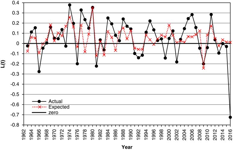
7.9 In Figure 4 we show the Actual values of the change in log Earnings, L(t), from 1963 to 2016, along with the “Expected” values, that is, the expected according to the model. It can be seen that the expected often moves in the right direction, but often not so far, and sometimes too far. However, we should note that the “Expected” values here are not those conditional on the facts known at time t, ℱ _t , but depend also on knowing the value of I(t) already. We discuss forecasts conditional only on ℱ _t in section 13.

Figure 4 Actual and expected values of change in log Earnings, L(t), 1963–2016.

7.10 It may seem curious that the effect of inflation on Earnings is large and positive in the current year, and quite large but negative in the following year. One might rationalise this by saying that a rise in retail prices immediately affects a company’s sales income, without immediately affecting its expenses, so that it has a geared effect on earnings. But a later response may be that employees get higher wages, input prices rise and interest costs increase if interest rates go up, so earnings in the following year can be affected negatively. The overall effect is close to one for one, which we make exactly so. However, this is an explanation for a simple manufacturing or trading company and companies vary considerably. We have no evidence to support this rationalisation; it is a matter for econometricians, and our interest is in financial markets. Indeed in our data, there is no evidence of significant correlation between changes in Earnings and changes in Wages, nor in changes in Interest Rates.

7.11 We discuss other aspects of the model for Earnings in sections 12 et seqq.

8. Cover

8.1 We model Cover, V(t), for the period from June 1962 to June 2016, giving 55 yearly observations, but because of the auto-correlation we use only the last 54, while including the value for 1962 in the calculations for 1963. Step 0 brings in the mean VMUL=Ln(VMU) and standard deviation VSD, and the estimates for these are as shown in Table 1. We could use VMUL directly as the parameter, but there seems an advantage in putting VMU as a more natural mean, as we do for the Dividend Yield model.

8.2 We then observe several high correlations, one the autocorrelation between the residuals for Step 0, with a first autocorrelation coefficient of 0.5938; then a correlation with the residual of the Earnings series EE(t) of 0.5455, then a correlation with the rate of inflation in the year, I(t), of 0.3156. We bring all in these in successive steps, with also an extra term, involving the previous year’s earnings residual, EE(t−1). We might also expect a negative correlation with Dividend Yield, since VL(t)=EL(t)−DL(t) and YL(t)=DL(t)−PL(t), so DL(t) enters both formulae with opposite signs; this is not apparent at Step 0, but does prove significant later on, both simultaneously and lagged 1 year.

8.3 Investigation of all these options gives us a model:

$$\eqalignno{ & VN\left( t \right)\, {\equals}\, VA.VN\left( {t-1} \right){\plus}VE1.EE\left( t \right){\plus}VE2.EE\left( {t-1} \right){\plus}VY1.YE\left( t \right){\plus}VY2.YE\left( {t-1} \right){\plus}VSD.VZ\left( t \right) \cr & VL\left( t \right)\, {\equals}\, VMUL{\plus}VW.I\left( t \right){\plus}VN\left( t \right) $$

We considered also a term in VN(t) of VQ.QE(t) rather than the YW.I(t) term in VL(t). This involves a correlation with the residual, rather than the value, of the Retail Prices series, but it was less effective than what we have put, so we omit it.

8.4 We show the results of successive steps in Table 5. Successive steps all bring a large increase in the log likelihood; the smallest is for Step 5 at 4.41. The estimated values of the parameters are several times their estimated standard errors, so are all fully justified. The standard deviation, VSD, is also greatly reduced, equivalent to a large R ² of 0.93.

Table 5 Results for Cover.

8.5 The skewness and kurtosis vary considerably, but with the final step are quite reasonable, so we might accept the assumption that the residuals are normally distributed. The effective mean of the Cover series VMU*=VMU×exp(YW.QMU), and we show the value of this in Table 5, assuming that the value of QMU is 0.0533, the value for the corresponding period (see Table 2).

8.5 We recalculate Step 6 using the data only up to 2015. The results are shown in the rightmost column of Table 5. The estimated parameters are quite similar, though the standard deviation is a bit smaller. The extreme values for 2016 are less extreme for Cover than for Earnings.

8.6 In Figure 5 we show the Actual values of Cover, V(t), from 1963 to 2016, along with the “Expected” values, strictly the exponential of the expected value of VL(t), according to the model. It can be seen that the Expected is usually quite close to the Actual, but this is substantially because we forecast Cover with knowledge of what the value of Earnings already is, and not that conditional only on ℱ _t . Thus, when Earnings drop enormously in 2016, the model for Cover knows this and it drops to nearly the right value. We discuss forecasts conditional only on ℱ _t in section 13.

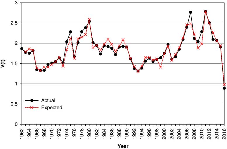
Figure 5 Actual and expected values of Cover, V(t), 1963–2016.

8.7 The response of Cover to changes in Earnings is large, almost one for one, in the current year, and smaller but negative in the following year. This can be explained plausibly. When Earnings increase, Cover also does so automatically unless Dividends are also changed. But companies may defer increases in Dividends till the following year, and if they occur then so Cover is reduced.

8.8 We discuss other aspects of the model for Cover in section 12 et seqq.

9. P/E Ratio

9.1 Once we have models for Cover and for Dividend Yield, we can calculate in any simulation the corresponding P/E ratio, but we can instead derive an explicit model for it. We denote it as M(t) (Multiple). The P/E Ratio, M(t)=P(t)/E(t)=P(t)/D(t)×D(t)/E(t), where E(t) is the Share Earnings Index and P(t) the Share Price Index. Thus

$$M\left( t \right)\, {\equals}\, {1 \mathord{\left/ {\vphantom {1 {\left( {V\left( t \right){\rm }{\times}Y\left( t \right)} \right)}}} \right. \kern-\nulldelimiterspace} {\left( {V\left( t \right){\rm }{\times}Y\left( t \right)} \right)}}$$

and

$$ML\left( t \right)\, {\equals}\, {\rm Ln}\left( {M\left( t \right)} \right)\, {\equals}\, -\left( {VL\left( t \right){\plus}YL\left( t \right)} \right)$$

9.2 Using the formulae for Cover and Yield we get:

$$\eqalignno{ \qquad ML\left( t \right)\, {\equals}\, & -\left( {VL\left( t \right){\plus}YL\left( t \right)} \right) \cr \, {\equals}\, & {\minus}\left\{ {VMUL{\plus}VW.I\left( t \right){\plus}VA.VN\left( {t-1} \right){\plus}VE1.EE\left( t \right){\plus}VE2.EE\left( {t-1} \right)} \right. \cr & \left. { {\plus}VY1.YE\left( t \right){\plus}VY2.YE\left( {t-1} \right){\plus}VSD.VZ\left( t \right)} \right\} \cr &-{\rm }\left\{ {YMUL{\plus}YW.I\left( t \right){\plus}YA.YN\left( {t-1} \right){\plus}YSD.YZ\left( t \right)} \right\} \cr \, {\equals}\, & -\{ {( {VMUL{\plus}YMUL} ){\plus}( {VW{\plus}YW} ).I( t ){\plus}VA.VN( {t-1} ){\plus}YA.YN( {t-1} )} \cr & \quad {\plus}VE1.EE\left( t \right){\plus}VE2.EE\left( {t-1} \right){\plus}VY1.YE\left( t \right){\plus}VY2.YE\left( {t-1} \right) \cr &\left. { \quad {\plus}VSD.VZ\left( t \right){\plus}YSD.YZ\left( t \right)} \right\} $$

9.3 This suggests that a plausible direct model for Multiple, omitting all reference to Dividend Yield and to Cover, might be

$$\eqalignno{ & MN\left( t \right)\, {\equals}\, MA.MN\left( {t-1} \right){\plus}ME1.EE\left( {\rm t} \right){\plus}ME2.EE\left( {t-1} \right){\plus}MSD.MZ\left( t \right) \cr & ML\left( t \right)\, {\equals}\, MMUL{\plus}MW.I\left( t \right){\plus}MN\left( t \right) $$

9.4 We fit this formula, in a series of steps, and we show the results in Table 6. The improvement in Step 4, including ME2, is small, and the value of the coefficient is only marginally significant, but we leave it in for comparison. We see that the estimate for MW is −2.9445, and we can calculate

$$-(VW{\plus}YW)\, {\equals}\, -\left( {1.6921{\plus}1.4986} \right)\, {\equals}\, -3.1907$$

We then see that VA=0.9266, YA=0.6945, and MA=0.7141, in between the first two, though closer to YA. The value of ME1 is −1.0017 compared with VE1=0.9049, and ME2=0.4182 compared with VE2=−0.2832, so they are not too far apart, allowing for the change in sign. Next we calculate MMUL=Ln(MMU)=Ln(16.4678)=2.8014 and also

$$-{\rm }\left( {VMUL{\plus}YMUL} \right)\, {\equals}\, -\left( {{\rm Ln}\left( {1.4794} \right){\plus}{\rm Ln}\left( {0.0383} \right)} \right)\, {\equals}\, 2.9232$$

Finally we see that MSD=0.1592 and √(VSD ²+YSD ²)=√(0.0538²+0.1667²)=0.1752. The formulae are therefore seen to be reasonably equivalent. However, the direct forecasting of ML seems a little better than the two-stage one, in that the standard deviation is lower, although with Y and V there is more information.

Table 6 Results for Price/Earnings Ratio.

9.5 We show in Figure 6 the actual values of M(t) at annual intervals, along with two estimates, one from the direct model, the second from V and Y. In both cases we show the exponential of the expected value. These are quite close in almost every year. However, the models are not conditional only on ℱ _t , but also on other information at the end of year t, and they are not based on the same information.

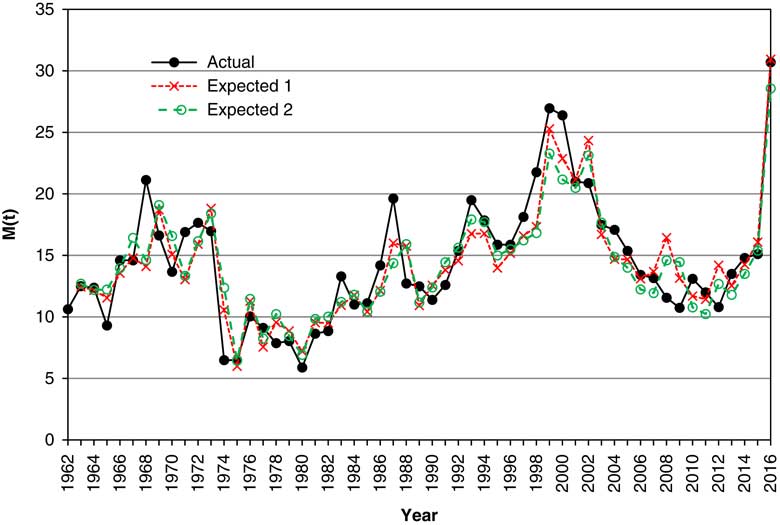
Figure 6 Actual and expected values of Price/Earnings ratio, M(t), 1963–2016, with the expected calculated in two different ways.

9.6 We compare the two approaches further when we consider forecasting in section 13.

10. Share Dividends and Prices

10.1 Given values for Earnings and Cover, we can calculate Share Dividends, and given values for Dividends and Dividend Yields, we can calculate Share Prices. Calculating simulated values is easy, but getting formulae for the variances and covariances of forecast values is more tedious, though possible. However, if we wish to compare results from the new models with those from the old, we need to use the old model for Share Dividends, and it would be better to have this updated to 2016.

10.2 The old model for dividends is

$$\eqalignno{ & DM\left( t \right)\, {\equals}\, DD.I\left( t \right){\plus}(1{\minus}DD).DM(t{\minus}1) \cr & DI\left( t \right)\, {\equals}\, DW.DM\left( t \right){\plus}DX.I\left( t \right) \cr & K\left( t \right)\, {\equals}\, DI\left( t \right){\plus}DMU{\plus}DY.YE(t{\minus}1){\plus}DB.DE(t{\minus}1){\plus}DE\left( t \right) \cr & DL\left( t \right)\, {\equals}\, DL(t{\minus}1){\plus}K\left( t \right) \cr & D\left( t \right)\, {\equals}\, {\rm exp}\left( {DL\left( t \right)} \right) $$

10.3 As with Dividend Yields, we have three series for Dividends, the original from 1923 onwards, based on Adjusted Dividend Yields, the Unadjusted equivalent and the Composite series, from 1963 onwards. In the left-hand column of Table 7, we show the estimated values of the parameters for the Unadjusted series from 1923 to 2016. The parameter values are not very different from those for the Adjusted series found in 2009 and shown in Part 1.

Table 7 Results for Share Dividends.

10.4 We fit the old model to the Composite Dividend Index data for the period since 1963 and show the results in the rightmost column of Table 7. If we include the DB term the value of DW becomes negative, which is not realistic, so we omit the DB term. Apart from this term, the values of the parameters are reasonably similar to those for the longer period.

10.5 For comparison with the new model, we choose the result for the Unadjusted series for Dividend Yield and Share Dividends, using the data from 1923. Others might prefer a different comparator. However, the long-term mean rate of growth of dividends, which we can call DMU*, is calculated with its individual model as

$$DMU^{\asterisk}\, {\equals}\, DMU{\plus}(DW{\plus}DX){\times}QMU\, {\equals}\, DMU{\plus}QMU$$

since DW+DX is always taken as equal to 1. The value of this then depends on which value of QMU we take. At the foot of Table 8 we show the values of QMU for the corresponding periods, from Table 2, and the corresponding values of DMU*. There is a considerable difference in the values of DMU* between the periods starting in 1923 and that starting in 1963. The values of DMU* can be compared with those for EMU* given in Table 7, since both represent the long-term rate of (nominal) growth in Earnings, Dividends and Share Prices, an important aspect of any simulation model.

Table 8 Suggested input sets, working sets and output sets of variables.

11. The Model So Far

11.1 At this point it is convenient to summarise the model so far. We do not, in this paper, discuss wages or interest rates, although they are parts of the complete model. We state the models we shall generally use in the examples in the rest of this paper, giving the parameter values that we shall use. We round each parameter value to four decimal places, and use the rounded values hereafter.

11.2 However, when we wish to make comparisons between different models, and in order to be more in possible accordance with current conditions, we adjust certain mean values. The fitted value of QMU, the mean rate of increase of Retail Prices from 1923 to 2016, is 0.0424. This seems high, in view of the much lower rate of increase of recent years so, we set QMU=0.025. The rate of growth of Share Earnings in excess of Retail Prices is given by EMU and the fitted value of this up to 2016 is −0.0041. However, up to 2015 the value was 0.0099. The low value is caused entirely by the massive drop in Earnings in the last year, but it seems more plausible to use the earlier figure for the future, so we set EMU=0.01. In order to make comparisons with our original model we need the mean rate of growth of Dividends in excess of Retail Prices in that model, DMU, to equal EMU. So we also set DMU to equal 0.01, which is not too different from the fitted value, also over the period 1923–2016, of 0.0111. The neutral initial conditions need to be calculated relative to these adjusted values.

11.3 Retail Prices, Q(t): for these we use the values fitted over the period 1923–2016:

$$QA\, {\equals}\, 0.5718;\,QMU\, {\equals}\, 0.0424\,\left( {{\rm fitted}} \right)\,{\rm or}\,0.025\,\left( {{\rm adjusted}} \right);\,QSD\, {\equals}\, 0.0385$$

11.4 Dividend yield, Y(t): for these we use the values for the Unadjusted index fitted over the period 1923–2016; these use the published Actual Yield, so there is no need for any further adjustment:

$$YW\, {\equals}\, 1.4225;\,YA\, {\equals}\, 0.6518;\,YMU\, {\equals}\, 0.0363\,\left( {3.63\,\%\,} \right);\,YSD\, {\equals}\, 0.1588$$

11.5 Earnings, E(t): for these we use the values for the Composite index fitted over the period 1963–2016, with a restriction that EQ1+EQ2=1:

$$\eqalignno{ & EQ1\, {\equals}\, 2.8494;\,EQ2\, {\equals}\, 1{\minus}EQ1\, {\equals}\, -1.8494;\,EY\, {\equals}\, -0.3887 \cr & EMU\, {\equals}\, -0.0041\,\left( {{\rm fitted}} \right)\,{\rm or}\,0.01\,\left( {{\rm adjusted}} \right);\,ESD\, {\equals}\, 0.1516 $$

11.6 Cover, V(t): for these we use the parameter values fitted for the Composite index over the period 1963–2016:

$$\eqalignno{ & VA\, {\equals}\, 0.9266;\,VE1\, {\equals}\, 0.9049;\,VE2\, {\equals}\, -0.2832;\,VY1\, {\equals}\, -0.1511;\,VY2\, {\equals}\, -0.1866 \cr & VW\, {\equals}\, 1.6921;\,VMU\, {\equals}\, 1.4794;\,VSD\, {\equals}\, 0.0538 $$

11.7 We can make comparisons for the P/E Ratio and the Dividend series derived in two different ways, either from the other series modelled, or from the directly modelled series, as noted below.

11.8 P/E ratios, M(t): for these we use the Composite index fitted over the period 1963–2016:

$$\eqalignno{ & MA\, {\equals}\, 0.7141;\,ME1\, {\equals}\, -1.0017;\,ME2\, {\equals}\, 0.4182;\,MW\, {\equals}\, -2.9445 \cr & MMU\, {\equals}\, 16.4678;\,MSD\, {\equals}\, 0.1592 $$

11.9 Dividends, D(t): for these we use the Unadjusted index fitted over the period 1923–2016:

$$\eqalignno{ & DW\, {\equals}\, 0.4232;\,DD\, {\equals}\, 0.1628;\,DX\, {\equals}\, 1{\minus}DW\, {\equals}\, 0.5768;\,DY\, {\equals}\, -0.1995 \cr & DB\, {\equals}\, 0.4827;\,DMU\, {\equals}\, 0.0111\,\left( {{\rm fitted}} \right)\,{\rm or}\,0.01\,\left( {{\rm adjusted}} \right);\,DSD\, {\equals}\, 0.0720 $$

11.10 We use initial conditions as at June 2016 (t=0), which are

$$\eqalignno{ & Q\left( 0 \right)\, {\equals}\, 263.1;\,I\left( 0 \right)\, {\equals}\, 0.0161;\,I\left( {-1} \right)\, {\equals}\, 0.0101 \cr & Y\left( 0 \right)\, {\equals}\, 3.66\,\%\,;\,Y\left( 0 \right)\, {\equals}\, 3.46\,\%\, \cr & E\left( 0 \right)\, {\equals}\, 114.51;\,EE\left( 0 \right)\, {\equals}\, -0.7352 \cr & V\left( 0 \right)\, {\equals}\, 0.8900;\,DM\left( 0 \right)\, {\equals}\, 0.0257;\,DE\left( 0 \right)\, {\equals}\, 0.0019 $$

11.11 Additional initial conditions that may be required are M(0), which can be calculated as 1/(V(0×Y(0))=30.70, and D(0), which can be calculated as E(0)/V(0=128.67. This is the same value as we get from the 1923–2016 data, since we arranged the values to run into the same series for the more recent years.

11.12 We also, for comparison, use initial values as at June 2015, which are

$$\eqalignno{ & Q\left( 0 \right)\, {\equals}\, 258.9;\,I\left( 0 \right)\, {\equals}\, 0.0101;\,I\left( {-1} \right)\, {\equals}\, 0.0261 \cr & Y\left( 0 \right)\, {\equals}\, 3.46\,\%\,;\,Y\left( {-1} \right)\, {\equals}\, 3.27\,\%\, \cr & E\left( 0 \right)\, {\equals}\, 236.31;\,EE\left( 0 \right)\, {\equals}\, -0.0432 \cr & V\left( 0 \right)\, {\equals}\, 1.9128;\,DM\left( 0 \right)\, {\equals}\, 0.0276;\,DE\left( 0 \right)\, {\equals}\, 0.0279 $$

12. State Variables, Initial Conditions and Long-Term Means and Variances

12.1 In Part 2 of this series, we discussed what variables were required in sets of variables for inputs, for working and for output. The new models are straightforward in this respect. In Table 8 we show our suggested sets of variables for the relevant cases.

12.2 Since the Earnings model depends only on the most recent values of I(t), unlike the original model for Dividends which depended on an exponentially weighted moving average of all past values, DM(t), the inputs required for Earnings are simpler. However, we still use EE(t−1), so the input set must contain EE(0). We include EE(t) in the output set, since one might wish to continue a simulation at its ending point. To help potential users of the model we show certain of these values in Table 9, based on the new parameter values as given in section 11. Observe how the values of E(0) and EE(0) reduce sharply from February 2016.

Table 9 Initial conditions for the Retail Prices, Dividend Yield, Earnings Index and Cover models in 2015 and part of 2016.

12.3 In Part 2 we also suggested that there might be occasions when one wished to use “neutral initial conditions” rather than market conditions at any particular date. For the relevant series and with the new parameters, including the adjusted means, these are

$$\eqalignno{ & I\left( 0 \right)\, {\equals}\, I\left( {-1} \right)\, {\equals}\, QMU\, {\equals}\, 0.025 \cr & Y\left( 0 \right)\, {\equals}\, YMU.{\rm exp}\left( {YW.QMU} \right)\, {\equals}\, 3.83\,\%\,{\times}{\rm exp}\left( {1.3665{\times}0.025} \right)\, {\equals}\, 3.9631\,\%\, \cr & YE\left( 0 \right)\, {\equals}\, EE\left( 0 \right)\, {\equals}\, 0 \cr & V\left( 0 \right)\, {\equals}\, VMU.{\rm exp}\left( {VW.QMU} \right)\, {\equals}\, 1.4373{\times}{\rm exp}\left( {1.5350{\times}0.0025} \right)\, {\equals}\, 1.4935 $$

12.4 In Part 2 we suggested that an alternative way of starting a simulation would be to use random values for the initial conditions, chosen from their long-term distribution. To do this we need the long-term values. In the Appendix of Part 2, we quoted formulae for the means and variances of the projected values of the variables at future time t, conditional on conditions at time t=0. As t→∞ we get the long-term values. In the Appendix of this paper, we give formula for the means and variances for those among the new variables that are linear (so excluding exponentiated ones), that is: L, EL, VL, ML, DL, and PL, the last three each calculated in two different ways. We denote by ML the value calculated from YL and VL, and by ML2 the value calculated directly. By DL and PL we denote the values calculated with the new model, based on EL; and by DL2 and PL2 we denote the values calculated from the old model for DL, but with updated parameters.

12.5 The long-term correlation coefficients can also be calculated by formulae, but these are extremely tedious (as can be seen from Part 2). Instead we estimate these by simulation, using one million simulations for 500 years each, and taking as estimated correlation coefficients the average of those calculated for years 491–500.

12.6 The statistics of the relevant variables, assuming the adjusted values of QMU, EMU, and DMU, are shown in Table 10. We omit those variables whose long-term mean or variance is infinite.

Table 10 Long-term means, standard deviation and correlation coefficients of selected variables.

13. Forecasts

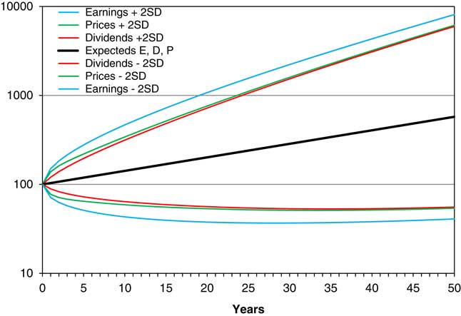
13.1 Using the forecast means and standard deviations described in section 12, we show in Figure 7 the means and means ± 2 standard deviations, for E, D, and P, all assuming the new parameters, with adjusted values for the means, and assuming neutral initial parameters. Strictly what we show is exp(E[EL]), etc., that is the exponent of the mean of EL. This is not the expected value of E, because, assuming normally distributed residuals for L, then E is lognormally distributed with mean exp(E[EL]+Var[EL]/2). One can think of them as “central forecasts”, without being precise about whether this is mean, median, or another value near the centre. We start E, D, and P all at the same value, of 100. Each grows at a continuous compound rate of 0.035 per year, so the lines for the mean values are, on a logarithmic scale, the same straight line.

Figure 7 Means and means ±2 s.d., of E, D and P assuming neutral initial conditions, forecast for 50 years.

13.2 Note that the “expanding funnel of doubt” for Earnings is wider than those for Dividend and Prices, which in the long run are quite similar, though initially Prices have a wider spread than Dividends. Although the spread of all three is wide, the values are quite closely correlated, so in any one simulation the three would move closer together.

13.3 We can calculate the same for YL, VL, and ML, but we do not show the diagram. All three have means which remain constant at the neutral initial conditions, and the expanding funnel after about 5 years approaches the long-term constant ranges, which for Y are about 2.4%–5.8%, for V are about 0.8–3.0 and for M are about 8–36. Assuming normality of the residuals, these ranges contain about 95% of the distribution, but there is a reasonable chance of future values lying outside these ranges, as indeed past values have done.

13.4 We can calculate the same statistics for D and P, using the old model, but with updated parameters, and we compare these with those for the new model in Figure 8.

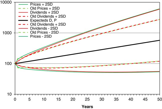
Figure 8 Means and means ±2 s.d., of D and P, assuming neutral initial conditions, for new and old models, forecast for 50 years.

13.5 We see that the funnel of doubt for the new model is quite a bit wider than for the old, though the lines for Dividends and Prices are very close in both. We assume that this is primarily because of the large uncertainty about future earnings, observed in the value of ESD, which we see from Table 4 went up from 0.1141 when we estimated it in 2015 to 0.1516 when we estimated it again 2016. If we use the 2015 parameters, the old and new results are very similar. One extreme year can make a big difference; since at this stage we are assuming normally distributed residuals, this extreme value affects the standard deviation; were we to assume a different distribution for residuals, the results would probably be different.

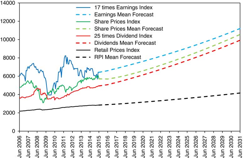
13.6 We can do the same calculations starting with initial conditions as at any chosen date. We start by taking initial conditions as at June 2015, though with the parameters as fitted up to 2016. In Figure 9 we show the actual values, monthly, for 9 years from June 2006 to June 2015 for RPI, Share Prices (scaled), 17 times Earnings and 25 times Dividends (the same values as in Figure 1), together with mean (or central) forecasts of these variables for the next 16 years.

Figure 9 RPI, Share Price Index, 25 times Dividends and 17 times Earnings, actual June 2006 to June 2015 monthly and mean forecasts June 2015 to June 2031 yearly, with initial conditions as at June 2015.

13.7 One can see that the mean forecasts are tidily well behaved, with Earnings and Dividends increasing at about 3.5% a year, and Share Prices following after a short dip. This is because the June 2015 conditions were not very far from neutral.

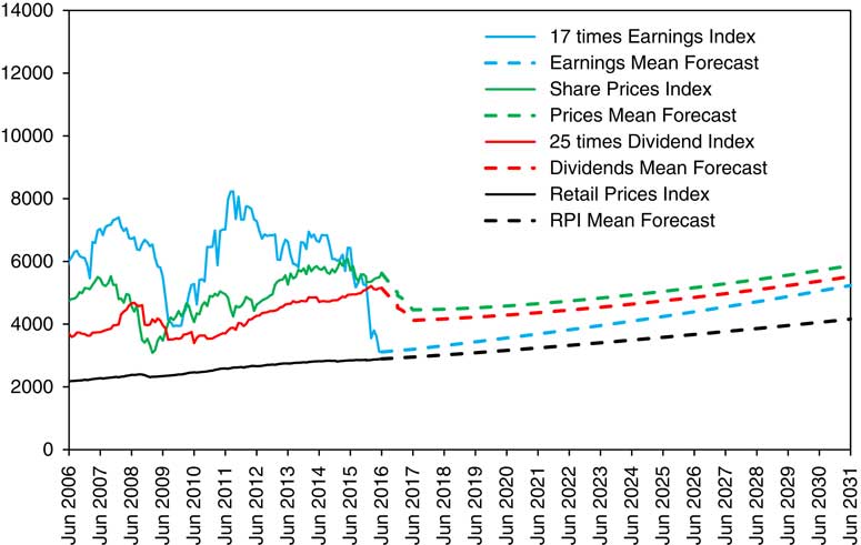
13.8 In Figure 10 we show the same, but with initial conditions as at June 2016, and with actual up to 2016 and forecasts thereafter. It is on the same vertical scale as Figure 9, and one can see how much lower the longer-term forecasts are. We see the mean forecast value of the RPI increasing at a steady 0.025 continuously compounded per year, almost the same as in 2015. Earnings, according to the model, are rising at a rate of about 0.035 per year. The forecasts for Dividends and Share Prices show a drop of 20% in the first year and a rather slow rise thereafter of 1%–2% a year, with a longer-term level only a little over half that of the 2015 forecast. The mean forecast for Dividends reaches the 2016 level again by 2029 and that for Share Prices by 2030. In any actual simulation the possible results would be much wider than these “forecasts” suggest, and in the real world the uncertainty is at least as great. With random simulation any result is possible, even if there is a low probability, so we not be surprised to see substantial falls in Dividends and Share Prices in the next year or two, but we not be surprised at any other possible result. On the other hand, our model has ruled it out as impossible that Earnings for the whole Index could turn negative, though in the real world it might not be impossible.

Figure 10 RPI, Share Price Index, 25 times Dividends and 17 times Earnings, actual June 2006 to June 2016 monthly and mean forecasts June 2016 to June 2031 yearly, with initial conditions as at June 2016.

13.9 We are reminded of the situation in 1974, when one of us was actively involved in economic and investment research. It was a year of great political and economic uncertainty. By September 1974, share prices had dropped to about one-third of their previous peak in August 1972, and the gross dividend yield on the ASI was over 10%. He remembers writing that one might expect the yield in a year’s time to be closer to the more normal 5%, but whether this would be because dividends would halve or prices would double was quite uncertain, because of the political policy. Although share prices sank further by the end of 1974, they nearly doubled in the first 2 months of 1975, rose further in the rest of the year and by September 1975 the dividend yield was just below 6%. During this whole period dividends rose fairly steadily and earnings (on the “500” NFI), rose quite strongly (see Figure 1).

13.10 The position this time is reversed, with Earnings falling heavily, halving over the year 2015–2016, but Dividends and Prices continuing as before, and there is almost no public comment on this. Would we not expect either Dividends and Prices to halve, or Earnings to double? Our model expects Dividends and Prices to almost halve as compared with what they might have been on the basis of the 2015 forecasts, though slipping slowly rather than suddenly. So, if dividends in the next few years are expected to be at half the level expected in June 2015, why have share prices not already halved too?

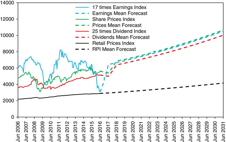
13.11 The reply may be that those in “the market” fully expect Earnings to recover sharply, so justifying the present prices. We can reflect this in the model by using a technique described in section 8 of Part 2, where it is described as using a “Select Period”. As at June 2016, we set the mean value of EE(2017) at 0.6976, rather than the usual 0, chosen so that the expected value of EL(2017), as forecast in 2016, is the same as the actual value of EL(2015).

13.12 We show the resulting mean forecasts in Figure 11. We see that Earnings, Dividends, and Prices follow a similar track to that forecast in 2015, after a fairly small fall in the latter two by June 2017. Forecast Earnings in 2031 are about 7% less, and forecast Dividends and Prices about 1% more than those forecast in 2015. But both any simulated futures and the real world have to have a large stochastic element wrapped around these central forecasts, and the real-world experience (of which there will be only one example) will almost certainly not follow any of these forecast patterns at all closely.

Figure 11 RPI, Share Price Index, 25 times Dividends and 17 times Earnings, actual June 2006 to June 2016 monthly and mean forecasts June 2016 to June 2031 yearly, with initial conditions as at June 2016, but with adjustment to EE(2017).

13.13 Such a large reversal of Earnings in 2017 raises another question. There is no evidence in our data so far of significant negative autocorrelation between the residuals of the earnings series in successive years, and such a large reversal would imply one. But it is possible to imagine a series which is generally random, with no autocorrelation, and is generally normally distributed, as the earnings residuals appeared to be up to 2015 (see Table 4), but if a very large random deviation occurred, which was well outside what one would expect with a normally distributed series, a large reversal might occur in the following year. Such a series might be not normally distributed, and might not have a normal “copula” connecting successive values; but this takes us outside the scope of our present investigation.

13.14 At the time of writing, April 2017, there is only a small sign of such a strong reversal. Between the end of June 2016 and the end of March 2017 Share Earnings rose by 23.2%, an amount well above average, but nothing like enough to compensate for the fall a year previously. Over the same period Share Prices rose by 13.5% and Dividends by 7.6%, so cover improved to 1.02 and the P/E ratio fell to 28.29. Those large companies with large losses in 2015 have not shown a strong reversal, but the market still seems content. Our model suggests that this will not last, but it is also possible that a “new normal” will be achieved, in which companies (overall, not each individually) adopt a policy of very small retentions, not attempting to finance expansion, and pay almost all of the available earnings out in dividend. This would be in line with a situation of no overall economic growth in the United Kingdom and other developed countries, and a static environment. In the course of human history, the usual position has been one of economic stability, and the great economic growth of the last 200 years and more has been exceptional. At some point it may have gone as far as it can and may not continue. But this is a topic well beyond the scope of this paper.

14. Neutralising Parameters

14.1 In section 7 of Part 2, we described how one might choose what we called “neutralising parameters”, that is, values of the parameters, in particular the means of the series, so that the market conditions at any data are the neutral initial condition for those parameters. We showed that this was possible, though not quite straightforward for the variables in the model at that time.

14.2 With the new model, some items remain as before, such as Y(t). Then, since the long-term mean rate of growth of dividend is the same as that of earnings, the rationale that we applied to DMU previously can be applied in effectively the same way to EMU.

14.3 Cover, however, is a problem. V(t) is similar to Y(t), and normally one could use the same method, taking the current value of V(t) and making an adjustment for the effect of I(t) through the VW term. This would have worked until the end of 2015. But when Cover drops below 1.0, one cannot take such a value as a possible long-term mean. In the long run, Dividends cannot persistently exceed Earnings, for any one company or for the market as a whole. Cover is not determined by the market, but by the directors or shareholders of companies, so it may not be helpful to think of a market-neutral value of it. We have suggested in section 13 an exceptional adjustment to next year’s Earnings through a special mean value for EE(2017). This would be consistent with a forecast value of V(2017) of around 2.27, which is above average; but this pays no attention to a possible abnormal change in Dividends. We conclude that one who wishes to choose values for neutralising parameters for the new variables in the model has to use their own judgement. There is no simple way to model it.

15. Stochastic Interpolation

15.1 In Parts 3A, 3B, and 3C we described how one could model stochastic interpolation for the various series, assuming that values had been simulated for an annual model and one wished to add values for intervening months thorough each year. We have made the same investigations for the new series, Earnings, EL(t), and Cover, V(t), considering Brownian bridges for both, and also Ornstein–Uhlenbeck bridges for the latter. We do not show all our calculations, but our conclusions are that Brownian bridges suit both series, but with modifications as in Parts 3B and 3C.

15.2 For earnings we suggest a Brownian bridge, with a varying monthly standard deviation, σ(t), whose square varies with the square of the deviation of the change in EL during the year, ELD(t)=EL(t+1)−EL(t)=L(t), from its mean value, ESC:

$$\sigma \left( t \right)^{2} \, {\equals}\, ESM\left( t \right)^{2} \, {\equals}\, ESA{\plus}ESB.(ELD\left( t \right){\minus}ESC)^{2} $$

where ESA=0.000671, ESB=0.024548, and ESC=0.049681. There are no additional correlations, except with Cover, which is introduced below. The forwards and sideways deviations have very large kurtosis in many months, and even when they are standardised the forwards deviations for some months have large kurtosis.

15.3 For Cover we also suggest a Brownian bridge with a monthly standard deviation whose square varies with the square of the change in VL during the year, so that VLD(t)=VL(t+1)−VL(t):

$$\sigma \left( t \right)^{2} \, {\equals}\, VSM\left( t \right)^{2} \, {\equals}\, VSA{\plus}VSB.VLD\left( t \right)^{2} $$

where VSA=0.008270 and VSB=0.028582. We find no evidence for correlation of the standardised forwards deviations in the same month from one year to the next, but there is a very strong correlation with the standardised residual of Earnings in the same month, of 0.9321, which needs to be included. As for Earnings the forwards and sideways deviations have very large kurtosis in many months, both unstandardised and standardised, but these are connected also with the deviations for Earnings.

16. Examples

16.1 We are now able to carry out simulations, first deriving annual values of the relevant variables, then filling in values at monthly intervals. We carried out 100 independent simulations, each for 30 years, all based on the initial conditions as at June 2016, without the “select period” adjustment described in section 13, and with the value of QMU assumed to be 0.025. We then select the values of the accumulating variables (Q, E, D, and P) at the end of the 30-year period, and also of the ratio variables (Y, V and M). We chose to display the simulations that give the third highest value and the third lowest value of E at that time, calling them “High simulation” and “Low simulation”. In Table 11 we show the maximum and minimum values of the selected variables, and the values in the High and Low simulations.

Table 11 Values of selected variables in selected simulations out of 20, at duration 30 years.

16.2 For the accumulation variables the values at duration 30 are often either the highest attained or close to that, but they may not be. The values of the ratio variables have no reason to be very high or very low at that time. In Table 12, we show (as percentages) the probability of these values, assuming a cumulative normal distribution function, taking account of the means and standard deviations calculated as in section 12. We see that the values of the accumulation variables in the High simulation are mostly exceptionally high, and in fact the values of Q and D in this simulation are the maxima. Those in the Low simulation are not exceptionally low. The ratio variables are much more evenly balanced.

Table 12 Probability, assuming normality, of values of variables shown in Table 10.

16.3 Picking the third highest and third lowest values is roughly equivalent to a 2.5% probability at each tail, so there is a sort of 95% chance that the actual future (if it follows the model) will lie somewhere between these. But the results are very far apart. This indicates how the model draws attention to the uncertainty about forecasting these investment variables. And we have assumed normally distributed innovations, whereas the residuals from the past data are generally more fat tailed, and we have made no allowance for parameter uncertainty. We hope to look at both of these points in later parts of this series.

16.4 In Figure 12 we show values for the High simulation of Q, 17E, 25D and P, all scaled to fit the logarithmic scale conveniently, with past data up to June 2016 in strong colours and simulated forecast data in paler colours. In Figure 13 we show the same for the Low simulation. We can see that the High simulation shows very good returns, the Low very poor ones. Note that the vertical logarithmic scale is shown over different cycles for the two graphs.

Figure 12 Values of Retail Price Index (Q), Share Price Index (P), 25 times Dividend Index (D) and 17 times Earnings Index (E), all scaled, with actual data from January 1996 to June 2016 and high simulation values from June 2016 to June 2046.

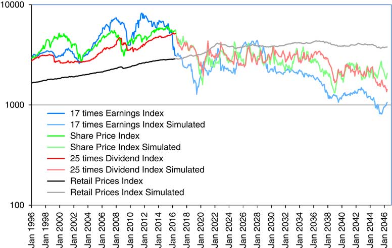
Figure 13 Values of Retail Price Index (Q), Share Price Index (P), 25 times Dividend Index (D) and 17 times Earnings Index (E), all scaled, with actual data from January 1996 to June 2016 and low simulation values from June 2016 to June 2046.

16.5 In Figures 14 and 15 we show, for the High simulation and Low simulation, the values of dividend yield (Y), P/E ratio (M), and cover (V) multiplied by 10, for the same periods, with actual data to June 2016 again in strong colours, and simulated values in paler colours. Note that Cover falls below 1.0 occasionally for the High simulation, and quite often in the Low simulation.

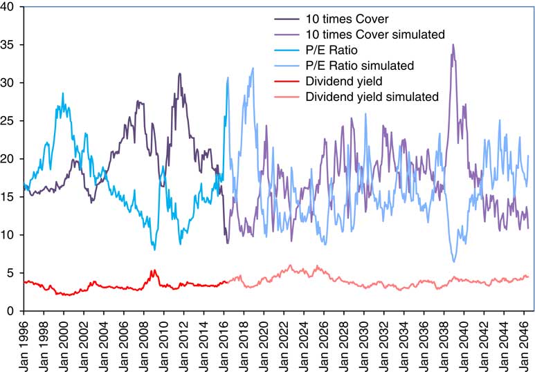
Figure 14 Values of Dividend Yield (Y), Price/Earnings (P/E) Ratio (M) and 10 times Cover (V), with actual data from January 1996 to June 2016 and high simulation values from June 2016 to June 2046.

Figure 15 Values of Dividend Yield (Y), Price/Earnings (P/E) Ratio (M) and 10 times Cover (V), with actual data from January 1996 to June 2016 and low simulation values from June 2016 to June 2046.

16.6 It appears to us that the general behaviour of all the series on both sides of the division between past actual and future simulated at June 2016 is rather similar. This may be in the eye of the beholder, but the overall pattern is not conspicuously different. This suggests that the simulation models that we suggest are not unreasonable.