


Introduction
Silverleaf nightshade (Solanum elaeagnifolium Cav., Solanaceae) is considered one of the most invasive weeds worldwide. It is mainly found in arid and semiarid bioclimatic regions with temperate to warm winters (Balah and Abdel Razek Reference Balah and AbdelRazek2020). Solanum elaeagnifolium is indigenous to the western United States and northern Mexico, but has spread to other parts of the world, including Australia, Greece, Morocco, and parts of southern Europe and the Mediterranean region (Brunel Reference Brunel2011; Mekki Reference Mekki2007; Stanton et al. Reference Stanton, Heap, Carter, Wu and Panetta2009; Uludag et al. Reference Uludag, Gbehounou, Kashefi, Bouhache, Bon, Bell and Lagopodi2016; Zernov and Mirzayeva Reference Zernov and Mirzayeva2016). It is a perennial weed that reproduces both sexually, through seed production, and asexually, through vegetative growth of rhizomes (Hardin et al. Reference Hardin, Doerksen, Herndon and Hobson1972; Knapp et al. Reference Knapp, Sagona, Carbonell and Chiarini2017). By virtue of these characteristics, S. elaeagnifolium is a highly noxious weed that can colonize and thrive in various ecological niches, such as natural reservations, riverbanks, and cultivated fields (Ilçim and Behçet Reference Ilçim and Behçet2007; Krigas et al. Reference Krigas, Tsiafouli, Katsoulis, Votsi and van Kleunen2021; Uludag et al. Reference Uludag, Gbehounou, Kashefi, Bouhache, Bon, Bell and Lagopodi2016). Solanum elaeagnifolium was introduced into Israel in the 1950s and since then has spread throughout the country, becoming a serious problem in fields of irrigated summer crops, such as cotton (Gossypium hirsutum L.), processing tomato (Solanum lycopersicum L.), and watermelon [Citrullus lanatus (Thunb.) Matsum. & Nikai], and often causing significant economic losses (Stanton et al. Reference Stanton, Heap, Carter, Wu and Panetta2009).
The control of S. elaeagnifolium is highly challenging due to its vigorous vegetative growth and extensive root system (Qasem et al. Reference Qasem, Al Abdallat and Hasan2019). Although glyphosate and ammonium sulfate can provide effective control (Gitsopoulos et al. Reference Gitsopoulos, Damalas and Georgoulas2017), the lack of selectivity of the two herbicides limits their usage for control scenarios such as preemergence and direct spraying. Other herbicides that have shown efficacy (e.g., imazapyr, aminopyralid, and picloram) are not suitable for agricultural purposes (Wu et al. Reference Wu, Stanton and Lemerle2016). Furthermore, mechanical control tools, such as tillage and cultivation, are not practicable for S. elaeagnifolium, because the use of mechanical machinery can break the root system and spread the propagules throughout the field (Gitsopoulos et al. Reference Gitsopoulos, Damalas and Georgoulas2017; Qasem et al. Reference Qasem, Al Abdallat and Hasan2019; Wu et al. Reference Wu, Stanton and Lemerle2016). These limitations create the need for novel ecologically based control approaches that can be integrated into the currently used control methods. However, the development of such methods will require extensive biological and ecological knowledge about the weed (Bajwa et al. Reference Bajwa, Mahajan and Chauhan2015).
Ecological control tools are based on data about key phases in a weed’s life cycle and phenology, such as the timing and magnitude of seed germination, which determine the establishment of the weed in the field (Forcella et al. Reference Forcella, Benech Arnold, Sanchez and Ghersa2000; Grundy et al. Reference Grundy, Peters, Rasmussen, Hartmann, Sattin, Andersson, Mead, Murdoch and Forcella2003; Rodriguez et al. Reference Rodriguez, Kruk and Satorre2020). Because S. elaeagnifolium typically produces up to 9,000 seeds per plant (Boyd and Murray Reference Boyd and Murray1982), effective control of young seedlings can make a significant contribution to the overall management of this weed. Seed germination is affected by various environmental conditions, with temperature being the most important of these under irrigated field conditions (Derakhshan et al. Reference Derakhshan, Gherekhloo, Vidal and De Prado2014; Garcia-Huidobro et al. Reference Garcia-Huidobro, Monteith and Squire1982; Guillemin et al. Reference Guillemin, Gardarin, Granger, Reibel, Munier-Jolain and Colbach2013; Shrestha et al., Reference Shrestha, Roman, Thomas, Swanton and Thomas1999). Nonetheless, studies investigating the impact of temperature on germination in S. elaeagnifolium are scarce. Among those that have been conducted, Boyd and Murray (Reference Boyd and Murray1982) evaluated the germination of S. elaeagnifolium under various environmental conditions. They found increased germination rates under an alternating temperature regime, with a maximal rate of 57% under a 20/30 C regime. Similar results were obtained by Balah et al. (Reference Balah, Hassany and Mousa2021), who showed optimal germination under an alternating temperature regime of 20/30 C, but at a lower rate of 33%. A slightly different germination pattern was revealed by Stanton et al. (Reference Stanton, Wu and Lemerle2012), with 15/25 C as the optimal temperature regime for germination. These studies provided descriptive data about the impact of temperature on S. elaeagnifolium germination, but they lacked information on cardinal temperatures that could facilitate smart decision making regarding the control of this weed, for example, temperature-based germination prediction models.
Temperature measurements establish the basis for a number of weed germination predictive models, many of which use an empirical approach (Cochavi et al. Reference Cochavi, Goldwasser, Horesh, Igbariya and Lati2018; Doyle Reference Doyle1991; Hosseini et al. Reference Hosseini, Ahmadvand, Oveisi, Morshedi and Gonzalez-Andujar2017). The concept of these empirical models is based on thermal time units, that is, summing heat units above minimal temperature thresholds to predict the germination dynamics (Trudgill et al. Reference Trudgill, Honek, Li and Van Straalen2005). The development of these predictive models is based on preliminary data about the temperature thresholds (i.e., cardinal temperatures) for weed germination, such as the base temperature (at or below which germination does not occur), the optimal temperature (which supports the maximal germination rate), and the ceiling temperature (at or beyond which germination is zero) (Goldwasser et al. Reference Goldwasser, Miryamchik, Rubin and Eizenberg2016; Hardegree Reference Hardegree2006; Mesgaran et al. Reference Mesgaran, Onofri, Mashhadi and Cousens2017). However, no previous study has determined cardinal temperatures for S. elaeagnifolium, and hence there are no predictive models for S. elaeagnifolium seed germination. In addition, germination patterns in different S. elaeagnifolium populations have not been examined, and more information is needed at the local level about the variation of cardinal temperatures for S. elaeagnifolium populations in different climate zones in Israel.
The main objective of this study was to determine the effect of temperature on seed germination in three specific S. elaeagnifolium populations growing in different environments in Israel. To this end, the specific objectives of the study were: (1) to estimate the germination proportion and dynamics of S. elaeagnifolium under constant temperatures and under different alternating temperature regimes; (2) to determine the cardinal germination temperatures for three specific populations of S. elaeagnifolium; and (3) to develop a prediction model for S. elaeagnifolium germination dynamics and compare the germination patterns and cardinal temperatures for the three populations growing under different environmental conditions.
Material and Methods
Plant Material
Berries were collected from three populations of S. elaeagnifolium growing in fields located at Kibbutz Kfar Blum in the Hula Valley (33.16°N, 35.59°E), at the Newe Ya’ar Research Center in the Jezreel Valley (32.70°N, 35.18°E), and at Kibbutz Urim (31.30°N, 34.52°E) in the Negev Desert. The berries were removed from the plants and crushed, and the seeds were washed out and collected on a sieve under running water. The seeds were air-dried in a net house for 2 wk and stored at 4 C until use.
Experimental Setup
All experiments were conducted in the laboratory at the Newe Ya’ar Research Center from July to September 2019. Seed germination was evaluated by placing batches of 25 S. elaeagnifolium seeds in 90-mm-diameter petri dishes on filter paper (Whatman No. 1, Whatman, Maidstone, UK) presoaked for 24 h in deionized water. The photoperiod was maintained at 12 h:12 h (light:full darkness), according to Stanton et al. (Reference Stanton, Wu and Lemerle2012). Germinated seeds in each petri dish were counted each day at 11:00 AM. and then removed, until no additional germinations were observed over a period of 4 d. Seeds were considered to be germinated when the observed radicle was longer than 1 mm. All experiments were performed for all three populations. Experiments were arranged in a complete randomized design with four replications of treatments for both experiments. The experiments were repeated once. There was no experiment by treatment interaction; therefore, the data from both experiments were pulled and presented as eight replications of each treatment. All statistical analyses were performed using the R statistical environment (R Core Team 2020) together with the following packages: drc (Ritz et al. Reference Ritz, Baty, Streibig and Gerhard2015) and drcSeedGerm (Onofri et al. Reference Onofri, Benincasa, Mesgaran and Ritz2018).
Impact of an Alternating Temperature Regime on Germination
For this experiment, different alternating (12 h/12 h) temperature regimes based on two optimal average germination temperatures, 20 and 25 C, were tested (Balah et al. Reference Balah, Hassany and Mousa2021; Stanton et al. Reference Stanton, Wu and Lemerle2012). For each of these optimal temperatures, temperature regimes were set such that the difference between the day and night temperatures was 0, 2, 4, 6, 8, or 10 C, resulting in the following 12 regimes: 20/20, 19/21, 18/22, 17/23, 16/24, 15/25 C and 25/25, 24/26, 23/27, 22/28, 21/29, 20/30 C. The petri dishes containing the seeds were placed inside a growth chamber under these 12 alternating temperature regimes. In total, 144 petri dishes were examined (3 populations × 4 replicates × 6 temperature regimes × 2 optimal temperatures).
The data collected for each petri dish and temperature regime were used to parameterize a time-to-event model (Jensen et al. Reference Jensen, Wolkis, Keshtkar, Streibig and Ritz2020). For each S. elaeagnifolium population, the relationship between the cumulative seed germination and time (in days) under the 12 alternating temperature regimes were analyzed using a log-logistic equation:
 $$Y(t) = d/(1 + \exp \{ b[\log (t) - \log (e)]\})$$
where Y is the proportion of germinated seeds at time t, d is the proportion of maximum germinated seeds when t → ∞, e is the median germination time, and b is the steepness of the curve in the inflection point. Finally, the extracted d parameters were incorporated into the general linear model (GLM) with a binomial distribution and logit link. The S. elaeagnifolium population, average temperature (20 and 25 C), and alternating temperature range (0, 2, 4, 6, 8, and 10 C) were used as the main parameters.
Development of the Germination Model
For this experiment, the petri dishes were placed in growth chambers for 30 d under the following alternating temperature regimes: 2/8, 7/13, 12/18, 17/23, 22/28, 27/33, and 32/38 C (12 h:12 h), for a total of 168 petri dishes (3 populations × 8 replicates × 7 temperature regimes). The data collected were used to parameterize a time-to-event model for each S. elaeagnifolium population, in which the response of germination to the particular alternating temperature regime was estimated using a three-parameter Weibull equation:
 $$Y(t) = d\exp ( - \exp \{ b[\log (t) - \log (e)]\})$$
where Y is the proportion of germinated seeds at time t, d is the proportion of germinated seeds when t → ∞, e is the location of the inflection point, and b is the steepness of the curve at the inflection point. The Weibull equation was preferable over the log-logistic Equation 1 following Akaike information criterion (AIC) evaluation (data not shown).
Thereafter, the germination rate (GR) values (the inverse of the time needed for germination) derived from the fitted models (Equation 2) were used to develop germination prediction models. Such models use the cardinal temperatures—base temperature (T b), optimal temperature (T o), and ceiling temperature (T c)—to quantify the impact of temperature on seed germination (Bradford Reference Bradford2002). Because GR tends to vary within populations, GRs were estimated for the different percentiles (subpopulations) of each population. Thus, in this study, GR values were estimated for the 10th, 15th, 20th, and 25th percentiles (GR10, GR15, GR20, and GR25). The lowest final germination proportion observed in our study was 0.25 in the 12/18 C regime. This proportion was therefore set as the maximal percentile of GR, and higher percentiles were omitted. As suggested by Bradford (Reference Bradford2002), the germination data were not normalized relative to the maximal, and the absolute values were used. Additionally, Bradford observed different values of maximal GR in the different percentiles. These observations suggest the use of an addition parameter, b, which represents this maximal value. The derived GR values were used to fit a four-parameter model, as described by Mesgaran (Reference Mesgaran2019):
 $${\rm{GR}}(T,g) = \left\{\matrix{{\left( {{{T - {T_{\rm{b(g)}}}}}\over{{{T_{\rm{o(g)}}} - {T_{\rm{b(g)}}}}}} \right)b_{(g)}} & {{\rm{if}}\,{T{\rm{_b}}} \lt \ T \le {T{\rm{_o}}}}\cr {\left( {{{{T_{\rm{c(g)}}} - T}}\over{{{T_{\rm{c(g)}}} - {T_{\rm{o(g)}}}}}} \right)b_{(g)}} & {{\rm{if}}\,{T{\rm{_o}}}\lt \ T \le {T{\rm{_c}}}}\cr 0 & {\rm{otherwise.}}}\right.$$
where T is the temperature, subscript g represents the population percentile, T b is the base temperature, T o is the optimum temperature, T c is the ceiling temperature, and b is a parameter that represents the maximal value of GR. Here, the average temperature for each regime was used for the model development (average of the two temperatures in the interval) as an independent variable (Masin et al. Reference Masin, Onofri, Gasparini and Zanin2017). This so-called segmented model facilitates the estimation of different parameter values for each percentile, g, resulting in a total number of 16 cardinal temperature parameters in this study.
Previous studies have demonstrated how the number of parameters in the prediction model can be reduced by setting the same value for some/all of the parameters across different percentiles (Ottavini et al. Reference Ottavini, Pannacci, Onofri, Tei and Jensen Kryger2019). Similarly, Mesgaran (Reference Mesgaran2019) set the cardinal temperature parameters across the percentiles to a fixed value and used the following equation to predict GR:
 $${\rm{GR}}(T,g) = \left\{\matrix{{\left( {{{T - {T_{\rm{b}}}}}\over{{{T_{\rm{o}}} - {T_{\rm{b}}}}}} \right)b_{(g)}} & {{\rm{if}}\,{T{\rm{_b}}} \lt \ T \le {T{\rm{_o}}}}\cr {\left( {{{{T_{\rm{c}}} - T}}\over{{{T_{\rm{c}}} - {T_{\rm{o}}}}}} \right)b_{(g)}} & {{\rm{if}}\,{T{\rm{_o}}}\lt \ T \le {T{\rm{_c}}}}\cr 0 & {\rm{otherwise.}}}\right.$$
This model is based on a negative relationship between percentiles and GR values; thus, only the b parameter varied across percentiles. It has a total number of seven parameters.
Two additional models, both having a total number of 10 parameters, were tested in this study based on Equation 4. The first assumed a variable T c parameter across the percentiles, according to Bradford (Bradford Reference Bradford2002), and the second assumed a variable T o parameter across the percentiles (Mesgaran et al. Reference Mesgaran, Onofri, Mashhadi and Cousens2017). For the sake of simplicity, we refer to the four models as follows: the 16-parameter model with different cardinal temperatures and b parameter as the “variable model,” the 7-parameter model as the “fixed T c model,” and the two 10-parameter models as the “variable T c model” and “variable T o model,” as relevant.
To compare the goodness of fit and the prediction ability of the models, two evaluation methods were used, one based on the root mean-square error (RMSE) and the other on the AIC. The RMSE represents the mean differences between the predicted values of the model and the observed values, and the AIC method integrates the reduction of the residual sum of squares (RSS) and the model complexity (Burnham and Anderson Reference Burnham and Anderson2004):
 $${\rm{AIC}} =2n\ \ln \left( {{{{\rm{RSS}}}}\over{n}} \right)+2k$$
where n is the number of observations, and k is the number of parameters used in the model. In addition, the 95% confidence interval (CI) bounds of the cardinal temperatures were estimated.
To develop a full thermal–time germination predictive model for the different populations, the cardinal temperatures from the model that provided the best fit according to RMSE and AIC were used, and the accumulated growing degree-day (GDD) values over time (n) were estimated for each population by using the following equation (Mesgaran Reference Mesgaran2019):
 $${\rm{GDD}} = \left\{ \matrix{\sum\nolimits_{i=1}^n {\left( {{{{\overline{T}}_i} - {T_{\rm{b}}}}}\over{{{T_{\rm{o}}} - {T_{\rm{b}}}}} \right)({T_o} - {T_b})} & {{\rm{if}}\,{T_{\rm{b}}} \lt T \le {T_{\rm{o}}}}\cr \sum\nolimits_{i=1}^n{\left( {{{{T_{\rm{c}}} - {\overline{T_l}}}}\over{{{T_{\rm{c}}} - {T_{\rm{o}}}}}} \right)({T_o} - {T_b})} & {{\rm{if}}\,{T_{\rm{o}}} \lt T \le {T_{\rm{c}}}} \cr 0 & {{\rm{otherwise.}}}}\right.$$
where
 $${\overline T_i}\;$$
is the average daily temperature for day ith, and n is the total number of days for which GDD is to be calculated. Equation 6 takes into consideration the sub- and supra-optimal temperatures ranges in the GDD accumulation.
$${\overline T_i}\;$$
is the average daily temperature for day ith, and n is the total number of days for which GDD is to be calculated. Equation 6 takes into consideration the sub- and supra-optimal temperatures ranges in the GDD accumulation.
The response of S. elaeagnifolium germination to GDD was analyzed using Equation 1. The RMSE value was calculated for each population model to compare the goodness of fit (Lati et al. Reference Lati, Filin and Eizenberg2011). Finally, the cardinal temperatures were estimated for the three populations together by using the fixed T c model, followed by the development of a separate germination prediction model for each population as described at the beginning of this section.
Results and Discussion
Impact of the Alternating Temperature Regime on Seed Germination
For all populations and for all tested temperature regimes, the log-logistic time-to-event model properly described the germination pattern of S. elaeagnifolium (Supplementary Figure S1), and P-values of <0.001 were obtained for all parameters, confirming the goodness of fit (Table 1). The GLM analysis that used the d parameter revealed that the only factor that significantly affected the germination proportion was the range of the alternating temperatures (P < 0.001). For all populations, no germination was observed under constant temperatures, whether 20 or 25 C, or at the minimal differences between alternating day and night temperatures, that is, at 19/21 or at 24/26 C (Table 1). The difference of 4 C in alternating temperatures, that is, 18/22 and 23/27 C, gave the lowest proportions of germination (Table 1), and the highest proportions were observed for the alternating temperature differences of 6, 8, and 10 C, with the d parameter ranging between 0.77 and 0.95.
Table 1. Coefficients, their SEs, and P-values describing the relationship between the germination of three Solanum elaeagnifolium populations (Kfar Blum [KB], Newe Ya’ar [NY], and Urim [UR]) and temperature.

aThe temperature regimes were set at averages of 20 C and 25 C with an increasing alternating temperature range of 0, 2, 4, 6, 8, and 10 C between the day and night temperatures. The time-to-event-method, three-parameter log-logistic equation was used:
 $$\;f\left[ {t,\left( {b,d,e} \right)} \right] = d/(1 + \exp (b\left( {\log \left( t \right) - \log \left( e \right)} \right)$$
, where d is maximal germination; b is the slope at the inflection point (reflects the steepness of the curve at median germination); and e is the median germination time.
$$\;f\left[ {t,\left( {b,d,e} \right)} \right] = d/(1 + \exp (b\left( {\log \left( t \right) - \log \left( e \right)} \right)$$
, where d is maximal germination; b is the slope at the inflection point (reflects the steepness of the curve at median germination); and e is the median germination time.
In terms of the time needed for 50% of the seeds to germinate, as reflected by the e parameter (Equation 1), the higher alternating temperature differences of 8 and 10 C resulted in lower values of this parameter than for the smaller differences of 4 and 6 C. This trend was observed in both alternating temperature ranges (based on 20 C and 25 C).
The ability of S. elaeagnifolium seeds to germinate over a wide range of temperatures (between 10 and 36 C) serves as an indication of the plasticity of this weed (like other invasive weeds) and its high adaptability to various climates (Brunel Reference Brunel2011; Mekki Reference Mekki2007). However, as shown in this study, temperature alternation is essential for the germination of this weed, with wider alternation ranges (6, 8, and 10 C) resulting in higher germination proportions and rates (Table 1). These results are in agreement with previous studies on S. elaeagnifolium populations in Egypt and Australia (Balah et al. Reference Balah, Hassany and Mousa2021; Stanton et al. Reference Stanton, Heap, Carter, Wu and Panetta2009, Reference Stanton, Wu and Lemerle2012). They are also in keeping with the soil temperature measurements at six locations in Israel that revealed a wide amplitude range in the main germination period of S. elaeagnifolium (between March and May; Supplementary Figure S2). Such germination characteristics suggest that soil tillage, which will move the seeds into deeper soil layers with low-temperature amplitudes, may reduce S. elaeagnifolium germination and establishment and thus improve its management (Bergkvist et al. Reference Bergkvist, Ringselle, Magnuski, Mangerud and Brandsæter2017; Curran et al. Reference Curran, Werner, Hartwig, Curran, Werner and Hartwig1994; Hossain et al. Reference Hossain, Ishimine, Akamine and Murayama1999). As the average minimum/maximum temperature alternation range for all six locations in Israel was 6.6 C, an alternation value of 6.0 C between day and night temperatures was used for developing the temperature-based S. elaeagnifolium germination dynamics prediction model.
Germination Dynamics Model
For all populations at all tested temperatures, the Weibull time-to-event model properly described the germination pattern of S. elaeagnifolium (Figure 1), and P-values smaller than 0.008 were obtained for all populations and temperature regimes (Table 2). Furthermore, the germination characteristics and the critical temperature ranges were similar for all three S. elaeagnifolium populations. The germination proportion was zero at the low-temperature regimes (2/8 C and 7/13 C) for all three populations, whereas for the 12/18 C temperature regime, germination was observed in all three populations. For the Kfar Blum population, the final germination proportion for this regime, as reflected by parameter d, was 0.36, while for the Newe Ya’ar and Kibbutz Urim populations, the germination proportion fell to lower values of 0.25, and 0.26, respectively (Table 2). The highest germination proportions were observed for the 17/23 C regime in all three populations, with parameter d reaching values of 0.86, 0.89, and 0.80 for the Kfar Blum, Newe Ya’ar, and Kibbutz Urim populations, respectively. At the higher temperature regime (22/28 C) parameter d values were slightly lower, being ≥0.74, but the germination proportion was still high. The decreasing trend in the germination proportion continued in the 27/33 C temperature regime, with values falling to ∼0.40 in all populations. No germination was observed for the 32/38 C regime (Table 2). The similarities in the germination characteristics among the three S. elaeagnifolium populations were also reflected by the e parameter (Equation 2), which represents the location of the inflection point. This parameter was the highest for all three populations under the 12/18 C temperature regime, with values of 20.6, 15.5, and 18.8 for the Kfar Blum, Newe Ya’ar, and Kibbutz Urim populations, respectively (Table 2). The lowest value of this parameter was observed for the 22/28 C temperature regime in all three populations, being 10.0, 10.0, and 9.9 for the Kfar Blum, Newe Ya’ar, and Kibbutz Urim populations, respectively (Table 2). These results are in agreement with previous studies that demonstrated optimal S. elaeagnifolium germination occurs between 20 and 25 C (Balah et al. Reference Balah, Hassany and Mousa2021; Stanton et al. Reference Stanton, Wu and Lemerle2012).

Figure 1. Time-to-event-method, three-parameter Weibull equation:
 $$\;f\left( {t,\left( {b,d,e} \right)} \right) = d\;({\rm{exp}}( - {\rm{exp}}/\left[ {b\left( {{\rm{log}}\left( {\rm{t}} \right) - {\rm{log}}\left( e \right)} \right]} \right)$$
showing the relationship between temperature and germination of three (Kfar Blum [KB], Newe Ya’ar [NY], and Urim [UR]) Solanum elaeagnifolium populations. Symbols show the observed data, while lines show the fitted curves. Coefficients for the equation parameters are presented in Table 2; n = 8.
$$\;f\left( {t,\left( {b,d,e} \right)} \right) = d\;({\rm{exp}}( - {\rm{exp}}/\left[ {b\left( {{\rm{log}}\left( {\rm{t}} \right) - {\rm{log}}\left( e \right)} \right]} \right)$$
showing the relationship between temperature and germination of three (Kfar Blum [KB], Newe Ya’ar [NY], and Urim [UR]) Solanum elaeagnifolium populations. Symbols show the observed data, while lines show the fitted curves. Coefficients for the equation parameters are presented in Table 2; n = 8.
Table 2. Coefficients, their SEs, and P-values describing the relationship between the germination of three Solanum elaeagnifolium populations (Kfar Blum [KB], Newe Ya’ar [NY], and Urim [UR]) under seven temperature regimes. a
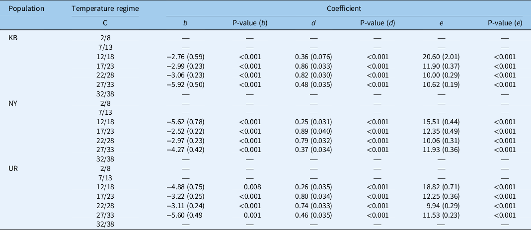
a The time-to-event-method, three-parameter Weibull equation:
 $$f\left( {t,\left( {b,d,e} \right)} \right) = d\;(\exp ( - \exp /\left[ {b\left( {\log \left( t \right) - \log \left( e \right)} \right]} \right)$$
was used, where d is maximal germination; b is the slope around the inflection point (reflecting the steepness of the curve at median germination), and e is the location parameter.
$$f\left( {t,\left( {b,d,e} \right)} \right) = d\;(\exp ( - \exp /\left[ {b\left( {\log \left( t \right) - \log \left( e \right)} \right]} \right)$$
was used, where d is maximal germination; b is the slope around the inflection point (reflecting the steepness of the curve at median germination), and e is the location parameter.
Modeling Germination Rate as a Function of Temperature
The fitted curves were used to derive the germination rates for the 10th, 15th, 20th, and 25th percentiles (GR10, GR15, GR20, and GR25), which were used to parameterize Equation 3 (Supplementary Figure S3). By regarding the percentile g as a factor and allowing different parameters for different percentiles, we reached a total number of 16 parameters. However, consistent with the literature (Bradford Reference Bradford2002; Rowse and Finch-Savage Reference Rowse and Finch-Savage2003), we tested three other modeling approaches, one with 7 parameters (Washitani Reference Washitani1987) and two with 10 parameters (Mesgaran et al. Reference Mesgaran, Onofri, Mashhadi and Cousens2017), which adjust constant cardinal temperatures for all percentiles.
The computed RMSE values were similar for all four modeling approaches, being <1%. This trend was observed for all three populations (Table 3). However, when the AIC was used, some differences were observed between the different model approaches. As Table 3 shows, the variable model (variable T b, T o, T c, and b) provided the worst fit with the highest AIC value for the Newe Ya’ar and Kibbutz Urim populations (Table 3). The computed AIC values for the Kfar Blum population were −127, −134, −121, and −121 for the variable model, fixed T c, variable T c, and variable T o approaches, respectively. The fixed T c approach provided the best fit with the lowest AIC values in all populations, with the extracted values being −136, −134, and −145 for the Kibbutz Urim, Kfar Blum, and Newe Ya’ar populations, respectively (Table 3).
Table 3. Akaike information criterion (AIC), root mean-square error (RMSE), degrees of freedom (df), and number of parameters of the four models used (reference in parentheses) to describe the relationship between germination rate (GR) and temperature of three Solanum elaeagnifolium populations (Kfar Blum [KB], Newe Ya’ar [NY], and Urim [UR]).

a T c, ceiling temperature; T o, optimum temperature; T b, base temperature.
When the computed cardinal temperatures were compared across the modeling approaches with the constant cardinal temperatures (fixed T c, variable T c, and variable T o), similar values were observed, with negligible differences of 0.01 C between them. These findings coupled with the lowest AIC value observed in the fixed T c model and the smallest number of parameters (parsimony rule) motivated us to select this model for the later stages of analysis.
When the fixed T c model was used, the three cardinal temperatures were not significantly different between the three S. elaeagnifolium populations, and overlapping 95% CIs were observed (Figure 2; Table 4). For example, the estimated T b values and their respective 95% CIs for the Kfar Blum, Newe Ya’ar, and Kibbutz Urim populations were 10.95 ± 1.31, 9.99 ± 0.45, and 10.85 ± 1.17, respectively. In addition, the b parameter decreased with the percentiles in all three populations, suggesting a higher GR in the lowest percentiles (Table 4). The values of the b parameter ranged between 0.155 to 0.117 for all populations, and for the Newe Ya’ar population, the computed values of b 10, b 15, b 20, and b 25 were 0.153, 0.141, 0.131 and 0.117, respectively.

Figure 2. Relationship between germination rates (GR) of different percentiles (g) and temperature for three Solanum elaeagnifolium populations (Kfar Blum [KB], Newe Ya’ar [NY], and Urim [UR]). Symbols show the observed data, while lines show the fitted curves (Equation 4), with the parameters of Table 4.
Table 4. Cardinal temperatures, namely, base temperature (T b), optimum temperature (T o), and ceiling temperature (T c), and maximal germination rate (GR) value (b) of the different percentiles of three Solanum elaeagnifolium populations (Kfar Blum [KB], Newe Ya’ar [NY], and Urim [UR]), their SEs (in parentheses), lower and upper 95% confidence intervals (CIs), and P-values that were estimated from the Washitani model (Washitani Reference Washitani1987) in Equation 4.

The modeling approaches used in this study take into consideration the different germination characteristics of the various percentiles within the populations. These differences were reflected by the b parameter in Equation 4, which represents the maximal value of GR (Covell et al. Reference Covell, Ellis, Roberts and Summerfield1986; Ordoñez-Salanueva et al. Reference Ordoñez-Salanueva, Seal, Pritchard, Orozco-Segovia, Canales-Martínez and Flores-Ortiz2015; Rowse and Finch-Savage Reference Rowse and Finch-Savage2003). The insight gained into the germination dynamics of different S. elaeagnifolium percentiles can facilitate optimal decision making regarding control activities. Revealing such dynamics enables control activity to be targeted to the time when most of the population has emerged and prevent early or late applications. These nonoptimal timings may result in uncontrolled germination flashes or highly developed weeds that are not adequately controlled, respectively. However, no significant differences were observed in the percentiles of the different populations, which suggests similar germination patterns.
The fixed T c model allowed accurate prediction of S. elaeagnifolium germination across the entire temperature range with a high level of accuracy (Figure 3). It takes into consideration the decreased germination rate above the optimal temperatures (22/28 C) and is thus superior to the so-called linear models that exhibit limited prediction accuracy for the optimal temperature range (Cochavi et al. Reference Cochavi, Rubin, Achdari and Eizenberg2016). These models take into consideration a wide range of temperatures (Parmoon et al. Reference Parmoon, Moosavi, Akbari and Ebadi2015) to provide a robust tool for describing weed germination dynamics for various weed species (Forcella et al. Reference Forcella, Benech Arnold, Sanchez and Ghersa2000; Mesgaran et al. Reference Mesgaran, Onofri, Mashhadi and Cousens2017). Prediction models can be employed to improve decision making regarding the nature and timing of weed control tools. For example, the results of any control tactic (e.g., herbicides, cultivation, or flaming) are affected by weed growth stage and density at the time of application (Lati et al. Reference Lati, Filin and Eizenberg2012).

Figure 3. Germination dynamics of Solanum elaeagnifolium in relation to growing degree days (GDD) using log-logistic three parameters:
 $${\rm{cumulative\;germination}}\;\left( \% \right) = d/(1 + {\rm{exp}}(b\left( {\log \left( {{\rm{GDD}}} \right) - \log \left( e \right)} \right)$$
, where d is maximal germination, b is the steepness of the curve at the inflection point, and e is the median germination GDD. The model was fit for all three populations separately, namely: (A) Kfar Blum (KB), (B) Newe Ya’ar (NY), and (C) Urim (UR); and (D) for all three populations for all the temperature regimes. The evaluated parameters (d, b, and e), the cardinal temperatures (base temperature [T
b], optimum temperature [T
o], and ceiling temperature [T
c]), P-value, and root mean-square error (RMSE) value were: d = 0.85, b = −3.06, e = 129.3, T
b = 10.82 C, T
o = 23.86 C, T
c = 35.9 C, p < 0.001, and RMSE = 0.064.
$${\rm{cumulative\;germination}}\;\left( \% \right) = d/(1 + {\rm{exp}}(b\left( {\log \left( {{\rm{GDD}}} \right) - \log \left( e \right)} \right)$$
, where d is maximal germination, b is the steepness of the curve at the inflection point, and e is the median germination GDD. The model was fit for all three populations separately, namely: (A) Kfar Blum (KB), (B) Newe Ya’ar (NY), and (C) Urim (UR); and (D) for all three populations for all the temperature regimes. The evaluated parameters (d, b, and e), the cardinal temperatures (base temperature [T
b], optimum temperature [T
o], and ceiling temperature [T
c]), P-value, and root mean-square error (RMSE) value were: d = 0.85, b = −3.06, e = 129.3, T
b = 10.82 C, T
o = 23.86 C, T
c = 35.9 C, p < 0.001, and RMSE = 0.064.
Development of the Solanum elaeagnifolium Germination Dynamics Model
To develop a thermal time model for estimating cumulative S. elaeagnifolium germination, data from all temperature regimes were combined. For each population separately, the chronological time (days) was converted to thermal time (GDD) by using Equation 6 and the computed cardinal temperatures. As Figure 3 and Table 5 show, the three-parameter log-logistic equation adequately described the germination dynamics of all S. elaeagnifolium populations, with P-values <0.001. The resulting RMSE values for all three populations were <0.07%, and the P-values for the three parameters, b, d, and e, were highly significant (P < 0.001). Furthermore, the values of the estimated parameters were similar for the three populations. The approximate difference of 10 GDD units in the value of the e for the Newe Ya’ar population is negligible, being equivalent to half a day under spring–summer temperatures (Table 5).
Table 5. Estimated parameters of the three-parameter log-logistic equation describing the germination dynamics of Solanum elaeagnifolium in relation to growing degree days (GDD):
 $$f\left( {{\rm{GDD}},\left( {b,d,e} \right)} \right) = d/(1 + {\rm{exp}}(b\left( {{\rm{log}}\left( {{\rm{GDD}}} \right) - {\rm{log}}\left( e \right)} \right)$$
, where d is maximal germination, b is the steepness of the curve at the inflection point, and e is the median germination GDD.
$$f\left( {{\rm{GDD}},\left( {b,d,e} \right)} \right) = d/(1 + {\rm{exp}}(b\left( {{\rm{log}}\left( {{\rm{GDD}}} \right) - {\rm{log}}\left( e \right)} \right)$$
, where d is maximal germination, b is the steepness of the curve at the inflection point, and e is the median germination GDD.

a RMSE, root mean-square error.
Finally, by virtue of the lack of significant differences between the S. elaeagnifolium populations in terms of cardinal temperatures and predictive models, all data were pooled. The cardinal temperatures were then re-estimated using the fixed T c model and were used for development of the prediction model. Here, the estimated cardinal temperatures were 10.82, 23.86, and 35.9 C for T b, T o, and T c, respectively. As Figure 3 shows, the log-logistic equation adequately described the germination dynamics of all three populations taken together (P < 0.001), with the RMSE value being similar, 0.064%, compared with the values computed for each population separately. These results indicate the accurate germination prediction ability offered by the cardinal temperatures that were evaluated by the fixed T c model, with the computed cardinal temperatures not being significantly different between the three populations (Table 4). They also provide support for the similarity of the germination patterns of the three examined populations, which were collected from various regions in Israel, over a250 -km range from the north (Kfar Blum) to the south (Kibbutz Urim). Despite the fact that Kibbutz Urim is located in what is considered to be an arid region, Supplementary Figure S4 shows that, in terms of temperature, Kfar Blum, Newe Ya’ar, and Kibbutz Urim share similar values and that the average temperatures between March and May (main germination period of S. elaeagnifolium) are similar. Kfar Blum has a cooler autumn–winter season (September to February) than Kibbutz Urim, with a temperature difference of approximately 4 C. Nonetheless, this difference in environmental conditions was not reflected in a lower T b, and even the 95% CIs for the temperature ranges of these two populations were similar, lying between 8 and 14 C. The lack of differences in the cardinal temperatures offers an agronomic advantage. Any decision making regarding the control of this weed that is based on these temperatures will be identical for all regions. However, the three locations do differ in amounts of precipitation, with Kibbutz Urim having significantly lower rainfall than the other two locations. As this environmental parameter plays a crucial factor in seed germination (Jami Al-Ahmadi and Kafi Reference Jami Al-Ahmadi and Kafi2007), future research will have to develop a hydrothermal germination dynamics model (Alvarado and Bradford Reference Alvarado and Bradford2002; Mesgaran et al. Reference Mesgaran, Onofri, Mashhadi and Cousens2017; Onofri et al. Reference Onofri, Benincasa, Mesgaran and Ritz2018). Such a model would be relevant for nonirrigated fields, natural reserves, and other niches where water is a limiting factor that may inhibit seed germination.
To best of our knowledge, this is the first study to estimate cardinal temperatures for S. elaeagnifolium germination. The estimated temperatures are in agreement with those for other weed species originating from the southern United States and Central America that are associated with warm and dry climates. For example, the T b value (10.82 C) revealed in our study is within the range of other typical “summer” weeds, between 7.5 C (common purslane [Portulaca oleracea L.]) and 16.9 C (Palmer amaranth [Amaranthus palmeri S. Watson]) (Cochavi et al. Reference Cochavi, Goldwasser, Horesh, Igbariya and Lati2018). Furthermore, the optimal germination temperature of 23.8 C and high ceiling temperature of 35.9 C, which are typical for the Israeli early and midsummer, respectively, can explain the adoption of this weed over wide areas in the Mediterranean region. However, our results were driven by controlled conditions, and further validation under field conditions with a varying range of temperature fluctuations are needed to ensure robustness.
In conclusion, S. elaeagnifolium is a troublesome weed that poses a threat to agricultural summer crops and natural ecological niches in Israel and other parts of the world (Boyd et al. Reference Boyd, Murray and Tyrl1984; Mekki Reference Mekki2007; Qasem et al. Reference Qasem, Al Abdallat and Hasan2019; Travlos Reference Travlos2013). Herbicide-based options to control S. elaeagnifolium are limited (Wu et al. Reference Wu, Stanton and Lemerle2016); thus, extensive biological knowledge about this weed is a prerequisite for improving its control. The main objectives of this study were therefore to determine the cardinal temperatures for the germination of this weed and to develop a prediction model for its germination. It was found that the seed germination characteristics of the three examined local S. elaeagnifolium populations were similar, including the impact of alternating temperature regimes on cumulative germination (proportion and rate) and cardinal temperatures. Solanum elaeagnifolium germination will not occur under constant temperatures, and an alternation range of ≥6 C is needed for optimal germination. The cardinal temperatures for seed germination of S. elaeagnifolium were found to be 10.8, 23.8, and 35.9 C for the base, optimal, and ceiling temperatures, respectively. These biological parameters can be used to accurately predict S. elaeagnifolium seed germination under different temperature regimes. The biological data presented here regarding the impact of temperature on S. elaeagnifolium germination can be used to improve the control of this weed through smart decision making regarding tilling, timing of weed control, and weed control tool(s).
Supplementary material
To view supplementary material for this article, please visit https://doi.org/10.1017/wsc.2022.19.
Acknowledgment
The authors wish to thank the chief scientist of the Israel Ministry of Agriculture for funding this project (grant no. 20-02-0076). The authors declare that they have no conflict of interest.


