1. INTRODUCTION
An integrated GPS/INS system can provide precise navigation solutions while GPS signals are available. The GPS solution has a consistent and long-term stable accuracy, which is used to update the INS solution. Meanwhile, the accurate short-term INS solution can be used to bridge GPS outages. The KF is typically used to fuse the measurements from the GPS and INS devices. Due to the increasing use of low-cost MEMS inertial sensors for land vehicle applications, however, the traditional KF methodology is found to be inadequate due to the poor quality of the MEMS inertial measurements. When GPS outages occur, for example in tunnels, urban canyons, or indoors, the accuracy of the navigation system will degrade sharply, as the KF cannot be updated with the GPS measurements. It is a challenge to develop an optimal real-time GPS/INS integration algorithm that can maintain required system performance during GPS outages [Reference Li, Mumford and Rizos1–Reference Goodall, El-Sheimy and Chiang4].
Combination of the KF and neural network (NN) technique is one of the widely-used methods to improve the performance of GPS/INS integrated systems, as in, for example, the NN-aided adaptive extended KF (EKF) [Reference Jwo and Huang5], the NN-tuning KF [Reference Korniyenko, Sharawi and Aloi6], the use of the NN for de-noising MEMS-based inertial data [Reference El-Rabbany and El-Diasty7], and the NN/KF hybrid approach [Reference Wang, Wang, Sinclair and Watts8]. In an NN-based integrated system, an NN is trained to map the vehicle dynamics with corresponding KF states during periods of good quality GPS data. Once the NN is trained, its output is then used to correct the INS when the GPS solution becomes unavailable.
However, it is critical to select sufficient data samples of good quality for the NN to deliver good performance. This is sometimes too rigorous a requirement which limits real world application of the NN-based methods. Furthermore, an NN-based method has some drawbacks, such as the existence of many local minimum solutions and the difficulty in choosing the number of hidden units. This paper explores the application of a new class of kernel-based techniques known as LS-SVM to aid GPS/INS integration. In contrast to the NN approaches, the SVM, which can be characterised by the convex optimisation problems, has been developed in the area of statistical learning theory and structural risk minimisation [Reference Vapnik9][Reference Vapnik10]. LS-SVM models scale very well to high dimension input spaces. Moreover, using weighted least squares and special pruning techniques, it can be employed for robust nonlinear estimation. This paper describes the LS-SVM regression algorithm and the implementation of an LS-SVM/KF hybrid method for GPS/INS integration. As with the NN approach, the LS-SVM is used to correct the INS errors during GPS outages, based on the modelling achieved from the advance training when GPS is available. Field test data is used to evaluate the performance of the proposed method and the result are compared with the more common NN-aided GPS/INS techniques.
2. INTEGRATION KALMAN FILTER
As the core of an integrated system, the integration KF must be carefully designed. A 15-state KF is used for the experiments reported in this paper, with the states listed in Table 1. The inertial measurement unit (IMU) sensor errors are the various scale factor errors, biases, non-orthogonality errors, and noise terms.
Table 1. States of the integration KF.

The INS error equation in the psi-angle form is [Reference Bar-Itzhack and Berman11]:
The sensor errors are modelled as random walk processes:
where δr, δν and δψ are the error vectors of position, velocity and angle, respectively. εa and εg are the errors of the accelerometers and gyroscopes, respectively. w a and w g are the white noises associated with the accelerometers and gyroscopes, respectively. ωie is the Earth rate vector; ωin is the angular rate vector of the navigation frame relative to the inertial frame; ωen=ωin=−ωie; and f is the specific force.
The process model of the system in Equations (1) – (5) can be also written in matrix form:
![\left[{\matrix{ {\delta \mathop r\limits^{ \bullet } } \hfill \cr {\delta \mathop v\limits^{ \bullet } } \hfill \cr {\delta \mathop \psi \limits^{ \bullet } } \hfill \cr {\mathop {\varepsilon _{a} }\limits^{ \bullet } } \hfill \cr {\mathop {\varepsilon _{g} }\limits^{ \bullet } } \hfill \cr} } \right]\ \equals \left[ {\matrix{ { \minus \omega _{en}^{ \times } } \hfill \tab \hfill I \hfill \tab \hfill 0 \hfill \tab \hfill 0 \hfill \tab \hfill 0 \hfill \cr \hfill 0 \hfill \tab \hfill { \minus \lpar \omega _{ie} \plus \omega _{in} \rpar ^{ \times } } \hfill \tab \hfill {f^{ \times } } \hfill \tab \hfill {C_{nb} } \hfill \tab \hfill 0 \hfill \cr \hfill 0 \hfill \tab \hfill 0 \hfill \tab \hfill { \minus \omega _{in}^{ \times } \ \ } \hfill \tab \hfill 0 \hfill \tab \hfill {C_{nb} } \hfill \cr \hfill 0 \hfill \tab \hfill 0 \hfill \tab \hfill 0 \hfill \tab \hfill 0 \hfill \tab \hfill 0 \hfill \cr \hfill 0 \hfill \tab \hfill 0 \hfill \tab \hfill 0 \hfill \tab \hfill 0 \hfill \tab \hfill 0 \hfill \cr} } \right]\ \left[ {\matrix{ {\delta r} \hfill \cr {\delta v} \hfill \cr {\delta \psi } \hfill \cr {\varepsilon _{a} } \hfill \cr {\varepsilon _{g} } \hfill \cr} } \right]\ \plus \left[ {\matrix{ {w_{r} } \hfill \cr {w_{v} } \hfill \cr {w_{\psi } } \hfill \cr {w_{a} } \hfill \cr {w_{g} } \hfill \cr} } \right]](https://static.cambridge.org/binary/version/id/urn:cambridge.org:id:binary:20151022065409686-0811:S0373463309990361_eqn6.gif?pub-status=live)
where the direction cosine matrix C nb implements the transformation from the body-frame coordinate system to the navigation-frame coordinate system.
The observation vectors of the KF are formed by differencing the GPS and INS positions (rgps, rins) and the velocities (vgps, vins). When GPS data is available, the observation vectors are updated with the GPS and INS measurements. However, when GPS outages occur the KF cannot be updated with the GPS measurements and the accuracy of the navigation system will degrade sharply. In the case of no more measurement correction information, it is a challenge to improve the accuracy of the INS-only navigation solution.
3. LS-SVM
LS-SVM is widely used for nonlinear estimation. The LS-SVM regression algorithm is used here to improve the accuracy of the INS-only navigation solution during GPS outages.
3.1. LS-SVM Regression Algorithm
Given a training set ![]() , the LS-SVM model for nonlinear function estimation has the following representation in the feature space [Reference Vapnik, Suykens and Vandewalle12]:
, the LS-SVM model for nonlinear function estimation has the following representation in the feature space [Reference Vapnik, Suykens and Vandewalle12]:
where the input data is x∊![]() n and the corresponding output is y∊
n and the corresponding output is y∊![]() . The nonlinear function ϕ maps the input space to a so-called higher dimensional feature space. The term b is the bias term.
. The nonlinear function ϕ maps the input space to a so-called higher dimensional feature space. The term b is the bias term.
The optimisation problem is:
subject to the equality constraints:
The cost function with squared error and regularisation corresponds to a form of ridge regression [Reference Golub and Van Loan13].
To solve the optimisation problem above, the Lagrangian function is constructed:
where αk are the Lagrange multipliers. The conditions for optimality are given by:
The solution of Equation (11), αk and b, can be computed from the input of the sample sets when the LS-SVM is trained. Applying the Mercer condition one obtains:
As a result, the LS-SVM model for nonlinear function estimation becomes:
In this paper the most universal RBF kernels are chosen as the kernel function of the LS-SVM:
Note that in the case of RBF kernels, only two additional tuning parameters, γ (regularisation parameter) and σ (kernel width), need to be selected. They need to be an optimal combination, determined before the LS-SVM is trained. There are several methods that can be used, e.g. bootstrapping [Reference Vapnik, Suykens and Vandewalle12], VC bounds statistical learning theory [Reference Vapnik9][Reference Vapnik10], genetic algorithms, and inference or Bayesian learning methods [Reference Van Gestel, Suykens, Lanckriet, Lambrechts, De Moor and Vandewalle14]. A simplified cross-validation method is developed in this paper, which defines a training set, consisting of the validation and the verification subsets. In the validation subset, the LS-SVM is trained with some empirical combinations of tuning parameters. Those combinations, which enable the output of the LS-SVM to reach the given accuracy, are selected as the primary tuning parameters. Then they are used to further train the LS-SVM with the verification set, and the final selection of tuning parameters is made. In addition, system modelling is performed along with the process of selection of tuning parameters so that the system model is also obtained. A well-trained LS-SVM can be used in many physical scenarios for different definitions of the input/output.
3.2. The Input/Output Design of LS-SVM
A KF state's variation with time is mainly caused by vehicle dynamics (changes of vehicle velocity and attitude). It has been found that there is a relatively high correlation between vehicle dynamics and some KF states, in particular the velocity and attitude errors and the horizontal accelerometer biases [Reference Wang, Wang, Sinclair and Watts8]. It is difficult to model this correlation, but it could be mapped by a properly designed LS-SVM after adequate training. When the GPS data is unavailable, with the input of vehicle dynamics information the LS-SVM outputs the prediction of the KF states, which are used to compensate the INS solution (as the integration KF does when the GPS data is available).
The dynamic variations are selected as the input of the LS-SVM and the KF states are selected as the output. For land vehicle applications, vertical movement can be ignored and the input of the LS-SVM can be selected as:
To reduce the computational load, only the KF states that have a major impact on the accuracy of the navigation solutions will be selected as the output of the LS-SVM. The simulation results show that δν and δψ are the most significant factors. The quality of the solution with just δν and δψ updated is very close to that when all states (except δr) are updated. Therefore the output of the LS-SVM can be simplified as:
The structure of input and output is consistently implemented for the training and prediction stages.
4. LS-SVM AND KF HYBRID METHOD FOR GPS/INS INTEGRATION SYSTEM
With the selected input and output of the LS-SVM for GPS/INS integration, the LS-SVM/KF hybrid architecture can be designed. The hybrid method consists of two stages. The first is the LS-SVM/ KF hybrid system. The second is the LS-SVM-based prediction during GPS outages.
4.1. LS-SVM and KF Hybrid Architecture for GPS/INS Integration System
When GPS data is available the LS-SVM functions in the training mode. The configuration of the LS-SVM/KF hybrid system for GPS/INS integration is illustrated in Figure 1. The vehicle's dynamics are derived from the navigation solution and continuously input to the LS-SVM for training. The KF estimates of δν and δψ are introduced into the LS-SVM as the target vectors of the training. The observation vectors of the KF are formed by differencing the GPS and INS positions (rgps, rins) and the velocities (vgps, vins).
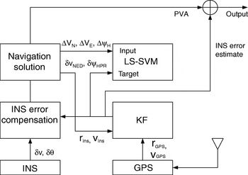
Figure 1. Configuration of the LS-SVM/ KF hybrid system.
4.2. Configuration of the LS-SVM-based prediction during GPS outages
Without updating by GPS the KF estimates remain unchanged from the values at the last epoch before the GPS outage. The integrated system actually becomes simply a stand-alone INS. Figure 2 illustrates the configuration of the LS-SVM-based prediction during a GPS outage. The LS-SVM functions in the prediction mode, in which the output of the LS-SVM is used for error compensation. The vehicle dynamics derived from the navigation solution are continuously input into the LS-SVM, as was done during the training phase.

Figure 2. Configuration of the LS-SVM-based prediction during GPS outages.
5. TEST
A low-cost FPGA-based GPS/INS integration system was utilised to collect field test data in order to evaluate the performance of the proposed method. The hardware components of the system included Boeing's C-MIGITS II IMU, an OmniStar GPS receiver, and an FPGA device built on the Nios II soft-core processor [Reference Li, Mumford and Rizos1][Reference Li, Mumford and Rizos15]. The C-MIGITS II has a gyro bias of about 30 deg/hr and an accelerometer bias of approximately 4 mg [16]. It can output the inertial data (delta velocity and delta theta) for subsequent processing. The trajectory of the test is shown in Figure 3, where four 30-second simulated GPS outages are marked by red lines.

Figure 3. Trajectory of the vehicle in the field test.
5.1. LS-SVM Training
Two independent sets of 100 epoch sample vectors were utilised to train the LS-SVM. The first set was used for the validation, in which the LS-SVM was trained with nine combinations of empirical σ and γ. The parameter e was chosen as 10−2, which is related to the accuracy of the model fitting. The velocity and attitude errors are the output of the LS-SVM. The training results are listed in Table 2, where the tests 4–7 were selected as the primary tuning parameters, which were to be used to further train the LS-SVM with the verification set, and the results are listed in Table 3. From Table 3, σ=50 and γ=1000 were the final selection of tuning parameters. Finally, using both the validation and verification sets as well as the selected tuning parameters, the LS-SVM was trained again to obtain the system model.
Table 2. LS-SVM training results with the validation set.
Table 3. LS-SVM training results with verification set.

5.2. Prediction and Analyses
In order to assess the performance of the hybrid method, four 30-second GPS outages were simulated. The LS-SVM result was compared with the INS–only solution and the NN/KF hybrid solution during these outages. The back propagation (BP) NN/KF hybrid method has the same input/output as the LS-SVM. The number of the training was 5000. The activation function of the hidden layer is sigmoid. The BP NN has three neurons in the input layer and six neurons for the output layer, as well as for the 100 epoch training set. The results during the four outages are listed in Tables 4, 5 and 6, where the position, velocity and attitude errors from the INS-only, LS-SVM and NN methods are compared.
Table 4. The position errors (m) from the INS-only, NN/KF and LS-SVM/KF methods.

Table 5. The velocity errors (m/s) from the INS-only, NN/KF and LS-SVM/KF methods.

Table 6. The attitude errors (deg) from the INS-only, NN/KF and LS-SVM/KF methods.

Note that the errors for the LS-SVM/KF are smaller than the ones for the NN/KF and INS-only methods, confirming that the proposed algorithm can improve system performance. Figure 4 shows the attitude errors derived associated with the #1 GPS outage period. The INS-only solution is depicted in blue, the NN/KF solution in red, and the SVM/KF solution in green.

Figure 4. The attitude errors (deg) for the INS-only, NN/KF and LS-SVM/KF methods.
It is evident from Figure 4 that both the LS-SVM/KF and NN/KF can reduce the attitude errors, and that the LS-SVM/KF solution has the smallest error. Although before epoch 184906 the error of the LS-SVM solution sometimes is slightly larger than that of the NN/KF solution, the LS-SVM/KF always has smaller errors than the NN/KF after that epoch. The improvement is particularly obvious in the last segment of the period. The result shows that the proposed hybrid method is very effective as it decreases the attitude errors by about 40% and the position errors by about 20%.
To more clearly demonstrate how the proposed algorithm improves the accuracy of the solution, a 15-second GPS outage is assumed from 184920 sec to 184934 sec. The errors compensated with the prediction of the LS-SVM are shown in Figures 5, 6 and 7, where the position, velocity and attitude errors derived from the INS-only (in blue) and the LS-SVM/KF (in red) methods are compared. In those figures one can see that when the length of the GPS outage is shortened from 30 s to 15 s, the error of the LS-SVM/KF hybrid is much closer to zero than that of the INS-only, which indicates that the short-period prediction of the LS-SVM/KF has a higher accuracy than the long-period prediction. From these 15-second GPS outage results it can be seen that the proposed hybrid method decreases by about 96% the position errors, 87% the velocity errors and 81% the attitude errors.

Figure 5. The position errors (m) for the INS-only and LS-SVM/KF methods.

Figure 6. The velocity errors (m/s) for the INS-only and LS-SVM/KF methods.

Figure 7. The attitude errors (deg) for the INS-only and LS-SVM/KF methods.
6. CONCLUDING REMARKS
The principles of the LS-SVM and KF hybrid method are described and implemented in an integrated GPS/INS system. The input and output of an LS-SVM are selected on the basis of correlations between the dynamic variations and the KF states. Once the LS-SVM is properly trained in the training phase, its prediction can be used to correct the INS solution during GPS outages. Field test data is used to evaluate the performance of the proposed method. The LS-SVM results show an improved overall performance in comparison with the results of the NN and the INS-only solutions. The short-period prediction of the LS-SVM/KF has a higher accuracy than the long-period prediction. Further research is required in order to determine the relationship between the prediction accuracy and the outage length, to model the error behaviour and its relationship with the number of samples used for training, and to investigate the appropriate selection of parameters for the LS-SVM/KF prediction.