Introduction
Most bivalves are filter feeders that can contribute to creating, modifying and maintaining the surrounding habitat by acting as ecosystem engineers (Dame, Reference Dame, Kennish and Lutz1996; Philippart et al., Reference Philippart, Beukema, Cadée, Dekker, Goedhart, van Iperen, Leopold and Herman2007). Hence, they are an important component of estuarine and coastal ecosystems as they contribute to biodiversity and ecosystem functioning. In addition, due to their wide geographic and bathymetric distribution, bivalves are exposed to different environmental conditions that influence the species' life history traits (Gosling, Reference Gosling2015). Depending on the magnitude and seasonality of a changing environment, the maintenance of metabolic cost in benthic invertebrates may vary significantly (Brey, Reference Brey2001), and may influence the energy diverted to reproduction (Clarke, Reference Clarke1987). Thus, investigating the variations in reproductive processes in bivalves can enable a better understanding of population dynamics (Brey, Reference Brey2001; Cardoso et al., Reference Cardoso, Witte and van der Veer2009a) and forecast the potential of a species to acclimatize to a changing environment (Poloczanska et al., Reference Poloczanska, Babcock, Butler, Hobday, Hoegh-Guldberg, Kunz, Matear, Milton, Okey and Richardson2007; Morgan et al., Reference Morgan, O’ Riordan and Culloty2013; Ehrlén & Morris, Reference Ehrlén and Morris2015).
Different reproductive strategies among bivalve populations have been documented depending on the latitudinal gradient (Cardoso et al., Reference Cardoso, Witte and van der Veer2007; Santos et al., Reference Santos, Cardoso, Carvalho, Luttikhuizen and van der Veer2011; Verdelhos et al., Reference Verdelhos, Cardoso, Dolbeth and Pardal2011) and on local environmental conditions (Sebens, Reference Sebens1987; Sola, Reference Sola1997; Verdelhos et al., Reference Verdelhos, Cardoso, Dolbeth and Pardal2011; Magalhães et al., Reference Magalhães, Freitas and de Montaudouin2016). For instance, earlier spawning events (Philippart et al., Reference Philippart, van Aken, Beukema, Bos, Cadée and Dekker2003; Drent, Reference Drent2004; Gam et al., Reference Gam, de Montaudouin and Bazairi2010) or a decrease in reproductive investment (Pörtner & Farrell, Reference Pörtner and Farrell2008; Sokolova et al., Reference Sokolova, Frederick, Bagwe, Lannig and Sukhotin2012) and output (MacDonald & Thompson, Reference MacDonald and Thompson1986; Philippart et al., Reference Philippart, van Aken, Beukema, Bos, Cadée and Dekker2003) may occur as a result of increasing temperatures.
Traditionally, the most widely applied methods for assessing the reproductive cycle in bivalves have been histological sectioning and squash preparations of gonads. These methods, though time-consuming, are advantageous for determining the percentages of maturation stages constituting the gonads and identifying stages of development (Gosling, Reference Gosling2003). Other methods quantifying the proportion of gonadal weight with respect to body mass (gonadosomatic index) (Cardoso et al., Reference Cardoso, Witte and van der Veer2009a; Santos et al., Reference Santos, Cardoso, Carvalho, Luttikhuizen and van der Veer2011) are used as a measure of reproductive effort to determine the main gametogenic events.
The smooth clam Callista chione (Linnaeus, 1758) is a marine venerid bivalve inhabiting the soft sea beds of Atlantic and Mediterranean coastal areas (Poppe & Goto, Reference Poppe and Goto1993). In many Mediterranean countries, this species is commercially harvested by dredging boats (Tirado et al., Reference Tirado, Salas and López2002; Ramón et al., Reference Ramón, Cano, Peña and Campos2005) and off the shallow coasts of the eastern Adriatic and Greece, it is also collected by skin or scuba-diving (Metaxatos, Reference Metaxatos2004; Ezgeta-Balić et al., Reference Ezgeta-Balić, Peharda, Richardson, Kuzmanić, Vrgoč and Isajlović2011). Callista chione is a moderately long-lived bivalve with a longevity of over four decades (Ezgeta-Balić et al., Reference Ezgeta-Balić, Peharda, Richardson, Kuzmanić, Vrgoč and Isajlović2011), thereby sustainable management of its fisheries needs to be implemented to protect natural beds and secure long-term exploitation. Because of the commercial interest in this species, the reproductive cycle of C. chione has been described previously for the Atlantic (Moura et al., Reference Moura, Gaspar and Monteiro2008) and Mediterranean populations (Valli et al., Reference Valli, Bidoli and Marussi1983, Reference Valli, Marsich and Marsich1994; Tirado et al., Reference Tirado, Salas and López2002; Metaxatos, Reference Metaxatos2004; Galimany et al., Reference Galimany, Baeta, Durfort, Lleonart and Ramón2015), demonstrating variability in the timing and duration of spawning over large spatial scales. However, these studies did not assess the quantitative allocation of energy into reproduction with regard to environmental factors and were conducted only on a single population during one breeding season. Since differences in the growth rates of two relatively nearby populations of C. chione have been described previously in the eastern Adriatic (Ezgeta-Balić et al., Reference Ezgeta-Balić, Peharda, Richardson, Kuzmanić, Vrgoč and Isajlović2011), this is an ideal experimental scenario for studies on variations in the reproductive cycle in natural populations.
The main goal of this study was to investigate the relationship between temperature and reproductive cycle, body mass index, reproductive investment (in terms of gonadal mass), reproductive output (amount of gametes released into the environment) and fecundity (as weight loss at spawning) of a commercially and ecologically important species, Callista chione, sampled from two locations having known different shell growth rates (Ezgeta-Balić et al., Reference Ezgeta-Balić, Peharda, Richardson, Kuzmanić, Vrgoč and Isajlović2011). The study period also included one of the hottest summers on record since 1880, in 2015, according to the NOAA dataset (NERC, 2015). Thus, this research will also contribute to estimating the potential changes in bivalve reproductive cycles as a result of climate oscillation in the natural environment, and will provide valuable information for the management of this benthic suspension feeder.
Materials and methods
Field collection
Sampling was conducted by scuba and skin diving at two sites along the eastern Adriatic coast, Pag (44.46167°N 15.02667°E) and Cetina (43.43694°N 16.68722°E), at depths between 2 and 5 m (Figure 1). These two sites were chosen on the basis of previous studies looking at the distribution (Peharda et al., Reference Peharda, Ezgeta-Balić, Vrgoč, Isajlović and Bogner2010) and growth of this species (Ezgeta-Balić et al., Reference Ezgeta-Balić, Peharda, Richardson, Kuzmanić, Vrgoč and Isajlović2011), as it is known that these populations are characterized by different growth rates. Seawater temperature was measured hourly by data loggers (Tinytag, Gemini®) deployed at 5 and 3 m (Pag and Cetina, respectively) during the entire sampling period. Monthly precipitation data for Pag and Split meteorological stations were obtained from the Meteorological and Hydrological Service of the Republic of Croatia. A maximum of 40 standard-sized individuals (~60–75 mm in shell length) were collected monthly between July 2014 and October 2015 and transported live to the laboratory. Prior to analysis, morphometric measurements of each individual were taken for shell length (anterior-posterior axis), height (dorsal-ventral axis) and width (lateral axes) to the nearest 0.1 mm with Vernier callipers and weighed when dry, to the nearest 0.01 g.
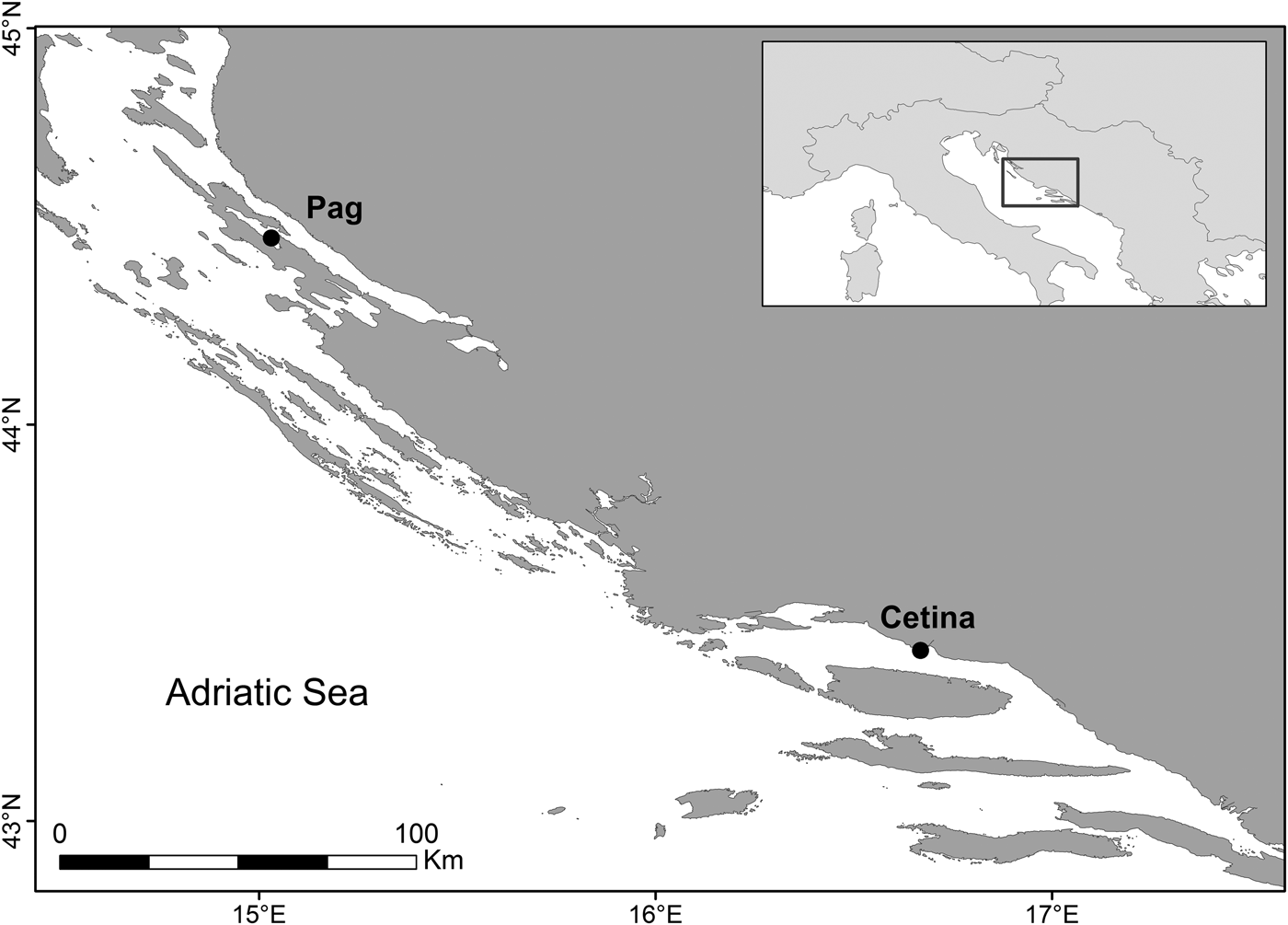
Fig. 1. Sampling locations of populations of Callista chione in the eastern Adriatic Sea: Pag (Island of Pag) and Cetina (next to Cetina River mouth).
Samples for histological analysis were collected between July 2014 and July 2015. The intended collection of a minimum of 20 individuals per month was not possible throughout the entire sampling period, and fewer individuals were collected from the Cetina site in November 2014 (N = 15), December 2014 (N = 10) and March 2015 (N = 15), and from the Pag site in January 2015 (N = 10). A total of 465 individuals were collected for this analysis; 245 from the Pag site, and 220 from the Cetina site.
Sampling for GSI analysis continued through to October 2015. It was not possible to collect 20 individuals in each month and fewer individuals were collected at the Cetina site in November 2014 (N = 10) and May 2015 (N = 19), and at the Pag site in January (N = 15), September (N = 7) and October (N = 0) in 2015. After collection, samples were stored at 5°C and processed within 24 h of collection. A total of 591 individuals were processed for this analysis and 5 (0.85%) were discarded due to accidental handling.
Histological analysis of gonad tissue
Within 3 h of collection, bivalves were opened, a piece of gonad tissue dissected, fixed in 4% formaldehyde and stored for later laboratory analysis. Samples were processed following routine histological procedures. Histological sections were examined at 100× and 400× magnification using a Zeiss Axio Lab. A1 microscope, sexually identified and assigned to a descriptive gonad developmental stage. Stages were adopted and modified from Valli et al. (Reference Valli, Bidoli and Marussi1983) and Galimany et al. (Reference Galimany, Baeta, Durfort, Lleonart and Ramón2015), and described as early active (3), late development (4), ripe (5), spawning (2) and spent/inactive stage (1). Gonadal maturation stages, scored on a scale of 1–5 for each sex, were determined based on the size of gonadal acini, presence of interstitial tissue and density and prevailing stage of germ cells. When an individual presented intermediate phases between two described stages, it was assigned to the phase dominating the greatest part of the gonads. A detailed description of each stage is given in Table 1. A total of seven samples (Pag: 4; Cetina: 3) were excluded from stage determination due to mistakes with histological procedures.
Table 1. Description of the main developmental stages described for Callista chione (adopted from Valli et al., Reference Valli, Bidoli and Marussi1983)

The mean gonad index (MGI) was calculated separately for males and females by multiplying the number of individuals in each developmental stage by the numerical ranking assigned to that stage and dividing it by the total number of individuals in each sampling month (Gosling, Reference Gosling2003).
Gonadosomatic Index
Bivalves were opened and gonads were carefully separated from the somatic tissue, and both parts were placed in previously weighed porcelain dishes. Samples were oven dried at 60°C for 48 h and weighed to obtain the estimated somatic mass index (SMI) and the gonadal mass index (GMI). These indices were calculated as the dry weight of each part (soma and gonads) divided by the cubic shell dimensions expressed as mg cm−3. To determine the relative investment in reproduction, the gonadosomatic index (GSI) was calculated as the gonadal dry mass (g) divided by the total body dry mass (g). Additionally, the body mass index (BMI), determined as the sum of the SMI and GMI, was used as a measure of body condition index. Reproductive output was also analysed as the percentage of gametes released into the environment (calculated as the relationship between gonadal mass weight and total body mass weight just before the start of the spawning season) and fecundity as the difference in gonadal mass before and after spawning, as an indication of the potential capability of an organism to produce reproductive units.
Statistical analysis
All statistical analyses were carried out using the software package Rstudio (R Core Team, 2015). For sex-ratio analysis, the χ 2 test was applied considering an expected ratio of 1:1. Levene's test was used to check for homogeneity of variances prior to any ANOVA or ANCOVA tests, and normality of residuals was assessed by the Shapiro test. A two-way ANOVA was performed to test for differences between sex and shell length during the sample period and also to test for seasonality of GSI and BMI between populations. These values were square root transformed to obtain normality and used to test for these indices. To test for sex differences in MGI, the synchronicity between GSI and BMI, and the influence of temperature on BMI and GSI, linear regression analysis using Pearson's correlation was performed for each site. Differences in gonadal mass and GSI during months previous to spawning between sites were tested using one-way ANCOVA controlling for shell length.
Results
Temperature data
Temporal oscillations in temperature followed a similar trend between sites, with monthly mean maxima of 25.1°C (Pag) and 26.4°C (Cetina) in August 2015, and maxima exceeding 28°C at both sites. Monthly mean minimum temperatures differed by ~4°C between sites, and were recorded in February 2015, 8.9°C (Pag) and March 2015, 12.7°C (Cetina). The lowest temperatures were 7.4°C (Pag) and 10.9°C (Cetina), indicating a temperature range at both sites of 21.2°C and 17.6°C, respectively. It is important to highlight that the maximum mean temperatures recorded during the two consecutive years were higher in 2015 than in 2014 by 1°C (Pag) and nearly 2°C (Cetina) (i.e. in August 2014, 24.1°C and 24.6°C, respectively).
Histological analysis
Gametogenic cycle
Histology specimens from Pag and Cetina had a mean shell length of 67.8 ± 4.7 mm and 64.7 ± 5.7 mm, respectively. There were no significant differences in shell length between males and females with respect to sampling site (two-way ANOVA F = 2.278, P = 0.133 in Pag and F = 0.251, P = 0.617 in Cetina). The population sex structure at the Pag site was 133 males (54.3%), 105 females (42.9%) and 7 hermaphrodites (2.8%), and at the Cetina site was 116 males (52.7%), 97 females (44.1%), 3 hermaphrodites (1.4%) and 4 sexually undifferentiated (1.8%). The sex ratio did not differ significantly from 1:1 (Pag: χ 2 = 3.294, P = 0.069; Cetina: χ 2 = 1.695, P = 0.193). The resulting histological sections showing the main characteristics of female and male gonad developmental stages (given in Table 1) are shown in Figure 2. Hermaphroditic samples are shown in Figure 3.
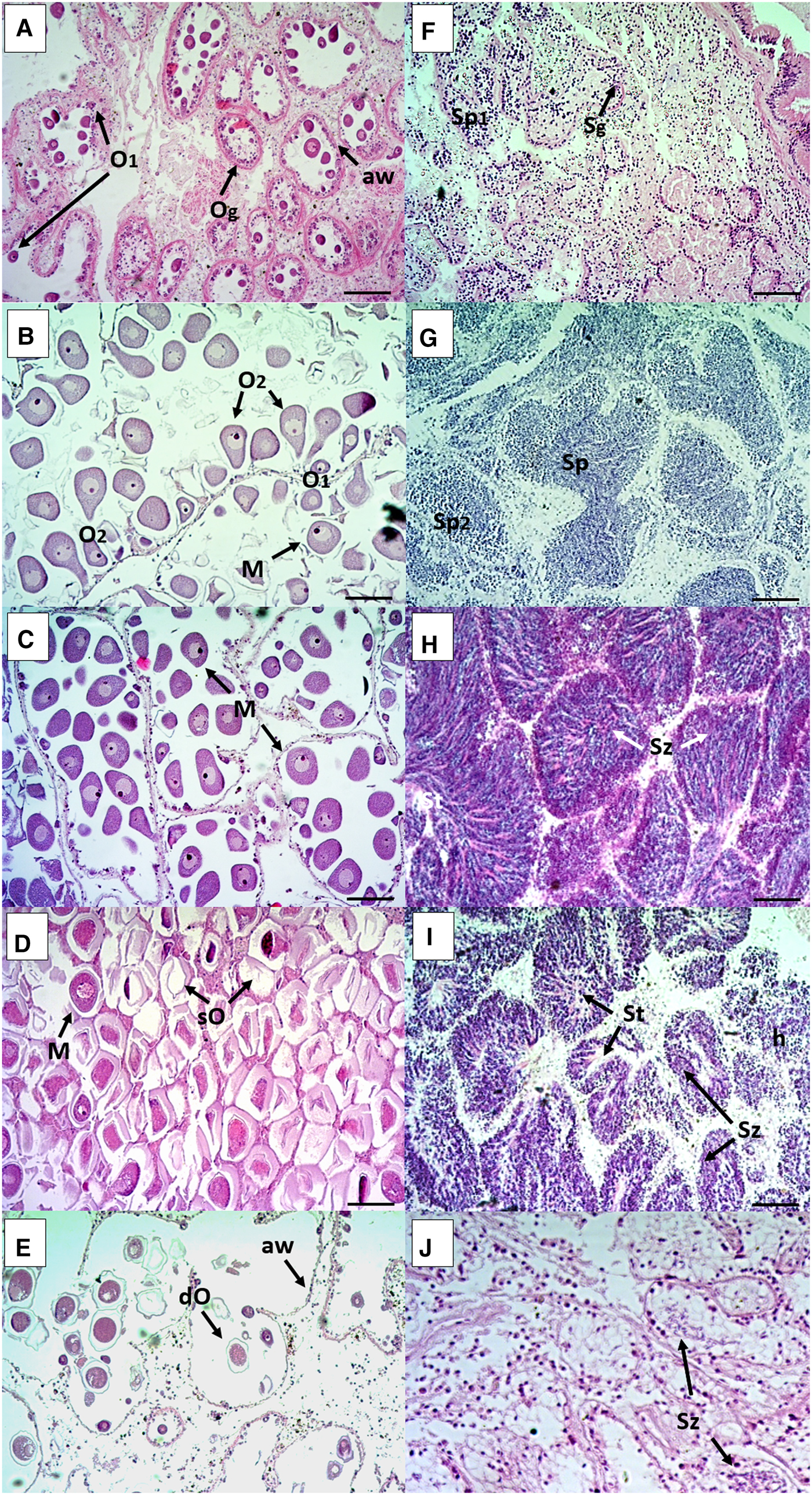
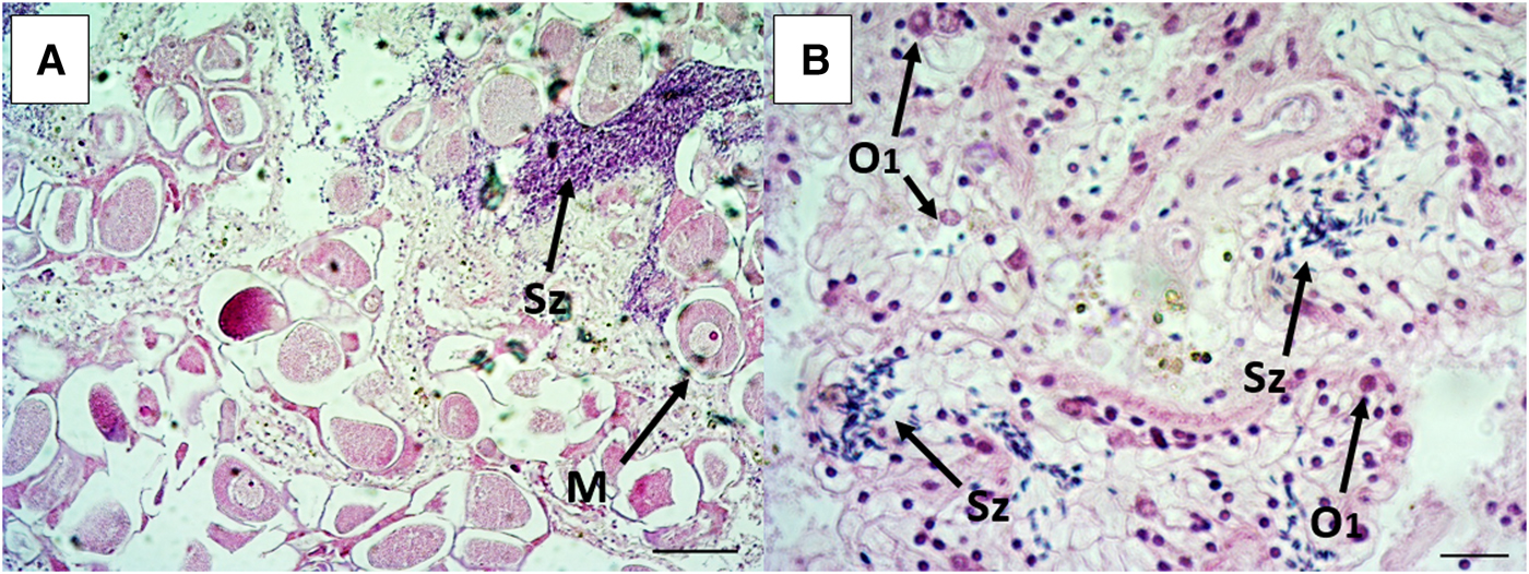
Fig. 2. Photomicrographs of the histological sections of female (left) and male (right) gonads of Callista chione characterizing each stage of gonadal maturity: (A, F) early active, (B, G) late development, (C, H) ripe, (D, I) spawning and (E, J) spent/inactive. Scale bar 100 µm. Og, oogonia; O1, primary oocytes; O2, secondary oocytes; M, mature oocytes; sO, spawned oocytes; dO, degenerative oocyte under resorption; aw, acinus wall; Sg, spermatogonia; Sp1, primary spermatocyte; Sp2, secondary spermatocyte; Sz, sperm cells; St, Sperm tails; h, haematocytes.

Fig. 3. Two hermaphrodite individuals of Callista chione shown at different magnifications and stages. A spawned individual with both free oocyte and spermatocytes (A), scale bar 100 µm. A spent to early stage with new acini walls and development of oogonia and primary oocytes as well as free sperm cells under reabsorption (B), scale bar 20 µm. O1: primary oocytes, M: mature oocytes, Sz: sperm cells.
The monthly relative frequencies of gonadal developmental stages estimated the reproductive cycle at each site (Figure 4). Overall, Callista chione was determined to be sexually active during most of the year at both study sites. The main spawning peak representing the end of gametogenesis took place earlier at Cetina (May/June 2015) than at Pag (July 2015).
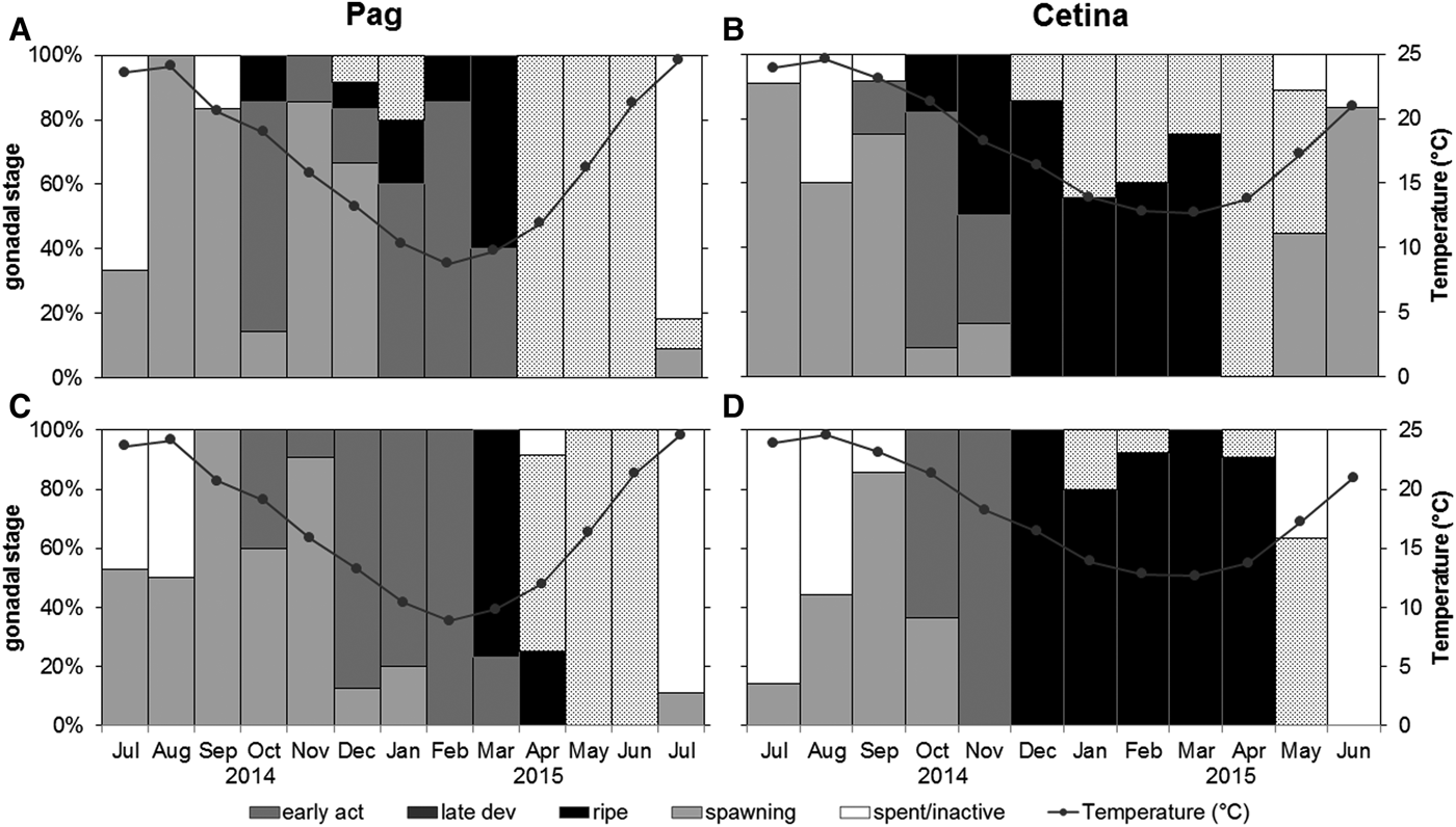
Fig. 4. Monthly relative frequencies of gonadal developmental stages of Callista chione and mean monthly temperature at Pag and Cetina sampling sites (A, B) females, (C, D) males.
The main period of gamete release at Pag started at ~12°C and extended over 4 months from April until July 2015, accompanied by increasing temperatures (Figure 4A, C). The spawning peak occurred in July 2015, coinciding with the highest temperatures in the area (>24°C). In October 2014, around 15% of females were in the ripe stage which may have led to the small spawning peak observed during December 2014 and January 2015. Consequently, four different gonadal stages were identified in December 2014. Individuals from the Pag population were in early active and late development stages for a longer period, and there was just a small transition to a ripe stage prior to spawning.
Spawning allocation in the Cetina population began in January 2015 (particularly in females) at ~14°C, at the time with the lowest mean temperature (12.7°C). The main spawning event was identified between May and June 2015, coupled with increasing temperatures (Figure 4B, D). Interestingly, females were slightly advanced in terms of gonadal development stages and had a higher percentage of spawning individuals (Figure 4B). Likewise, the spent/inactive stage was barely identified for females and those with gonads at the end of the spawning period were represented by an early active stage in more than 80% of samples. Regardless of sex, the population remained in a ripe stage for a long period during winter and early spring.
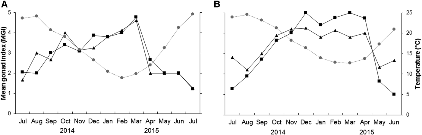
The spent/inactive stages lasted somewhat longer at Pag and in males from Cetina than in females from Cetina. Also, specimens analysed from Pag had a more synchronous cycle. The end of gametogenesis and start of a new reproductive cycle was identified for two consecutive years coinciding with the high temperature peaks in July 2014 and June/July 2015. These results were best correlated with the mean gonad index values (Figure 5).

Fig. 5. Mean monthly gonad index values of Callista chione and mean monthly temperature (grey circles); males (squares), females (triangles) from (A) Pag and (B) Cetina.
Mean gonad index
The mean gonad index (MGI) indicated that despite the slight advancement of gonadal stage in females during certain periods, both female and male cycles showed highly significant synchronicity at both sites (Pag: r = 0.86, P < 0.001; Cetina: r = 0.88, P < 0.001) (Figure 5). The highest MGI values, indicating when gonads were ripest, were identified between January and March 2015 (excluding the small peak observed in October 2014) at Pag, and between December 2014 and April 2015 at Cetina, when temperatures were at their lowest. Conversely, the release of gametes was coupled with increase in temperatures where the lowest MGI values coincided with the highest mean temperatures at both sites during two consecutive years (Figure 5).
Gonadosomatic index
GSI analysis specimens had a mean shell length of 64.0 ± 3.8 mm at Pag and 61.6 ± 2.9 mm at Cetina. All individuals were sexually mature (based on shell length ranges). The decrease in GSI indicated the timing of spawning.
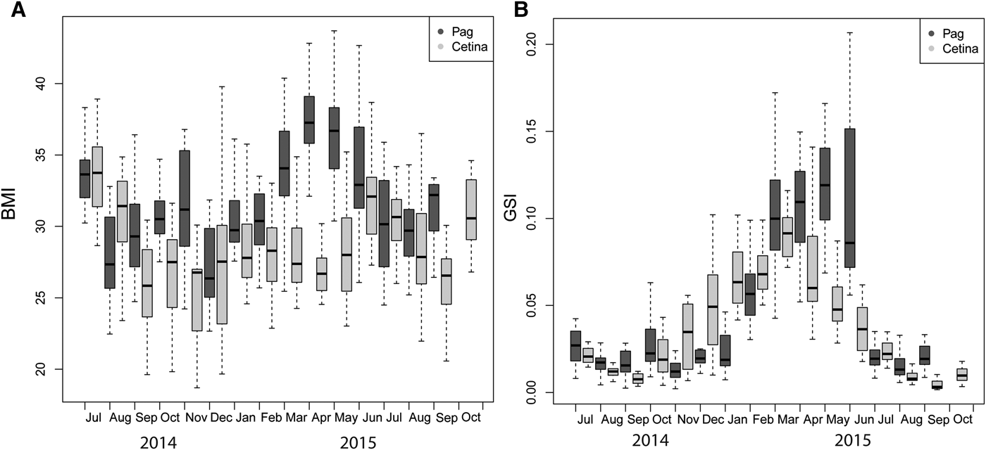
The body mass index (BMI) was determined to better understand temporal patterns in GSI and the reproductive investment for each population. BMI values of Pag specimens (31.86 ± 4.64) were significantly higher than those from Cetina (28.73 ± 4.22) (Mann–Whitney P < 0.001). The largest mean BMI values were 37.94 and 36.42 in Pag (April and May 2015) and 33.56 and 30.95 in Cetina (July 2014 and June 2015). Overall, the BMI showed a higher amplitude at Pag and smaller ranges at Cetina (Figure 6A).

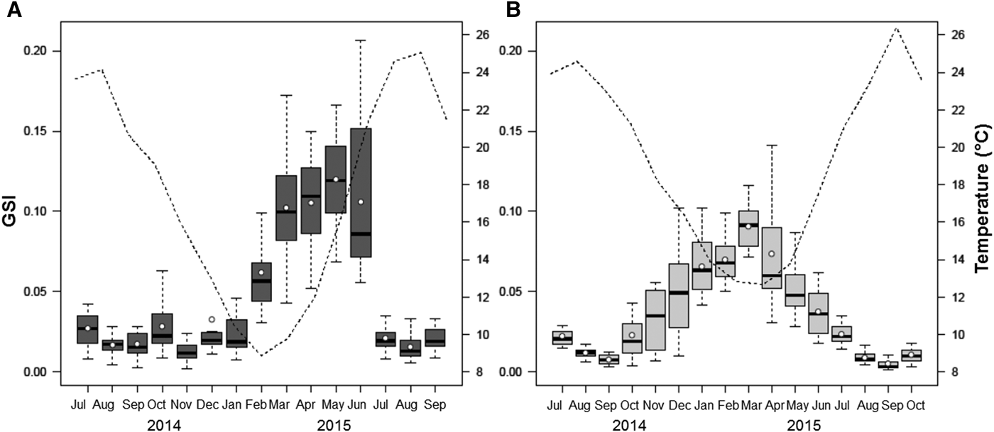
Fig. 6. Seasonal variation in body mass index (BMI) (A) and gonadosomatic index (GSI) (B) of Callista chione for the Pag and Cetina populations. Horizontal bars indicate the median value, boxes span the interquartile range – where 50% of the values fall – and discontinuous whiskers represent the data range excluding the outliers.
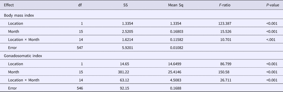
Similarly, GSI values from Pag (0.050 ± 0.046) were significantly greater than those from Cetina (0.037 ± 0.031) (Mann–Whitney P < 0.001) (Figure 6B). The combination of both indices showed a positive correlation (r = 0.77, P < 0.001) at Pag, indicating temporal synchronicity. However, the same pattern was not observed at Cetina (r = 0.13, P > 0.05), where the highest BMI values corresponded to low GSI values. There were statistically significant differences in BMI and GSI values between sites, month and their interaction, thus confirming the different spatial and temporal timing of events (Table 2).
Table 2. Analysis of variance for comparison of the body mass index and gonadosomatic index between two populations of Callista chione

Month was a considered continuous variable during the total duration of the sample period; ***P < 0.001.
At Pag, GSI started to increase in late winter/early spring and reached a peak in June 2015, with steady values throughout the spring. Gonadal investment in the Pag population reached its maximum along with the increasing temperatures and persisted for several months. Regardless of the small peak observed in October 2014, the marked drop in July 2015 identified the main spawning event, at temperatures between 21 and 24°C. A resting stage was reached nearly immediately following (August 2015), and coincided with the highest annual temperatures. A positive correlation was obtained between temperature and mean GSI, though was not statistically significant (r = 0.45, P > 0.05) (Figure 7A).

Fig. 7. Relationship between seasonal variation in the gonadosomatic index (GSI) of Callista chione and mean monthly temperature (dashed line) for populations at Pag (A) and Cetina (B). White circles and horizontal bars indicate mean and median values respectively; boxes span the interquartile range, where 50% of the values fall, and discontinuous whiskers represent the data range excluding the outliers.
At Cetina, increasing GSI values were observed during the winter months and achieved their maximum in early spring (March 2015), when the lowest mean monthly temperatures were recorded (12.7°C). Spawning took place as a series of consecutive events, indicating the liberation of gametes in different pulses during late spring and summer, reaching a nearly complete resting stage in September, and this pattern was observed in the two consecutive years. The start of a new gametogenic cycle took place in late summer/early autumn and coincided with the maximum annual temperatures. The GSI at Cetina was strongly and negatively correlated to temperature (r = −0.95, P < 0.001) (Figure 7B). Whereas temperature did not influence spawning events in the same way at both sites, the start of gametogenesis coincided with the decrease of temperatures at both locations, and was seen in both years. GSI was characterized by a unimodal distribution.
Reproductive investment, output and fecundity
Seasonal changes in gonadal mass weight were present in both populations. During the ripest stages prior to spawning, the highest gonadal production was observed at Pag with a mean weight of 348 ± 13 mg, as opposed to 165 ± 6.70 mg at Cetina. The observed differences were statistically significant between sites (ANOVA, F = 168.5, P < 0.001) and shell length did not significantly influence this variation in the response variable (ANCOVA, F = 0.587, P > 0.05), indicating a higher reproductive investment in Pag. The maximum recorded gonadal occupation in this period was 699 mg (Pag) and 311 mg (Cetina).
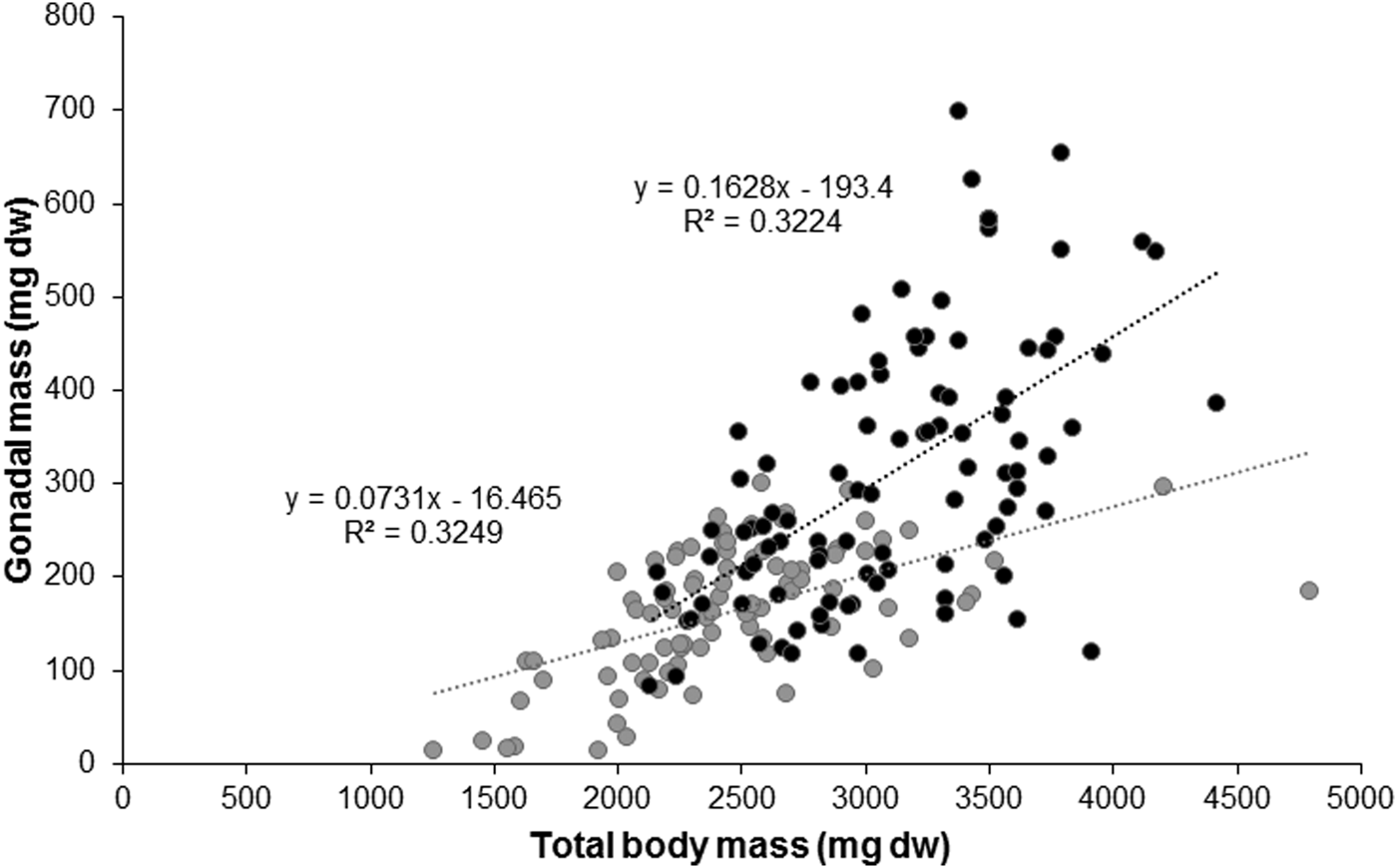
The linear relationship between gonadal mass and total body mass from individuals with highly developed gonads (mature stages) was also significant (r = 0.57, P < 0.001) (Figure 8). Gonads represented 16% of the total body mass in the Pag population, and ~7% in the Cetina population in the months preceding gamete release. At maturity, maximum gonadal mass weight % at Pag was 20.7% and reached a mean value of 2.1% after spawning, implying a drop of up to 18% and representing a loss of gonadal mass of about 260 mg. At Cetina, GSI increased up to 12.2% in March 2015 and reached a mean value of 0.9% after spawning, a drop of up to 11% and an accumulated loss of about 160 mg (considering the continuous spawning events) (see Figure 7). Therefore, a difference in reproductive output was observed between sites and showed similar results for two consecutive years, being higher at Pag.

Fig. 8. Relationship between individual gonadal mass (mg dw) and individual total body mass (mg dw) before spawning in Pag (black) and Cetina (grey).
Overall, based on the mean population values, individuals at Pag released 82% of their gonads, whereas those from Cetina released nearly the complete gonadal mass (96%). In terms of fecundity per brood, and assuming an equal weight for males and females, a higher proportion of gonadal mass was invested in reproduction at Cetina, despite the higher investment and output from the Pag population (Figure 7).
Comparative analysis of methods
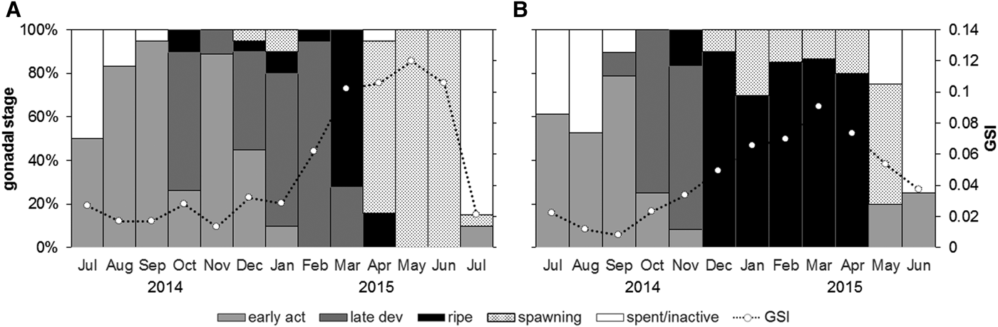
Considering the seasonal pattern of the reproductive cycle, estimations using qualitative histological analysis and gonadosomatic index yielded similar results (Figure 9). Both methodologies determined the same main spawning periods where the highest values of GSI corresponded with ripe and spawned months. Conversely, low GSI values were coupled with the spent/inactive and early developmental stages. Overall, the maximum values were obtained between March and June 2015 at Pag, and between January and May 2015 at Cetina, coinciding with the ripe/spawning stages. A transition between the last spawning event and the spent/inactive period was identified.

Fig. 9. Combination of two methodologies for determining reproductive cycle in Callista chione from the populations at Pag (A) and Cetina (B). The histogram shows the monthly relative frequencies of developmental stages for the entire population based on histological analysis and dashed line shows the temporal pattern of gonadosomatic index (GSI); white circles correspond to monthly mean GSI values.
Discussion
Reproductive cycle and temperature
Temperature and food availability are considered the main factors triggering bivalve reproduction, influencing distinct periods of the cycle (Gosling, Reference Gosling2003 and references therein). For many species, the initiation of gametogenesis is temperature dependent (Sastry & Blake, Reference Sastry and Blake1971; Bayne, Reference Bayne2009) whereas gonadal development requires nutritional input to produce mature cells (Sastry, Reference Sastry1966; Iglesias & Navarro, Reference Iglesias and Navarro1991). The complex interplay between these factors is thought to be species-dependent (Gosling, Reference Gosling2003). In the present study, a homogenous food supply between two study sites was assumed based on previous research (Purroy et al., Reference Purroy, Najdek, Isla, Župan, Thébault and Peharda2018), hence the reproductive cycle variations in the two populations of Callista chione were associated to temperature differences.
Our results on the reproductive cycle of Callista chione in the Adriatic confirmed the dioecious nature of the species and its ability to reproduce nearly year round, as observed in other Atlantic (Moura et al., Reference Moura, Gaspar and Monteiro2008) and Mediterranean populations (Valli et al., Reference Valli, Bidoli and Marussi1983, Reference Valli, Marsich and Marsich1994; Tirado et al., Reference Tirado, Salas and López2002; Metaxatos, Reference Metaxatos2004; Galimany et al., Reference Galimany, Baeta, Durfort, Lleonart and Ramón2015). In addition, an equal sex ratio was confirmed from histological analyses. Hermaphroditism was observed in the present study, as recently documented in Galimany et al. (Reference Galimany, Baeta, Durfort, Lleonart and Ramón2015), though other studies did not report them (Moura et al., Reference Moura, Gaspar and Monteiro2008) or declared them very rare (Valli et al., Reference Valli, Bidoli and Marussi1983).
In the study area, the annual temperature maxima were similar between sites, though minimum values differed by ~4°C, indicating relatively larger spatio-temporal variations, particularly at low temperatures. These inter-site temperature differences primarily influenced the onset and duration of spawning, as observed in other Mediterranean sites (Valli et al., Reference Valli, Marsich and Marsich1994; Galimany et al., Reference Galimany, Baeta, Durfort, Lleonart and Ramón2015). In both populations, gametogenesis started with the highest temperatures during two consecutive periods and reached maximum gonadal mass indices in spring. The spawning period started earlier at Cetina (in January 2015), a period with milder temperatures (~14°C) which would have favoured earlier gonad maturation, with a main spawning peak in spring followed by a gradual decrease until June/July. For this species, it is presumed that an extended spawning period is advantageous over a single event per year (Tirado et al., Reference Tirado, Salas and López2002; Moura et al., Reference Moura, Gaspar and Monteiro2008), as this also compensates for the high larval mortality (Valli et al., Reference Valli, Marsich and Marsich1994). At Pag, spawning started later, in April 2015 (~12°C), and the main peak took place during summer, with a short period of gamete release (mainly during July), indicative of major gonad storage during gametogenesis. Both spring and summer have been documented as the main spawning period in other populations of this species in the Mediterranean (Valli et al., Reference Valli, Bidoli and Marussi1983, Reference Valli, Marsich and Marsich1994; Tirado et al., Reference Tirado, Salas and López2002; Metaxatos, Reference Metaxatos2004; Galimany et al., Reference Galimany, Baeta, Durfort, Lleonart and Ramón2015) and in bivalves in general (Zwarts, Reference Zwarts1991). Synchrony was observed between the female and male reproductive cycles, which is typical of organisms with external fertilization to ensure reproductive success by increasing fertilization probabilities (Levitan, Reference Levitan1993). The highest stages of maturation were represented by high mean gonad index (MGI) values, which were inversely correlated to temperature, showing increasing values during gametogenesis and a clear drop with increasing temperatures. This correlation has previously also been described for C. chione (Galimany et al., Reference Galimany, Baeta, Durfort, Lleonart and Ramón2015) and other bivalves (Cruz et al., Reference Cruz, Rodriguez-Jaramillo and Ibarra2000; Gosling, Reference Gosling2003). Commonly, spawning takes place before highest temperatures are reached, a strategy to ensure the viability of eggs (lower during the warmest period) and to reduce metabolic demands (Honkoop & van der Meer, Reference Honkoop and van der Meer1998). The small spawning peak observed for Pag females in October 2014 could be explained by the unusual conditions in the area during that year. After a cold and rainy summer, relatively higher temperatures were recorded in that month, suggesting the high sensitivity of the species to changes in temperature and acclimatization capacity. Studies on populations with milder seawater temperatures have reported several intra-annual spawning peaks (Tirado et al., Reference Tirado, Salas and López2002; Metaxatos, Reference Metaxatos2004; Moura et al., Reference Moura, Gaspar and Monteiro2008) supporting this suggestion.
The combination of histological analysis and gonadosomatic index (GSI) revealed that both methods successfully describe the main changes in the gametogenic cycle and can be applied to assess the reproductive effort of C. chione. Microscopic examination has traditionally been used to interpret the reproductive cycle within several main gametogenic stages for different marine bivalve species including scallops, mussels and clams (e.g. Taylor, Reference Taylor and J1983; Gray et al., Reference Gray, Seed and Richardson1997; Peharda et al., Reference Peharda, Mladineo, Kekez, Bolotin, Kekez and Skaramuca2006; Delgado & Pérez-Camacho, Reference Delgado and Pérez-Camacho2007; Popović et al., Reference Popović, Mladineo, Ezgeta-Balić, Trumbić, Vrgoč and Peharda2013). Despite its advantages in determining and identifying the main stages of development during the gametogenic cycle, it is a labour-intensive method (Gosling, Reference Gosling2003). On the other hand, GSI is used to determine the storage and release of gonad material providing a quantitative estimate of gonad proportion in a short time interval (Gosling, Reference Gosling2003). As a result, GSI proved to be a reliable method for representing the main changes in the reproductive cycle, as seen in other bivalves (Royer et al., Reference Royer, Seguineau, Park, Pouvreau, Choi and Costil2008; Cardoso et al., Reference Cardoso, Witte and van der Veer2009a; Santos et al., Reference Santos, Cardoso, Carvalho, Luttikhuizen and van der Veer2011), while also allowing for determination of reproductive output and fecundity.
Body mass index
Body mass index (BMI) values were measured to recognize physiological responses to variations in environmental factors (Sebens, Reference Sebens1987; Honkoop & Beukema, Reference Honkoop and Beukema1997). Increasing BMI during the coldest period has been described in poikilotherms as a response to a reduced metabolic activity (Clarke, Reference Clarke1987; Brey, Reference Brey1995), whereas losses in BMI were enhanced by low food availability in some bivalves (e.g. Honkoop & Beukema, Reference Honkoop and Beukema1997; Cardoso et al., Reference Cardoso, Witte and van der Veer2007; Cardoso et al., Reference Cardoso, Witte and van der Veer2009b; Santos et al., Reference Santos, Cardoso, Carvalho, Luttikhuizen and van der Veer2011). In the Pag population, temporal variations in BMI increased during winter and early spring, and dropped during summer and autumn, as previously observed in this species using the condition index (CI) (Moura et al., Reference Moura, Gaspar and Monteiro2008). In this population, BMI and GSI growth were coupled and had a higher amplitude than at Cetina, indicating a higher proportional investment into soma and gonads and higher losses in body mass after spawning. In the Cetina population, the highest gonadal mass period was coupled with relatively low BMI values, followed by an increase towards the summer when spawning was taking place, suggesting a faster mass recovery and a higher investment into somatic growth rather than reproduction, as previously described for populations of Cerastoderma edule from northern Spain (Iglesias & Navarro, Reference Iglesias and Navarro1991). Therefore, using BMI or CI as indicators of gonadal development in bivalves (e.g. Gaspar & Monteiro, Reference Gaspar and Monteiro1998; Gribben et al., Reference Gribben, Helson and Jeffs2004; Drummond et al., Reference Drummond, Mulcahy and Culloty2006) needs to address temperature variations. Also, variations in food supply or salinity may mask CI results and influence the reproductive cycle (Tirado et al., Reference Tirado, Salas and López2002). Further, better somatic condition after spawning implies that once reproductive demands are satisfied, there is more energy left over for growth, as suggested for Anodonta piscinalis (Jokela & Mutikainen, Reference Jokela and Mutikainen1995). Accordingly, a higher investment into both soma and gonads in the Pag population could be at the detriment of shell growth. The observed lower shell growth rate for this population relative to Cetina (Ezgeta-Balić et al., Reference Ezgeta-Balić, Peharda, Richardson, Kuzmanić, Vrgoč and Isajlović2011) may support this possibility.
Reproductive investment, output and fecundity
The reproductive investment in bivalves has been widely studied to better interpret the allocation of energy into somatic and gonadal mass (Royer et al., Reference Royer, Seguineau, Park, Pouvreau, Choi and Costil2008; Santos et al., Reference Santos, Cardoso, Carvalho, Luttikhuizen and van der Veer2011; Velasco, Reference Velasco2013). For example, seasonal variations in gonadal mass linked to environmental conditions have been described at both the population (Brey, Reference Brey1995) and species (Jokela & Mutikainen, Reference Jokela and Mutikainen1995) levels. Such conditions may influence the constant mobilization from somatic to gonadal tissues (Valli et al., Reference Valli, Marsich and Marsich1994), resulting in different reproductive strategies as seen here. A positive relationship between gonadal mass and BMI was observed in both populations, with a higher reproductive investment at Pag (16%) than at Cetina (7%). Further, a higher percentage of gonad release with respect to the preceding state at full maturity was also observed in the Pag population, contributing to a higher reproductive output. However, in terms of fecundity, Cetina individuals had higher values (96%), indicating that most of their gonadal mass was invested in reproduction.
The presence of gonads in the resorption stage and spawning taking place during a period of high metabolic demand (summer) in the Pag population suggests the use of gonad storage as a reserve. Under unfavourable conditions, the resorption of gametes is common to subsist during periods of food scarcity, as seen in Mytilus edulis (Bayne et al., Reference Bayne, Holland, Moore, Lowe and Widdows1978) and Mya arenaria (Coe & Turner, Reference Coe and Turner1938), and may fluctuate at each gametogenic period depending on the nutritional conditions of the environment (Sastry, Reference Sastry1966; Honkoop & van der Meer, Reference Honkoop and van der Meer1998; Gosling, Reference Gosling2003). Callista chione individuals at Pag may use the energy reserves stored from the previous gametogenic cycle by gonadal resorption to ensure the generation of a new cycle, as described for Mya arenaria (Coe & Turner, Reference Coe and Turner1938). Contrarily, in Cetina individuals, gonads were most likely produced from newly available food since there was virtually no gonad mass remaining after the completion of spawning, as also seen in Cerastoderma edule populations (Cardoso et al., Reference Cardoso, Witte and van der Veer2009a).
Our studied populations experienced an increase of up to 2°C between two consecutive years with no apparent differences in their reproductive behaviour. Considering the overall greater gonadal investment at Pag and the greater weight loss during spawning at Cetina, both populations are prone to recover under short-term unfavourable changes. Small-scale studies on reproductive performance are essential to address climate oscillation issues, particularly in the management of species of commercial interest.
Conclusions
The present study demonstrated inter-site variations in the reproductive cycle of Callista chione as a result of acclimatization to different environments. Temperature is an environmental determinant influencing the timing and duration of spawning, which took place earlier in the year and lasted for a prolonged period at milder temperatures. These observations were described both from histological and gonadosomatic index analyses, which proved to be equally valid approaches in determining the main changes in the reproductive cycle. Body mass index was not a good indicator of gonadal development in this species. The reproductive investment and output were higher in the Pag population, whereas the highest fecundity was observed at Cetina. These results indicated different reproductive strategies for better acclimatization to unfavourable conditions by resorption of the gonads.
Acknowledgements
We are grateful to Mario Zokić for the collection of Cetina specimens, to graduate students for assistance in the laboratory, to Josep-Anton Sánchez for revising the statistical analysis and Linda Zanella and two anonymous reviewers for their corrections and comments that greatly improved our manuscript. This paper is dedicated to the memory of Franći Bukša.
Financial support
This work was supported by the ARAMACC Project and AP by a European Community Marie-Curie Fellowship (Call: FP7-PEOPLE-2013-ITN).