


NOMENCLATURE
- AOA
-
angle-of-attack
- AR
-
aspect ratio
- CFD
-
computational fluid dynamics
- CG
-
centre of gravity
- C L
-
lift coefficient
- C m
-
pitching moment coefficient
- FEM
-
finite element model
- L/D
-
lift-over-drag ratio
- MTOM
-
maximum take-off mass
-
 $V_s$
$V_s$
-
stall speed
- VTOL
-
vertical take-off and landing

1.0 INTRODUCTION
Vertical Take-Off and Landing (VTOL) aircraft designs have been around for several years(Reference Keane and Carr1,Reference Curtis2) . Not very long ago, helicopters represented the pinnacle of aircraft design offering a VTOL component, while fixed-wing aircraft focused on aerodynamic efficiency for longer-range transportation but requiring extensive infrastructure for take-off and landing.
Nowadays, with the increase of multi-copter designs and related advances in control and propulsion, new designs that incorporate the functional advantages of VTOL but with the improved efficiency of fixed-wing aircraft(Reference Bacchini and Cestino3,Reference Ozdemir, Aktas, Vuruskan, Dereli, Tarhan, Demirbag, Erdem, Kalaycioglu, Ozkol and Inalhan4) have emerged on the horizon. In particular, these designs have been naturally implemented in unmanned aircraft vehicles as they represent a less expensive and risky option to prove the airworthiness of the design and also provide good insight into the capabilities and shortcomings of the vehicle(Reference Ozdemir, Aktas, Vuruskan, Dereli, Tarhan, Demirbag, Erdem, Kalaycioglu, Ozkol and Inalhan4–Reference Boukoberine, Zhou and Benbouzid8).
One of the major challenges of such designs is to minimize the penalties arising from the VTOL enabling system compared with a conventional, fixed-wing design. By requiring a thrust-to-weight ratio greater than unity, this type of VTOL configuration considerably increases the required installed power and associated mass, which remains unused for most of a typical given aircraft mission(Reference Finger, Braun and Bil9).
On the other hand, the wing design is not as constrained by its low-speed performance as it would be if the VTOL capability were not available. The wing can operate near its maximum efficiency point in cruise and have a reduced area since the stall speed requirement can be higher.
Consequently, from the perspectives of energy efficiency and environmental protection, the introduction of VTOL-related penalties into a design can be overcome if the cruise segment of the mission is long enough to compensate for the initial and final energy expenditures during the take-off and landing segments.
One configuration that offers aerodynamic advantages and whose shortcomings can be overcome by the VTOL capability is the canard configuration(Reference Phillips10,Reference Selberg and Rokhsaz11) . Typically, the canard configuration has not been the first choice for aircraft designers due to its inability to generate high lift coefficients (
 $C_L$
) since, for stability reasons, the canard must stall before the wing. Another disadvantage would be the smaller vertical tail arm available, leading to wings with winglet designs and swept wings to improve lateral stability(Reference Phillips10). The aforementioned higher stall speeds potentially avoid these shortcomings because high
$C_L$
) since, for stability reasons, the canard must stall before the wing. Another disadvantage would be the smaller vertical tail arm available, leading to wings with winglet designs and swept wings to improve lateral stability(Reference Phillips10). The aforementioned higher stall speeds potentially avoid these shortcomings because high
 $C_L$
ceases to be a requirement and higher minimum operation speeds allow improved stability and authority of the vertical tail.
$C_L$
ceases to be a requirement and higher minimum operation speeds allow improved stability and authority of the vertical tail.
This work describes the design of a VTOL canard aircraft concept demonstrator for two different VTOL system implementations. The tools used in these designs are validated through experimental bench tests, and a comparison between the VTOL systems is performed. Section 2 presents the aerodynamic design procedure and the propulsion and structural sizing results. Section 3 describes the computational results obtained for the final design and the estimated performance of the considered configuration and VTOL systems. Section 4 describes the mass breakdown of a constructed prototype. The paper ends with conclusions and a summary of the findings and final remarks.
1.1 Configuration description, design and sizing
Two VTOL systems are retrofitted to a canard with pusher aircraft design to fulfil the requirements of a Maximum Take-Off Mass (MTOM) of 7kg, speed of 20m/s for cruise and 35m/s for dash as driving requirements for efficiency, and maximum power for forward flight. The first system is a symmetrical quad-rotor with a lift-and-cruise architecture; its four rotors are set up equidistant from the aircraft CG to facilitate VTOL, with an additional pusher motor for forward flight. The second system maintains the same propulsion system for forward flight, but changes the thrust distribution between the front and rear rotors, becoming an asymmetric quad-rotor, where the thrust ratio of the front to rear motors is 1:4.
It is thus easily demonstrated that, for the symmetric VTOL system, the thrust and power required is the same for all rotors, whereas the asymmetric one requires the motors closer to the CG to be more powerful.
Adding design features such as rear tilt rotor capability potentially expands the flight envelope thanks to the conversion of a significant part of the installed power into usable power for forward flight. It also couples the VTOL and forward-flight propulsion systems, thus potentially reducing the total propulsion system mass at the cost of increased design complexity. This potential mass reduction can be further improved if the rear rotors are replaced by a single rear rotor, changing the VTOL system from a quad- to tri-rotor design.
Another potentially beneficial feature would be a front rotor retraction capability for forward-flight stages, since this would probably reduce the aerodynamic drag caused by the VTOL rotors and their supporting structure.
Figure 1 depicts the four configurations analysed herein, all based on a canard-type aircraft as the baseline aerodynamic shape.
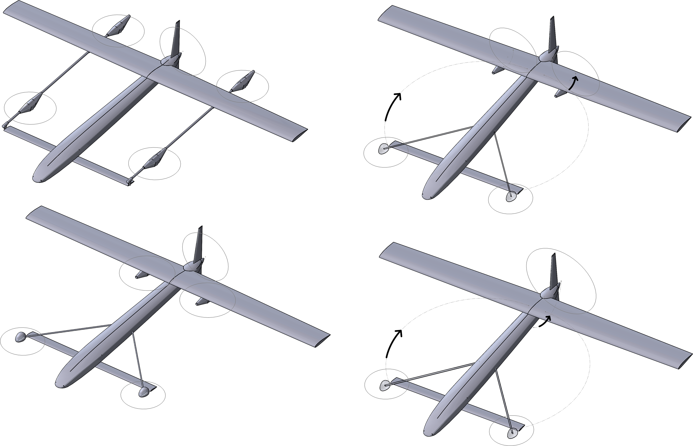
Figure 1. Configuration 1: equidistant quad-rotor (top left); configuration 2: non-equidistant quad-rotor (bottom left); configuration 3: non-equidistant tilt quad-rotor (upper right); configuration 4: non-equidistant tilt tri-rotor (bottom right). Arrows indicate retraction of the front rotors and tilt of the rear rotors for forward flight.
Configuration 1 represents an aircraft equipped with an equidistant VTOL system and a pusher motor for the forward-flight mode. The support structure for the rotors is aligned with the direction of flight for drag reduction, but the structure, motor pods and propellers are exposed to the flow at all times.
Configuration 2 represents an aircraft equipped with an asymmetric thrust VTOL system, where the front rotors are farther from the CG than the rear rotors, with a pusher motor for the forward-flight mode. The front rotors are supported by booms angled relative to the direction of flight, while the rear rotors are mounted under the wing. In this configuration also, the structure, motor pods and rotors remain exposed to the flow at all times.
Configuration 3 has a VTOL system similar to configuration 2, with the addition of the tilt rotor capability for the rear rotors. It has no pusher motor system and is capable of retracting the front rotors into the fuselage. This configuration leaves only the rear motor pods exposed to the flow in the forward-flight mode.
Finally, configuration 4 includes the features of configuration 3, but instead of two rear tilt rotors, it is turned into a tri-rotor design by using only one rear rotor taht can tilt in the symmetry plane. This configuration has probably the best aerodynamic performance of the four configurations described, since no extra structures, pods or rotors are exposed to the flow in the forward-flight mode.
In this work, configurations 1 and 2 are analysed computationally; experimental performance data are compared with the computational results obtained. In addition, computational results for the two other configurations are also presented.
The canard and wing lift distribution in cruise depend on the position of the centre of gravity between the wing and canard. It is assumed herein that the wing would produce about 80% of the total lift while the remaining lift would be produced by the canard, therefore fixing the position of the centre of gravity and providing a design constraint for the architecture of the internal components. A 4:1 ratio for the wing to canard lift situates the design halfway from what starts as an easily identifiable canard configuration (with 70% of the lift produced by the wing) and a configuration close to a flying wing (with 90% of the lift produced by the wing). To ensure that the canard stalls before the wing, a canard-to-wing area ratio that forces the canard to operate at a higher
 $C_L$
than the wing is chosen.
$C_L$
than the wing is chosen.
2.0 AERODYNAMIC DESIGN
A non-linear lifting line method based on lifting line theory(Reference Anderson12), where aerofoil aerodynamic data are used to estimate the lifting surfaces drag and the initiation of stall, is applied in a procedure to evaluate several wing and canard geometries while varying different parameters, viz. the wing area (S), wing aspect ratio (AR
 $_w$
), wing tip twist (
$_w$
), wing tip twist (
 $\epsilon$
), wing taper ratio (
$\epsilon$
), wing taper ratio (
 $\lambda$
), canard Aspect Ratio (AR
$\lambda$
), canard Aspect Ratio (AR
 $_c$
), canard-to-wing area ratio (
$_c$
), canard-to-wing area ratio (
 $F_{c-w}$
) and the distance between the wing and canard aerodynamic centres (
$F_{c-w}$
) and the distance between the wing and canard aerodynamic centres (
 $L_{c-w}$
).
$L_{c-w}$
).
To include boundary-layer effects and estimate the stall speed, Two-Dimensional (2D) aerofoil analyses data are introduced into the analysis loop. Stall is assumed to occur whenever the local angle-of-attack (AOA) of a canard or wing section exceeds the aerofoil stall AOA. The stall speed (
 $V_s$
), lift (L), drag (D), pitching moment (M) and static margin (
$V_s$
), lift (L), drag (D), pitching moment (M) and static margin (
 $K_n$
) as well as the trim condition for each wing–canard pair configuration were calculated assuming that the position of the CG would be 20% of the distance between the wing and canard aerodynamic centres, forward from the wing aerodynamic centre. Being a fully electric aircraft, the position of the CG is fixed in any stage of the mission and the architecture of the internal components is designed to attain said CG position. Note that no interaction between thewing and canard was accounted for during this design step; that is, the analyses do not include the effect of the upwash from the wing on the canard or the downwash from the canard on the wing.
$K_n$
) as well as the trim condition for each wing–canard pair configuration were calculated assuming that the position of the CG would be 20% of the distance between the wing and canard aerodynamic centres, forward from the wing aerodynamic centre. Being a fully electric aircraft, the position of the CG is fixed in any stage of the mission and the architecture of the internal components is designed to attain said CG position. Note that no interaction between thewing and canard was accounted for during this design step; that is, the analyses do not include the effect of the upwash from the wing on the canard or the downwash from the canard on the wing.
An estimated fuselage drag based on preliminary Computational Fluid Dynamics (CFD) calculations on a prescribed shape and scaled according to the distance between the canard and wing aerodynamic centres (AC) is also included to better estimate the L/D trends of the aircraft configurations. Figure 2 depicts the analysis procedure used for the calculation of the performance metrics of interest.

Figure 2. Aerodynamic analysis loop.
The configuration was chosen based on the L/D and
 $V_s$
without disregarding the static margin as a metric of longitudinal stability and span limitations and is highlighted by the arrows in Figs 3 and 4. These Pareto fronts were generated by sweeping the configuration parameters and calculating the performance and stability parameters of interest. This method was used since it allows a comparison of all design points, and to choose among them the one that best fulfils the requirements. Both the statically stable and unstable configurations are presented in Fig. 4. Note that, the higher the estimated L/D of a configuration, the lower the static margin tends to be. This figure aids in the selection of the configuration, as it allows the confirmation of its estimated stability margin. The estimated cruise L/D of the chosen configuration is 19.23, the
$V_s$
without disregarding the static margin as a metric of longitudinal stability and span limitations and is highlighted by the arrows in Figs 3 and 4. These Pareto fronts were generated by sweeping the configuration parameters and calculating the performance and stability parameters of interest. This method was used since it allows a comparison of all design points, and to choose among them the one that best fulfils the requirements. Both the statically stable and unstable configurations are presented in Fig. 4. Note that, the higher the estimated L/D of a configuration, the lower the static margin tends to be. This figure aids in the selection of the configuration, as it allows the confirmation of its estimated stability margin. The estimated cruise L/D of the chosen configuration is 19.23, the
 $V_s$
is below 13m/s, and the static margin is about 19%. These results are presented in Table 1. The geometric characteristics of the wing and canard are summarized in Table 2. Both the wing and canard use a NACA2412 aerofoil, and
$V_s$
is below 13m/s, and the static margin is about 19%. These results are presented in Table 1. The geometric characteristics of the wing and canard are summarized in Table 2. Both the wing and canard use a NACA2412 aerofoil, and
 $L_{c-w}$
is 1m.
$L_{c-w}$
is 1m.

Figure 3. Pareto front for L/D versus stall speed.

Figure 4. Pareto front for L/D versus static margin.
Table 1 Wing and canard performance results

Table 2 Wing and canard geometric properties

The vertical tail was sized according to a volume coefficient of 0.02, deemed sufficient to guarantee suitable lateral stability(Reference Anderson12), with a constraint in its distance from the CG dictated by the fuselage length. The control surfaces are sized based on typical simple flap performance, assuming hinges at 30% to the local chord(Reference Roskam14) and their authority quantified later by means of CFD-based calculations of the actuation force and moment derivatives and comparison with literature values.
3.0 PROPULSION SIZING
Given the defined MTOM and the first aerodynamic performance estimates, the VTOL systems and propulsion system were sized. To ensure sufficient authority for control during VTOL, an available thrust-to-weight ratio of 1.3 was deemed necessary, assuming a ratio of 1.05 for take-off and climb operation. While preliminary studies considering the flat-plate drag for the projected aircraft area and the intended slow (2m/s) axial climb speed indicated that this 1.05 ratio suffices for the intended operation and subsequent VTOL system energy calculations, typical values for the available thrust-to-weight ratio in multi-rotors tend to be higher than considered here(Reference Grabowski, Tarnowski, Figat, Mieloszyk and Hernik6). This lower value is justified by the lower expectations regarding the performance of the vehicle in VTOL mode when compared with typical multi-rotor applications and the high expectation regarding the reliability of the VTOL system. Taking into account requirements such as a target propeller diameter of 15inches and a single battery with all motors compatible with the same voltage, a survey of the major electric motor brands was done, for both VTOL and pusher propulsion system selection.
The criteria for the VTOL motor selection was a compromise between least mass and power consumption without compromising the system performance. For configurations 1 and 2, the pusher motor chosen was the one with the least excess power, since efficiently sized motors worked at lower voltages than the VTOL motors and were not compatible with the requirements. Configurations 3 and 4 have a vectored-thrust propulsion system, therefore forward flight is performed by the same motors as used for VTOL. Considering that the latter has highest power demands, the motors were chosen according to the VTOL requirements, while ensuring adequate efficiency in cruise flight.
Configuration 4 does not comply with the restrictions as the amount of thrust required for a single rear rotor could not be satisfied with a 15inch propeller. However, the significant decrease in weight and installed power while having an efficient forward-flight consumption justifies the use of a larger propeller.
Table 3 presents a comparison between configurations 1–4, evaluating their total mass and installed power. Configurations 1 and 2 are the heaviest, as expected, since they feature a lift-and-cruise system, thus having an extra motor mounted for forward flight. On the other hand, configurations 3 and 4 are not only lighter but also more efficient, as having fewer motors results in less excess installed power on board. Note that the weight penalty of the tilt propeller or tilt motor system was not quantified here. Another observation from Table 3 is that tilt configurations offer the added benefit of more power available for forward flight, by 80% for configuration 3 and 73% for configuration 4, as a result of the excess power available in the rear motors of configuration 3. An alternative configuration 1 with rear tilt rotors instead of a pusher engine would result in a 50% lower installed power available for forward flight.
Table 3 Comparison of propulsive systems for configurations 1–4

aAll relative values use configuration 1 as reference
4.0 STRUCTURAL SIZING
The aircraft structure is composed of carbon-fibre tubes and Three-Dimensionally (3D)-printed plastic parts that integrate these tubes into an airframe. The fuselage has four tubes that run from the nose cone to the tail; the canard has one tube that acts as a spar, as well as the vertical tail. The wing structure includes two tubes, one that runs along the wing at the aerodynamic centre, acting as a spar, and one near the trailing edge, increasing the torsional rigidity of the wing. The wing was divided into 3D-printable sections, bonded to each other and to the carbon spars. Figure 5 depicts the CAD design and the wing structure as built before bonding foam panels to complete the skin surface and covering it with vinyl adhesive for surface smoothness.

Figure 5. Wing structure: CAD representation (left) and as built (right).
A simple Finite Element Model (FEM) of the aircraft structure based on beam and solid elements was built in the commercial software Ansys Workbench R, as shown in Fig. 6, to assess the structural integrity and determine tube sizes for an ultimate load case of a pull-up manoeuvre with a vertical load factor of
 $n=4.5$
. This is the load resulting for a maximum operational load factor of 3 with a safety margin of 1.5. Additional axial-mode load cases for sizing included 1.95 ultimate load factor loads distributed evenly by the four rotors in configuration 1 and with a 4:1 ratio between the rear and front rotors in configuration 2. This is the resulting load factor for a maximum operational load factor of 1.3 with a safety margin of 1.5.
$n=4.5$
. This is the load resulting for a maximum operational load factor of 3 with a safety margin of 1.5. Additional axial-mode load cases for sizing included 1.95 ultimate load factor loads distributed evenly by the four rotors in configuration 1 and with a 4:1 ratio between the rear and front rotors in configuration 2. This is the resulting load factor for a maximum operational load factor of 1.3 with a safety margin of 1.5.

Figure 6. Aircraft structural FEM model and loading.
Under the prescribed
 $n=4.5$
loads, the estimated maximum stress for the tubes is 320MPa, as shown in Fig. 7, which is below the manufacturer claim for the maximum compressive stress of the tube material(Reference McMaster-Carr15). The maximum stress in the 3D-printed parts is 7MPa, well below what can be expected from parts built by this type of process(16). The stresses estimated for the remaining load cases were significantly lower, as expected.
$n=4.5$
loads, the estimated maximum stress for the tubes is 320MPa, as shown in Fig. 7, which is below the manufacturer claim for the maximum compressive stress of the tube material(Reference McMaster-Carr15). The maximum stress in the 3D-printed parts is 7MPa, well below what can be expected from parts built by this type of process(16). The stresses estimated for the remaining load cases were significantly lower, as expected.

Figure 7. Aircraft structural FEM bending stress.
5.0 ESTIMATED PERFORMANCE
5.1 Aerodynamic performance
Several CFD analyses were conducted using Ansys CFX(Reference Ansys17) on the complete aircraft, accounting for all the components exposed to flow (wing, canard, vertical tail, fuselage and VTOL structural booms and motor pods) except propellers and antennas, for the different configurations to predict their performance in trimmed flight at cruise speed. These analyses were carried out using the shear stress transport(Reference Menter18) turbulence model and used inlet-type boundary conditions with prescribed velocity components for all domain boundaries except the downstream domain face, which was selected as an opening with constant zero relative pressure. The aircraft surface boundary condition type was selected as a smooth no-slip wall. Different Angles of Attack (AOA) and symmetric flight conditions were imposed by adequately calculating the inlet flow velocity components. Figure 8 depicts the CFD model boundary conditions, and Fig. 9 shows the pressure distribution results for a specific symmetric flight condition with an AOA of 0 in the vertical plane intersecting the VTOL system boom and pods of configuration 1. Note that, while the AOA is 0, the wing and canard are operating at AOA of 5 and 7, respectively, due to their incidence angle relative to the reference line along the fuselage axis. Note also that the propellers are not included in the analysis and that they represent additional drag for configurations 1 and 2 in which they remain exposed to the flow in the forward-flight condition, which is not accounted for.

Figure 8. CFD model and boundary conditions.

Figure 9. Relative pressure distribution on the vertical plane intersecting the VTOL system structure of configuration 1 in symmetric flight at
 $\mathrm{AOA}=0^\circ$
.
$\mathrm{AOA}=0^\circ$
.
In Fig. 10, the pitching moment coefficient
 $C_m$
is plotted against
$C_m$
is plotted against
 $C_L$
, and in Fig. 11, L/D versus
$C_L$
, and in Fig. 11, L/D versus
 $C_L$
is shown for all the configurations in the nominal canard incidence configuration. Note that the
$C_L$
is shown for all the configurations in the nominal canard incidence configuration. Note that the
 $C_L$
value at which the designed configuration is trimmed at the nominal canard incidence in Table 2 varies between 0.75 and 0.77 for configurations 1, 3 and 4, corresponding to flight speeds between 17.1 and 17.3m/s. Therefore there is an under-prediction of the lift produced by the aircraft when using this design procedure. Further investigations showed that the cause for this difference is the wing–canard interaction. For configuration 2, the effect of the booms extending from the fuselage results in positive pitching moment and added drag. This requires the canard to be deflected nose-down for trimming purposes at the same
$C_L$
value at which the designed configuration is trimmed at the nominal canard incidence in Table 2 varies between 0.75 and 0.77 for configurations 1, 3 and 4, corresponding to flight speeds between 17.1 and 17.3m/s. Therefore there is an under-prediction of the lift produced by the aircraft when using this design procedure. Further investigations showed that the cause for this difference is the wing–canard interaction. For configuration 2, the effect of the booms extending from the fuselage results in positive pitching moment and added drag. This requires the canard to be deflected nose-down for trimming purposes at the same
 $C_L$
values as the other configurations.
$C_L$
values as the other configurations.

Figure 10.
 $C_m$
vs
$C_m$
vs
 $C_L$
for configurations 1–4 at nominal canard incidence angle. The CG position is assumed to be at 20% of the distance between the wing and canard aerodynamic centres.
$C_L$
for configurations 1–4 at nominal canard incidence angle. The CG position is assumed to be at 20% of the distance between the wing and canard aerodynamic centres.

Figure 11. Nominal canard incidence L/D versus
 $C_L$
for configurations 1–4 (untrimmed).
$C_L$
for configurations 1–4 (untrimmed).
Note from Fig. 10 that the variation of
 $C_m$
with
$C_m$
with
 $C_L$
is not linear, thus the static margin can be expected to vary at different trim conditions. For higher speeds (lower
$C_L$
is not linear, thus the static margin can be expected to vary at different trim conditions. For higher speeds (lower
 $C_L$
values), the static margin tends to decrease, and vice versa. In particular, the static margin at the trim
$C_L$
values), the static margin tends to decrease, and vice versa. In particular, the static margin at the trim
 $C_L$
is about 12%, which is significantly lower than the initial estimate of 19%. This can be explained by the canard–wing interference, which was not accounted for in the initial design process.
$C_L$
is about 12%, which is significantly lower than the initial estimate of 19%. This can be explained by the canard–wing interference, which was not accounted for in the initial design process.
The CFD results for the nominal incidence trimmed L/D of the four configurations are presented in Table 4. The drag penalty due to the exposure of the booms in configurations 1 and 2 amounts to 14% and 27%, respectively. Configuration 3 penalizes L/D performance by 3% due to the structure supporting the tilt rotors under the wings. Finally, configuration 4 in cruise is assumed to be the same as a clean configuration since the rear rotor assumes the pusher function in cruise. It seems clear that a significant range penalty can be expected for configurations 1 and 2, although the difference from configurations 3 and 4 could be reduced due to the weight increase required for the front boom retraction and rotor tilt mechanisms.
Table 4 Trim
 $L/D$
for different configurations
$L/D$
for different configurations

5.2 Hover power consumption
The experimental work developed on the propulsion side compared the power consumption of the VTOL systems of configurations 1, 2 and 3. To this effect, static thrust tests were performed with the motor–propeller–Electronic Speed Controller (ESC) combinations, comparing the energy consumption in the hover condition. For configuration 4, due to the unavailability of the chosen system for experimental testing, the power consumption in static conditions was estimated using the manufacturer’s data(19) or Goldstein vortex theory(Reference Goldstein and Prandtl20,Reference Moffitt, Bradley, Parekh and Mavris21) for propellers. Table 5 presents these results.
Table 5 Experimental (configurations 1–3) and estimated (configuration 4) results for power consumption in hover


Figure 12. Static thrust test apparatus at CfAR.
The experimental setup is depicted in Fig. 12. It consists of a motor mount, a power box, a data acquisition system, a power source and a stop button, assembled onto an optic table. The motor mount secures the motor–propeller combination to the optic table, measuring the net force and torque through a load and torque cell, respectively.
The power box is a connection apparatus; it receives the throttle command from the graphic interface and processes it, sending it to the ESC, which transmits the signal to the motor. It is connected to the sensors, transmitting the force and torque values to the data acquisition system, as well as the values of the supplied power, current and voltage. Since it is connected to the power source, it also ensures the power supply to power to the motor.
The data acquisition system receives the signal from the power box and transmits it to a LABview GUI created to control the setup, where all the data are processed and stored for analysis.
Comparing the results for configurations 2, 3 and 4 versus configuration 1 in Tables 3 and 5, note that configuration 1 is lighter and more efficient than configuration 2, requiring less power to perform the same mission while having less excess power installed. However, configuration 3 can perform the same mission with nearly the same installed power as configuration 1 but with 18% less mass. It increases the available fraction of installed power for forward flight from 50% to 80% but consumes 2.2% more power in hover. Comparison of the estimates for configuration 4 show that it combines both a 27% mass decrease with a 4.8% decrease in hover power consumption relative to configuration 1, while having a significant reduction in installed power and a 73% improvement in the installed power available for forward flight.
5.3 Cruise power consumption
The power and efficiency in cruise of the different configurations were computed using the minimum loss approach for propeller optimum design(Reference Goldstein and Prandtl20). The results for all the configurations are presented in Table 6.
Table 6 Estimated results for power consumption in cruise

The values of obtained power consider the thrust required for cruise for each configuration, calculated from the respective L/D, observed in Table 4. Configurations 1 and 2 use the same electrical motor for cruise, but require different power values, since they have different L/D in cruise. Configuration 3 requires 2.2% more power for hover but 3.14% less power for cruise, while configuration 4 has the added benefit of a higher L/D to counteract the lower efficiency of the propellers in cruise phase, ultimately resulting in a lower power consumption (97.52%) during this flight segment combined with a lower power consumption for hover (95.2%), as well as a lighter propulsion system.
5.4 Range estimates
Based on the results for the hover and cruise power consumption and a mission definition for this aircraft, estimates for range can be obtained. Configuration 1’s battery mass requirements to complete a mission with 60s of take-off power, 30s of landing power, 10s of VTOL maximum throttle, 20min of cruise and 20% backup energy is used as a reference to estimate the difference in range for the remaining configurations. Figure 13 depicts the mission profile.
Table 7 presents the propulsive systems mass including the battery required to perform the mission, hover power and cruise power, computed using the results described above.
Table 7 Estimated results for performance and mass


Figure 13. Mission profile.
The battery mass brings the weight of the VTOL configurations closer together, reducing the difference seen in Table 3. However, the same tendencies are present. The lightest system is that of configuration 4, where the lower component mass and high L/D overcome the slightly higher power consumption in cruise, when compared with configuration 3. Configurations 2 and 3 share the same VTOL system and thus have the same hover power consumption, but the higher L/D of configuration 3 as well as the loss of the pushers weight results in a difference of almost 20% between these configurations, relative to configuration 1.
Assuming that all the propulsion systems have the mass of configuration 1, using the mass difference as the battery mass (systems with lighter components having more battery mass and heavier systems having less battery mass), this difference could be proportionally distributed through the mission segments, changing the time available to perform each. Table 8 presents the variations in the mission segment times and range for all the studied configurations.
Table 8 Estimated results for variations in endurance and range

When compared with configuration 1, configuration 2 would lose nearly half of the allotted time for each VTOL mission segment and almost 5km in range when having the same mass. On the other hand, configurations 2 and 3 would present significant improvements, increasing the range by 60% for configuration 3 and 100% for configuration 4.
5.5 Rotor coverage
Up to this point, the estimates performed assumed that the rotors are fully uncovered during VTOL. However, configurations 2, 3 and 4 have partially covered rotors, representing a decrease in the available thrust and therefore in the efficiency of the system. Table 9 below presents the percentage of rotor area covered for each configuration, as well as the distance from the rotor to the covering surface as a percentage of the propeller radius.
Table 9 Estimated percentage coverage for front and rear rotors

The percentage thrust decrease is a function of both the covered area and the relative distance to the rotor. To obtain more accurate estimations of the performance for the configurations mentioned above, CFD simulations were performed to fully assess the influence of the wing and canard on the propulsion system. Figure 14 presents the percentage of net force, with respect to an uncovered rotor, for different percentages of covered area, at one radius and one-quarter radius of distance.

Figure 14. Estimated net force per covered area at one radius and one-quarter radius.

Figure 15. Estimated net force per distance at 33% covered area.

Figure 16. Rotor coverage experimental setup.
With the data from Table 9 and the thrust estimates from Fig. 14, the front rotors will only effectively produce 90% of the thrust of an uncovered rotor for configurations 2, 3 and 4. Interpolating the data from Fig. 14 using the covered area of the rear rotors and the distance to the wing of configurations 2 and 3, the net thrust is estimated to be 61% of the uncovered rotor thrust, therefore requiring further distancing to produce enough thrust for VTOL. Configuration 4 has the rear rotor far enough to assume close to full thrust available(Reference Leishman22–Reference Pickles, Green and Giuni24).
Figure 15 presents the computational estimations of the available thrust as a function of the vertical distance between the rotor and wing, for a covered area of 33%. There is a significant decrease in the available thrust (
 $<$
13%) when the rotor is less than half a radius away from the propeller. The computational estimations were validated through experimental data obtained in static bench tests. These tests used a 3D-printed structure to connect a wooden plate to the motor mount, ensuring that the net force would be read by the sensors. Figure 16 shows the setup used.
$<$
13%) when the rotor is less than half a radius away from the propeller. The computational estimations were validated through experimental data obtained in static bench tests. These tests used a 3D-printed structure to connect a wooden plate to the motor mount, ensuring that the net force would be read by the sensors. Figure 16 shows the setup used.
Using this setup, five different distances and five different covered areas were tested, for a total of 25 points. Figures 17 and 18 show the results obtained.

Figure 17. Net force variation with wing–rotor distance.

Figure 18. Net force variation with covered area.
These experimental results show the clear decay of the net force with increasing covered area, as well as a significant difference between the results obtained at different distances. Additionally, there is a predominant asymptotic behaviour of the net force with distance, regardless of the covered area.
Comparing both the computational and experimental datasets (Figs 19 and 20), the curves for the net force versus covered area for the same distance are similar, presenting the same tendency for both the 25% and 100% distance. For the curves of net force versus distance, there is a greater degree of discrepancy between the results, which can be explained by the different coverage of the datasets: the computational has a coverage of 33%, while the experimental results consider a coverage of 37%. Also, the use of different propellers in the simulations and experiments combined with the differences in the assumptions made in the models from those occurring during the experimental procedure can also account for the discrepancies in the data. However, both results show the asymptotic behaviour as the coverage decreases and the distance increases.

Figure 19. Comparison of experimental and computational results for a distance of 25%R and 100%R.

Figure 20. Comparison of experimental and computational data for covered area of 33% and 37%, respectively.
Using the experimental data as well as the known coverage of the rear rotors for each configuration, a minimum required wing–rotor distance was computed. This distance is the minimum distance between the surfaces that ensures that the motors can still output the thrust required to reach a T/W ratio of 1.3, fulfilling the set requirements, as shown in Table 10. This estimation was not performed for the front rotors, as their low coverage would require data extrapolation.
With a minimum required distance of over 50% in all cases, the penalties in battery and system mass were computed for the closest experimental data available: 75%. These are presented in Table 11. Additionally, the distance set previously for configurations 2 and 3 must be increased to comply with the project requirements.
Table 10 Experimentally required wing–rotor distance

Table 11 Mass penalties due to rotor coverage

Table 11 does not include data for configuration 4, as the rear motor of this tri-rotor configuration was not available. For the tested configurations, there is a slight penalty due to the 69% coverage at the 75% distance, as expected from the results described above. However, this mass penalty is lower than that of an added motor, as seen in the difference between configurations 2 and 3. In this regard, with 69% of the rear rotors covered, configuration 3 still requires over 10% less mass than configuration 1 to perform the mission.
6.0 EXPERIMENTAL PERFORMANCE
6.1 Aircraft mass
A prototype was built to accommodate the four configurations under assessment. Figure 21 shows the prototype in configuration 1 mode.

Figure 21. Prototype in configuration 1 mode.
The prototype allowed the evaluation of the mass of the aircraft, which is distributed among the structural components (carbon tubes, 3D-printed plastic parts, foam panels, skin cover and bonding agents), the VTOL system (including the booms), the forward propulsion system and all the internal components such as sensors, batteries and actuation servos.
Only configuration 1 was assembled completely. The masses of configurations 2, 3 and 4 were computed based on their common components with configuration 1 plus their particular components already procured and built, namely the VTOL system components. The exceptions are the rear rotor motor and propeller masses, which are estimated based on manufacturer data and the mass penalty due to tilt and retraction mechanisms, estimated based on actuation requirements and required components. The mass breakdown for the aircraft configurations and their variation relative to configuration 1 are presented in Table 12.
Table 12 Estimated and measured mass breakdown for all configurations

aEstimated value based on manufacturer’s data
bEstimated values based on actuation and structural parts requirements
Table 12 presents different values for the canard mass, since this part was redesigned when configuration 1 was already manufactured. The remaining structural components (fuselage, wing and fin) are the same for all the configurations, thus having the same mass.
Regarding the VTOL propulsion system, configuration 4 has the lowest mass, with 10% savings, while configurations 2 and 3 are the heaviest, adding 10% to the mass of the system. However, the VTOL structure is much lighter for configurations 2–4, with the smaller booms for the front rotors, representing a mass benefit of 33%.
The forward-flight propulsion system presents the highest mass variations, since configurations 1 and 2 share the same one with 0% added mass, while configurations 3 and 4 have none with 100% less mass.
Combining all the propulsive mass, configurations 1 and 2 present very similar values, with a difference of less than 1%, while configurations 3 and 4 show benefits of 15.7% and 24.1%, respectively. The internal components and battery are equivalent for all four configurations, having a total mass for each configuration of 7.118, 7.070, 6.838 and 6.709kg, for configurations 1, 2, 3 and 4, respectively, representing savings of 0.7%, 3.9% and 5.7% in the overall mass for the latter three configurations.
Assuming that all the configurations have a total mass of 7kg, the difference in mass can be added or subtracted as battery. In this case, configurations 1 and 2 will have a battery penalty, while configurations 3 and 4 will have added battery available for the mission. Table 13 presents the range variation due to the mass differences, if the mass is allocated to the battery and spent in the cruise condition.
Table 13 Range variation due to mass fluctuation

The values in this table account for the coverage of the rear rotors, placing those for configurations 2 and 3 at 75% distance and that for configuration 4 at 100% distance.
Configurations 1 and 2 suffer penalties in the overall mission range, while configurations 3 and 4 present significant benefits. The latter presents the best range variation, as it has the most mass savings: the 5.7% mass saving results in an added range of 38.5km for the mission. The mass savings thus overcome the estimated penalties due to the added retraction and tilt mechanisms.
7.0 CONCLUSIONS
Four VTOL system configurations applied to a canard-type aircraft have been analysed and compared. The canard configuration takes advantage of the VTOL capability by increasing the required stall speed and with a wing design that adapts better for minimal cruise drag. Nevertheless, the presence of VTOL structural components exposed to the airflow during forward flight introduces significant penalties in the aerodynamic efficiency. Given a significant cruise segment in the aircraft mission, having a VTOL system retraction capability would most probably improve the aircraft range, similarly to landing gear retraction systems on transport aircraft, even with the associated mass penalty.
The analysis of the VTOL systems showed that significant benefits can be obtained by minimizing the installed power. This installed power minimization favours VTOL systems with tilt capability, since they do not require a specific power allocation for forward flight.
This type of VTOL system greatly increases the power available for forward flight, which can be used for flight envelope expansion, namely increasing climb rates and dash speed. Furthermore, if an asymmetric thrust distribution is adopted, the power available for forward flight can be further increased. Based on the previous analyses, between 73% and 80% of the total installed power should be available for forward flight.
Decreasing the number of motors of the VTOL system has the expected effect of reducing the total propulsion system mass, which can be up to 32% as estimated for the tilt tri-rotor configuration 4 relative to the equidistant quad+pusher configuration 1.
Experimental determination of the rotors’ static thrust and power consumption was performed for the motor–ESC–propeller combinations of configurations 1, 2 and 3. These data together with the manufacturer data for the VTOL system components of configuration 4 were used to estimate the hover and cruise power and finally the mission energy consumption. If the savings in system mass are used to increase the energy source mass (in this case, the battery mass) while maintaining the take-off weight, a significant increase in range can be expected. This study shows that the range can be doubled for configuration 4 relative to configuration 1. Even when comparing the tilt quad-rotor configuration 3 with configuration 4, significant benefits in system mass and range were estimated.
Rotor coverage effects were also studied, as configurations 2, 3 and 4 present significant percentages of rotor coverage by the lifting surfaces and fuselage. It has been shown that this coverage has an effect on the net thrust produced by the rotors and that this effect increases with the percentage of covered area but decreases with the distance of the rotor from the covering surface. Computational and experimental studies allowed the quantification of the thrust reduction and of the minimum rotor distance to comply with the minimal thrust-to-weight rotor requirements.
The mass breakdown for the prototype confirms the mass difference trends for the different configurations, thereby validating the conclusions regarding the most efficient configurations to perform the described mission.
ACKNOWLEDGEMENTS
The authors acknowledge support from the Natural Sciences and Engineering Research Council of Canada (NSERC, CRD DNDPJ 503210-16) in collaboration with DRDC and CAE Canada.
Cette recherche a été financée par le Conseil de recherches en sciences naturelles et en génie du Canada (CRSNG, CRD DNDPJ 503210-16).
A. Suleman acknowledges financial support provided by the NSERC Canada Research Chairs Program.
This work was also supported by FCT, through IDMEC, under LAETA project UIDB/50022/2020


