1. Introduction
An understanding of the timing of events in Earth history is seriously hampered by age uncertainties for most of geologic time. This problem becomes critically important in resolving the precise timing of significant events. It is possible that age uncertainties have actually ‘created’ distinctive changes in Earth history, or the importance of some changes have been missed because it was not realized that abrupt changes identified within globally distributed stratigraphic sequences, thought to be of different ages, are in fact coeval. When looking at geological boundary successions and developing datasets that are useful for global geological interpretations, it is very important that the boundary of interest is known with only a small uncertainty. Because critical events recorded in stratigraphic successions can easily be missed if sampling is too coarse, the section is too condensed or if the boundary level is misidentified, the use of many different tools to establish the boundary position in time is critical in modern geological research. One problem with the Global Boundary Stratotype Section and Point (GSSP) concept is that if biostratigraphy is used to establish a stage boundary, then correlating other successions back to the GSSP is critically important. Therefore, it is necessary to demonstrate, using methods such as graphic correlation, that precise correlation is possible. When using biostratigraphy, the correlation problem exists (and is obvious) because no newly evolved organism in the geological past arrived at every locality everywhere on Earth at the same time. It may have been blocked because of barriers, isolation, incompatible environmental conditions, poor or lack of preservation and other factors. Rather, it takes time for dispersal from some origination point to any other geographic area. Therefore, the first appearance datum (FAD) or last observed datum (LOD), used to define any GSSP point in time, is unique only to that GSSP section. At other localities, the lowest observed occurrence point (LOOP) or highest observed occurrence point (HOOP) represents the stratigraphic arrival or extinction point in time of the species in question. The arrival or extinction may occur either before or after the FAD or LOD represented by the GSSP boundary position. Guidelines for GSSPs are useful reminders when new or modifications to GSSPs are being considered (Cowie, Reference Cowie1986; Remane et al. Reference Remane, Bassett, Cowie, Gohrbandt, Lane, Michelsen and Naiven1996; Murphy & Salvador, Reference Murphy and Salvador1999).
Given that the Permian–Triassic boundary (PTB) extinction event was the largest in Earth history and therefore arguably the most important, during the development of the Geologic Time Scale, early geologists struggled to understand this transition. The Permian and the Triassic were both identified late in the defining process, and distinguishing between the two was extremely difficult because rarely were successions observed where Permian and Triassic fossils were recognized in near proximity to each other. However, Lobley (Reference Lobley1868), in the Geological Magazine, published a compilation of British brachiopod genera and families for the Phanerozoic (not then yet defined) that indicated that there was a serious loss of brachiopods following the Permian, but this change was not recognized as a global event because the necessary dataset had not yet been developed. However, Lobley (Reference Lobley1868) did point out that a number of families had not been found at that time in the Triassic. The next year, from work done in the and also published in Geological Magazine, Davidson (Reference Davidson1869) gave a time scale for the Triassic that was juxtaposed with the Upper Palaeozoic Permian Red Sandstone, but these successions were poorly fossiliferous. What was important was that these two papers were a beginning on which, over the intervening 133 years when the GSSP identifying the beginning of the Triassic was ratified (Yin et al. Reference Yin, Zhang, Tong, Yang and Wu2001), an understanding of the magnitude of the PTB extinctions could be based.
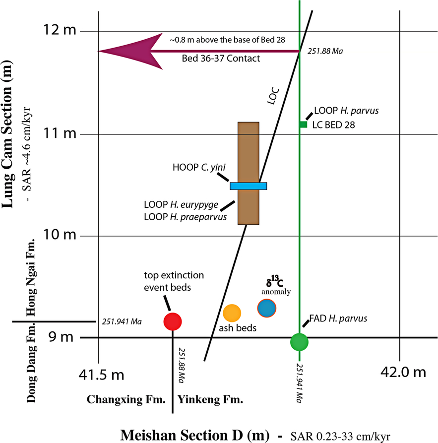
Herein it is shown that the expanded PTB succession at Lung Cam in Vietnam, which is well correlated to the Meishan D section PTB GSSP in China (Figs. 1, 2; Nestell et al. Reference Nestell, Nestell, Ellwood, Wardlaw, Basu, Ghosh, Lan, Rowe, Hunt, Tomkin and Ratcliffe2015; Wardlaw et al. Reference Wardlaw, Nestell, Nestell, Ellwood and Lan2015), can be effectively used to correlate to successions where the GSSP-defining fossils and related biostratigraphy is not well defined or missing. The Lung Pu section in Vietnam (Fig. 1) has been chosen for this comparison. The GSSP for the base of the Triassic at the Meishan D section is based on the FAD within the section of the conodont species Hindeodus parvus. This precise occurrence defines the position in time of the PTB. However, elsewhere, H. parvus may appear earlier or later, and therefore Wardlaw et al. (Reference Wardlaw, Nestell, Nestell, Ellwood and Lan2015) have argued that other than at the GSSP section, rather than the FAD, the LOOP should be used in identifying the stratigraphically lowest appearance of H. parvus. These authors used graphic correlation (Shaw, Reference Shaw1964) to compare the Meishan PTB section to the Lung Cam section in Vietnam (Fig. 3, modified from Wardlaw et al. Reference Wardlaw, Nestell, Nestell, Ellwood and Lan2015), and argued that the LOOP of H. parvus at Lung Cam is essentially coeval to the FAD at the GSSP. The results of this work (Nestell et al. Reference Nestell, Nestell, Ellwood, Wardlaw, Basu, Ghosh, Lan, Rowe, Hunt, Tomkin and Ratcliffe2015; Wardlaw et al. Reference Wardlaw, Nestell, Nestell, Ellwood and Lan2015) allowed the development of high-resolution timing for the Lung Cam section, using time-series analysis of magnetic susceptibility (χ) data for the PTB interval in the Lung Cam section, Vietnam. The problem with the Lung Pu test section is that no conodonts were recovered. Therefore, to correlate the Lung Pu section back to the GSSP, other stratigraphic methods are required.

Fig. 1. Location map of the Lung Cam (LC) and Lung Pu (LP) sections in a Permian limestone platform in northernmost Vietnam, relative to the Meishan GSSP in China.

Fig. 2. Stratigraphic column for the Lung Cam section correlated to the GSSP at Meishan D, China. The extinction event at Lung Cam refers to all extinctions through Lung Cam Beds 10 and 11 and does not represent a single point in time. These extinctions are represented in both sections. Note that the thickness from top of the extinction event at Meishan to the PTB is ∼0.38 m, whereas at Lung Cam, the thickness from the top of the extinction event to the PTB is ∼2.8 m.

Fig. 3. Graphic correlation diagram between the Lung Cam section, Vietnam, and the Meishan PTB GSSP section, China (modified from Ellwood et al. Reference Ellwood, Wardlaw, Nestell, Nesrell and Lan2017). The line of correlation (LOC) defines the Permian–Triassic boundary between Lung Cam Beds 36 and 37, and falls ∼0.8 m above the lowest observed occurrence point (LOOP) of Hindeodus parvus in Bed 28 in the Lung Cam section.
2. Methods
2.a. Magnetic susceptibility (χ)
All substances are ‘susceptible’ to becoming magnetized in the presence of an external magnetic field, and initial low-field bulk mass-specific magnetic susceptibility (χ) is an indicator of the strength of this transient magnetism. χ in marine stratigraphic successions is generally considered to be an indicator of detrital iron-containing paramagnetic and ferrimagnetic grains, mainly ferromagnesian and clay minerals (Bloemendal & de Menocal, Reference Bloemendal and de Menocal1989; Ellwood et al. Reference Ellwood, Crick, El Hassani, Benoist and Young2000, Reference Ellwood, Tomkin, Febo and Stuart2008; da Silva & Boulvain, Reference da Silva and Boulvain2002, Reference da Silva and Boulvain2005). It can be quickly and easily measured on small friable samples. In the very low inducing magnetic fields that are generally applied, χ is largely a function of the concentration and composition of the magnetizable material in a sample.
Low-field magnetic susceptibility, as used in most reported studies, is defined as the ratio of the induced moment (Mi or Ji) to the strength of an applied, very low-intensity magnetic field (Hj), where
 $${{\bf{J}}_{\bf{i}}} = {\chi _{ij}}{{\bf{H}}_{\bf{j}}}\ \left( {{\rm{mass - specific}}} \right).$$
(1)
$${{\bf{J}}_{\bf{i}}} = {\chi _{ij}}{{\bf{H}}_{\bf{j}}}\ \left( {{\rm{mass - specific}}} \right).$$
(1)
or
 $${{\bf{M}}_{\bf{i}}} = {k_{ij}}{{\bf{H}}_{\bf{j}}}.\left( {{\rm{volume - specific}}} \right).$$
(2)
$${{\bf{M}}_{\bf{i}}} = {k_{ij}}{{\bf{H}}_{\bf{j}}}.\left( {{\rm{volume - specific}}} \right).$$
(2)
In these expressions, the magnetic susceptibility in SI units is parameterized as κ, indicating that the measurement is relative to a one cubic metre volume (m3) and therefore is dimensionless; or magnetic susceptibility is parameterized as χ and indicates measurement relative to a mass of one kilogram, and is given in units of m3/kg.
2.b. Field sampling
In the field, the Lung Cam and Lung Pu sections were first cleaned using scrapers and brushes, so that all beds and lithologies were well exposed. Highly weathered zones were cleaned by digging, chipping and brushing, and these zones were noted in the field for evaluation of possible alteration effects. In both the Lung Cam and Lung Pu successions reported herein, samples were collected for χ and geochemical measurement at ∼0.05 m intervals, and for biostratigraphic analysis, bulk samples ( > 1 kg) were collected at ∼0.5 m intervals, and returned to the laboratory for study. Some of the results of the biostratigraphic analysis have been reported elsewhere (Nestell et al. Reference Nestell, Nestell, Ellwood, Wardlaw, Basu, Ghosh, Lan, Rowe, Hunt, Tomkin and Ratcliffe2015; Wardlaw et al. Reference Wardlaw, Nestell, Nestell, Ellwood and Lan2015). In addition, new geochemical data for the Lung Cam section are reported herein as well as correlated datasets from the Lung Pu succession that are not reported elsewhere.
2.c. Laboratory measurement of χ
The χ measurements reported in this paper were performed using the susceptibility bridge at Louisiana State University (LSU). The bridge is calibrated relative to mass using standard salts reported by Swartzendruber (Reference Swartzendruber1992) and CRC tables. For each group of measurements, each day laboratory standards were measured and compared to previous measurements to ensure that the bridge was performing properly. The χ data are reported in terms of sample mass because it is much easier and faster to measure with high precision than is volume, and it is now the standard for χ measurement. The low-field χ bridge at LSU can measure diamagnetic samples at least as low as −4 × 10⁻⁹ m3/kg. This precise measurement is illustrated by two relatively pure calcite samples from a standing speleothem collected from Carlsbad Caverns National Park (New Mexico, USA), where values are −3.37 × 10⁻⁹ and −3.46 × 10⁻⁹ m3/kg and standard deviations for three measurements are 7.64 × 10⁻¹¹ and 8.69 × 10⁻¹¹ m3/kg, respectively. These samples are used as standards for additional calibration when very weak samples are being measured. Note that in the Lung Cam section (Figs. 4, 5), a large proportion of the samples from the base of the section, up to ∼5.5 m, are diamagnetic (the diamagnetic field is noted in Figs. 4, 5). In the Lung Pu section for comparison, diamagnetic samples are found from the base to the ∼11 m point (Figs. 5–7), where there is a shift to paramagnetic values throughout the rest of the section. This shift appears to represent the onset of Siberian Traps volcanism as recorded in the Lung Cam and Lun Pu sections.

Fig. 4. Magnetic susceptibility (χ) with height in the Lung Cam section, Vietnam (∼21 m at a 0.05 m sample interval) showing χ and lithologic logs with key beds identified (a truncated version has been published by Nestell et al. Reference Nestell, Nestell, Ellwood, Wardlaw, Basu, Ghosh, Lan, Rowe, Hunt, Tomkin and Ratcliffe2015). The Black Carbon and extinction levels are from Nestell et al. (Reference Nestell, Nestell, Ellwood, Wardlaw, Basu, Ghosh, Lan, Rowe, Hunt, Tomkin and Ratcliffe2015). Ash beds, the graphically correlated Permian–Triassic boundary (PTB) and major Permian extinction levels are identified. The black/white bar-logs represent high (black) versus low (white) magnetic susceptibility (χ) values shown in the dashed curve connecting data points. Significant ash beds are labelled in the lithologic log. Onset of major Siberian Traps volcanism is placed at the point where mainly diamagnetic -χ values shift to only paramagnetic +χ values. Three isolated ash beds are identified below this level.
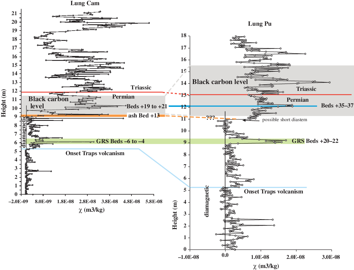
Fig. 5. Correlation of the well-defined Lung Cam section to the poorly defined Lung Pu section; ∼45 km separation between sections (Fig. 1). Correlation beds are: (1) the base of the Black Carbon layer; (2) a spike in χ values following a shift from diamagnetic χ values to much higher paramagnetic values in both sections, indicating the onset of Siberian Traps volcanism; (3) ash Bed + 13 in Lung Cam appears to coincide with the short diastem in Lung Pu; (4) gamma ray spectra (GRS) identified as relatively high in both sections.
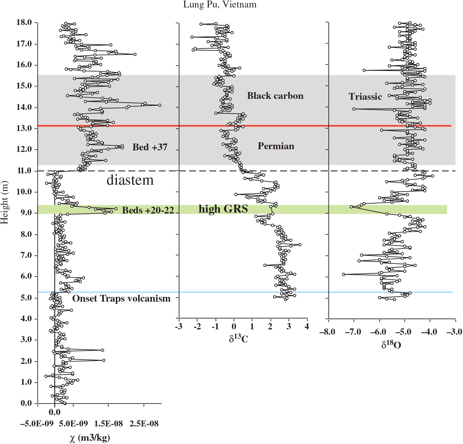
Fig. 6. Lung Pu χ data and stable isotope values for δ13C and δ18O. Also given are gamma ray spectra (GRS) levels and the Black Carbon interval in the section. A short diastem is inferred from the abrupt χ shift observed at ∼11 m in the section. Onset of Siberian Traps volcanism is identified.
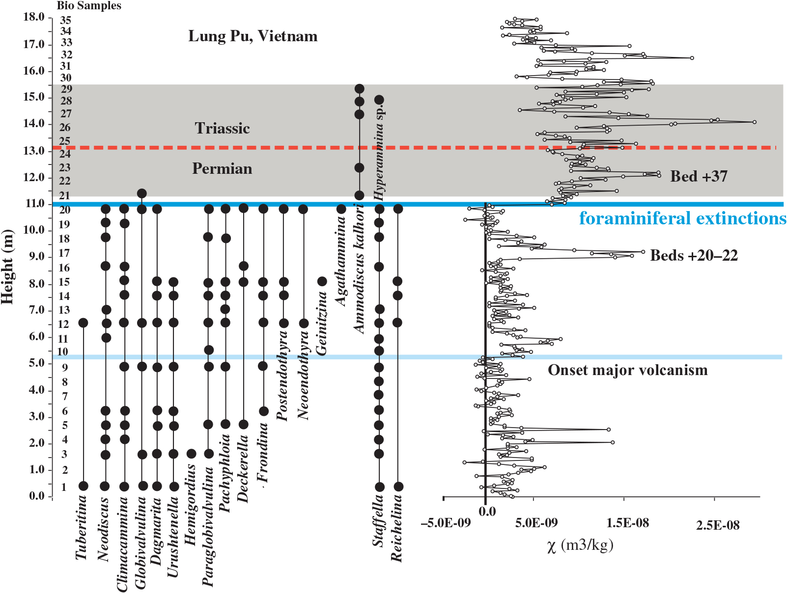
Fig. 7. Distribution of foraminiferal genera and species from biosamples collected from the Lung Pu sequence. Note that there is a major ‘extinction event’ in the foraminiferal dataset at ∼11 m in the section, also inferred from the χ data at that level indicating a diastem (erosion or non-deposition). Onset of Siberian Traps volcanism is identified.
2.d. Sample preparation and whole-rock geochemical analyses
Samples were collected from the expanded Lung Cam section to establish a geochemical database for the PTB at that site in Vietnam. Where possible, samples that showed no influence of superficial weathering were collected, and any weathering rinds were carefully removed prior to preparation. The samples were then ground to a powder in a ball mill and, following Li-metaborate fusion, analysed using inductively coupled plasma optical emission spectrometry (ICP-OES) and mass spectrometry (ICP-MS). The methods of fusion and analysis are those described in Jarvis & Jarvis (Reference Jarvis, Jarvis, Jarvis and Jarvis1995). These analytical methods result in data for 50 elements (10 major elements, reported as oxide per cent by weight: SiO2, TiO2, Al2O3, Fe2O3, MgO, MnO, CaO, Na2O, K2O and P2O5); 25 trace elements, reported as parts per million by weight (ppm) (Ba, Be, Bi, Co, Cr, Cs, Cu, Ga, Hf, Mo, Nb, Ni, Pb, Rb, Sn, Sr, Ta, Tl, Th, U, V, W, Y, Zn and Zr); and 14 rare earth elements (REE), reported as ppm (La, Ce, Pr, Nd, Sm, Eu, Gd, Tb, Ho, Dy, Er, Tm, Yb and Lu). Precision errors for the major-element data were generally better than 2 %, and around 3 % for the high-abundance trace-element data derived by ICP-OES (Ba, Cr, Sc, Sr, Zn and Zr). The remaining trace-element abundances were determined by ICP-MS, and data were generally less precise, with precision errors in the order of 5 % ± 1 % for major and ± 3 to 7 ppm for trace elements, depending on abundance. Expanded uncertainty values (95 % confidence), which incorporate all likely errors within a statistical framework derived from 11 batches of 5 certified reference materials, each prepared in duplicate, are typically 5–7 % (relative) for major elements and 7–12 % (relative) for trace elements.
Chemostratigraphy, as reported herein (Figs. 8–10), is the discipline of characterizing and subdividing sequences based on changes in their whole-rock inorganic geochemical composition. Most commonly, chemostratigraphy has been applied to provide correlations between relatively closely spaced sections for the petroleum industry (e.g. Pearce et al. Reference Pearce, Besly, Wray and Wright1999; Ratcliffe et al. Reference Ratcliffe, Wright, Hallsworth, Morton, Zaitlin, Potocki and Wray2004, Reference Ratcliffe, Wright, Montgomery, Palfrey, Vonk, Vermeulen and Barrett2010). The resultant chemostratigraphic correlations are based upon changes in chemistry that reflect subtle changes in mineralogy, which in turn reflect changes in sediment provenance (Ratcliffe et al. Reference Ratcliffe, Wright, Hallsworth, Morton, Zaitlin, Potocki and Wray2004, Reference Ratcliffe, Morton, Ritcey and Evenchick2008), changes in facies (Svendsen et al. Reference Svendsen, Henrik, Stollhofen and Hartley2007) or changes in palaeoclimate (Pearce et al. Reference Pearce, Wray, Ratcliffe, Wright, Moscariello, Collinson, Evans, Holliday and Jones2005). By enabling very subtle changes in such parameters to be modelled, the technique is capable of providing high-resolution correlations. In the case of modelling changes in detrital mineralogy, the correlation scheme produced is essentially lithostratigraphic, and therefore any stratigraphic correlation is likely to be of restricted extent (Ratcliffe et al. Reference Ratcliffe, Wilson, Payenberg, Rittersbacher, Hildred and Flint2015).
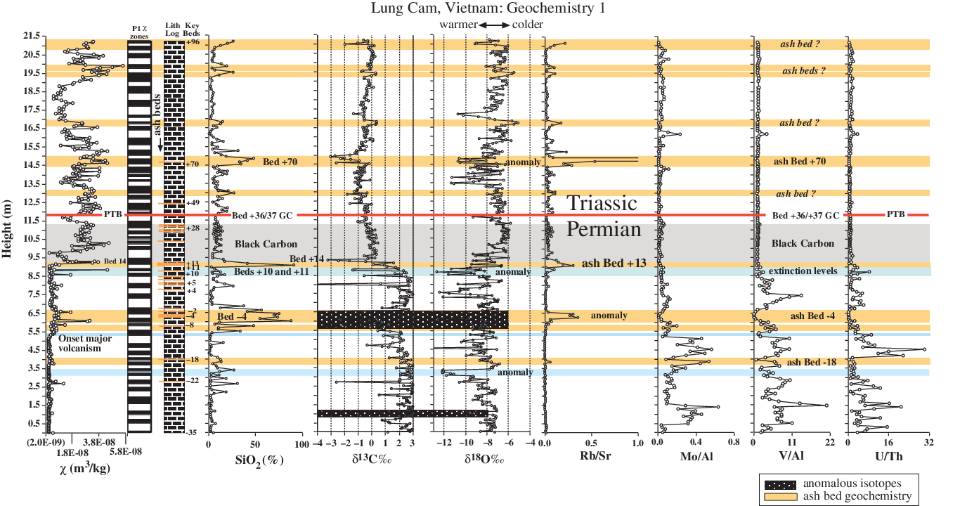
Fig. 8. The Lung Cam section, Vietnam, where χ, SiO2, δ13C, δ18O, and Rb/Sr, Mo/Al, V/Al and U/Th elemental ratios are plotted relative to depth in section. Layers coloured tan in the diagram are ash beds that are not climate related and therefore the stable isotopes behave differently from limestone samples. Added to the plot is a lithologic log with ash beds identified, key beds, the graphic correlation (GC) PTB at the contact between Beds + 36/ + 37 (solid red line), ash beds and the Black Carbon (grey shaded) level reported by Nestell et al. (Reference Nestell, Nestell, Ellwood, Wardlaw, Basu, Ghosh, Lan, Rowe, Hunt, Tomkin and Ratcliffe2015). Onset of Siberian Traps volcanism is identified.
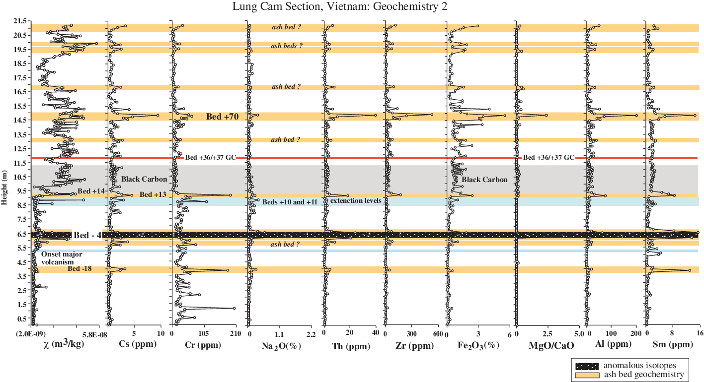
Fig. 9. The Lung Cam section where χ and geochemical data, Cs, Cr, Na2O, Th, Zr, Fe2O3, MgO/CaO, Al and Sm are plotted for comparison. Also identified are ash beds, a zone of anomalous stable isotope results, the Black Carbon horizon, the PTB and the extinction event Beds + 10 and + 11. Onset of Siberian Traps volcanism is identified. High Th values are associated with ash bed alteration to clays.
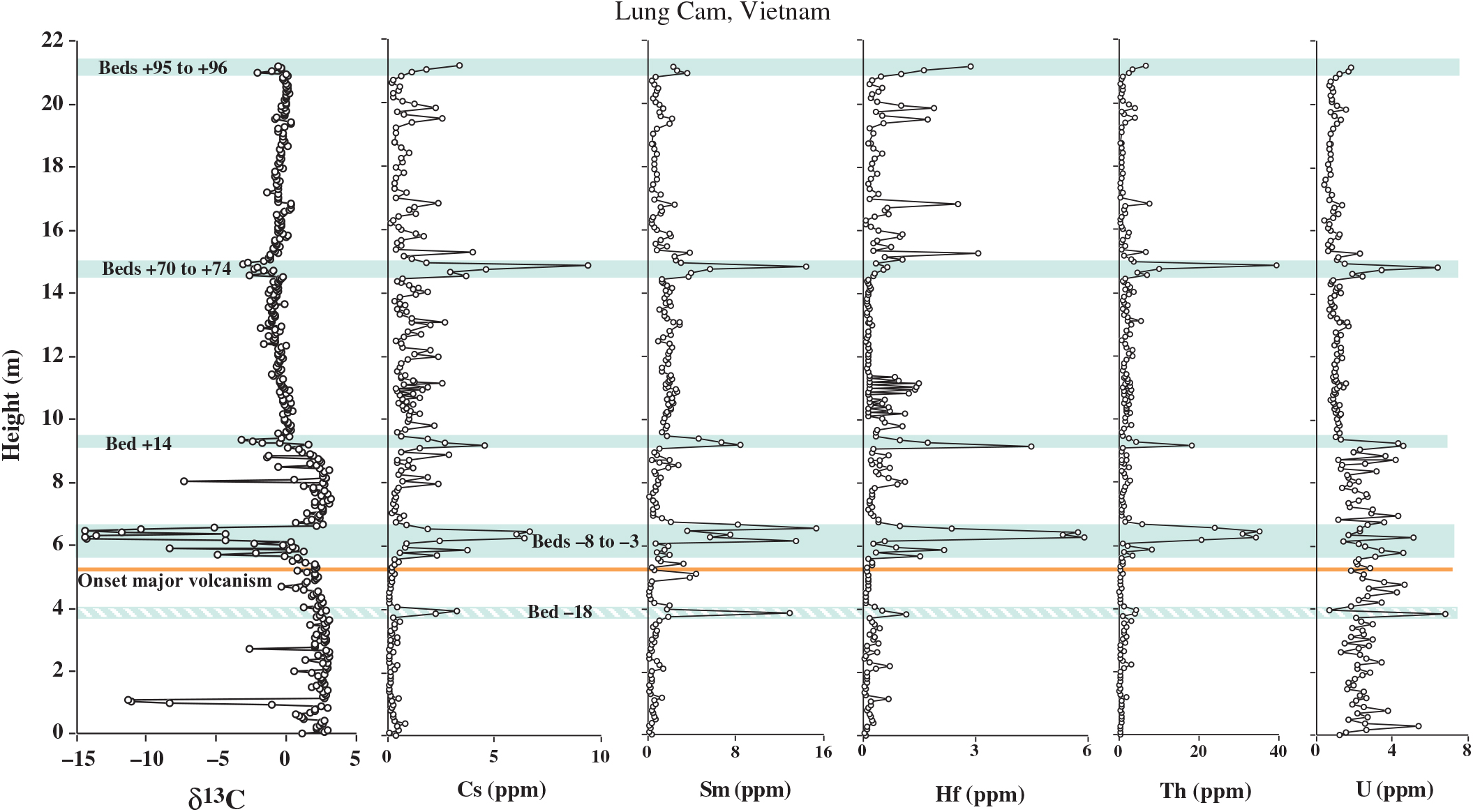
Fig. 10. Comparison of Lung Cam section geochemistry, Cs, Sm, Hf, Th and U, to anomalies in the δ13C data. Note that with the exception of geochemical anomalies in Bed −18, all anomalies shaded in light blue are also associated with a δ13C anomaly. However, the large δ13C anomaly in the base of the section, at the ∼1.0 m level, does not correlate to an anomaly in the geochemistry, but it does represent a zone of fault gauge indicating alteration at that level. Onset of Siberian Traps volcanism is identified.
2.e. Measurement of stable isotopes for δ 13C and δ 18O analyses of the Lung Cam and Lung Pu successions in Vietnam; samples also measured for χ
Approximately 0.325 mg of rock sample were loaded into Exetainer vials, capped and flushed with He reacted with phosphoric acid, and equilibrated for 13 hours at 50 °C. Stable carbon and oxygen isotopic compositions of the sample were analysed in continuous flow mode using a Thermo-Finnigan Gas-Bench II coupled to a Delta V isotope ratio mass spectrometer. Reproducibility (standard deviation) of the in-house standard, NBS-19, NBS-18 and the foraminiferal samples is 0.1 ‰ for both δ13C and δ18O. Isotopic values are reported with respect to the Vienna Pee Dee Belemnite (V-PDB) (Figs. 8–10).
2.f. Graphic correlation and graphic comparison
Graphic correlation (Shaw, Reference Shaw1964), primarily of the conodont zones observed in common to both the Meishan GSSP and the Lung Cam sections, was used to identify the PTB height within the Lung Cam section (Fig. 3, modified from Wardlaw et al. Reference Wardlaw, Nestell, Nestell, Ellwood and Lan2015). Added to the conodont data are the tops of the extinction event levels as well as a δ13C anomaly common to both sections, and the bases of GSSP Bed 25 (Meishan) and equivalent Bed +13 (Lung Cam) ash beds.
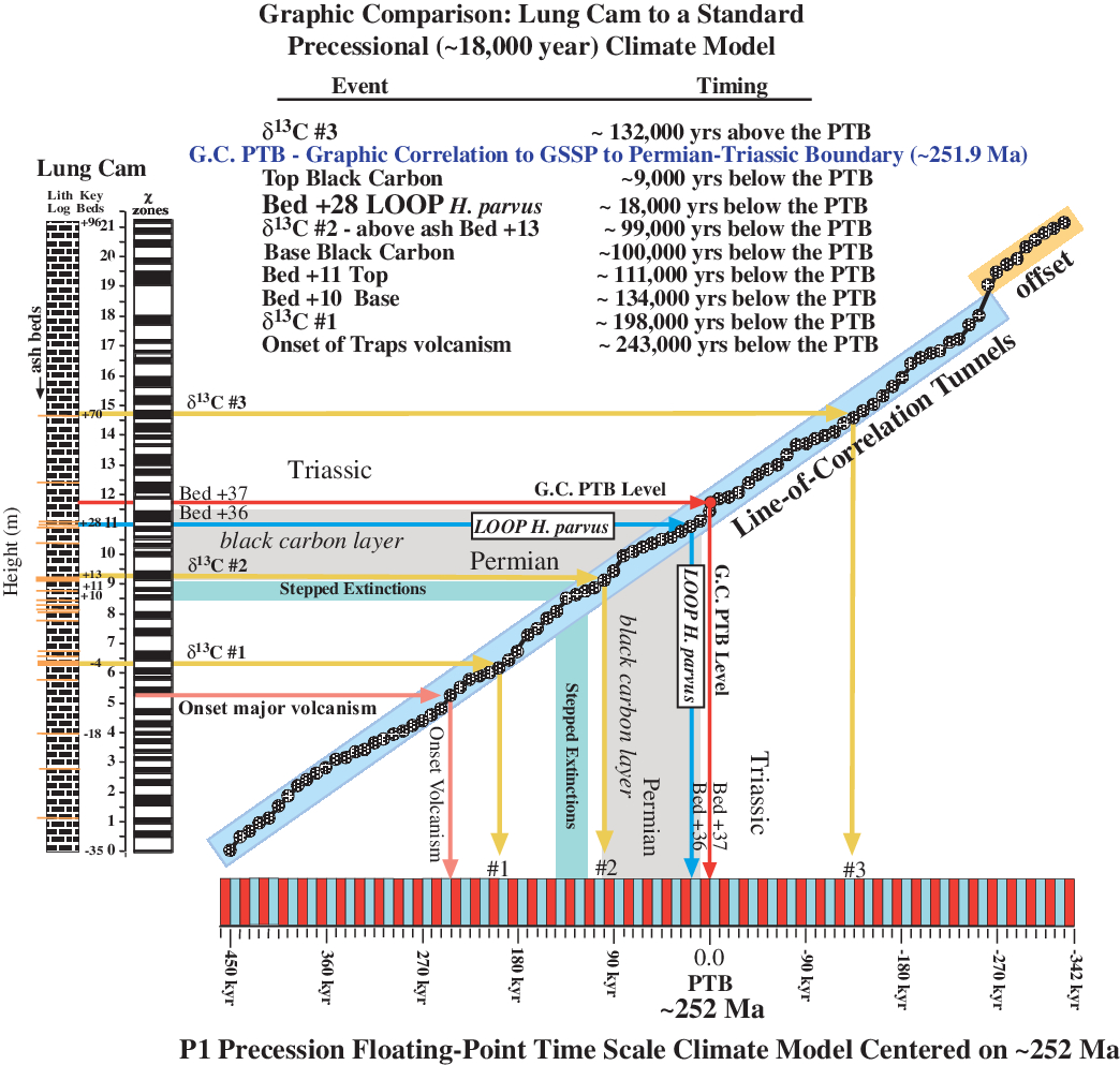
Graphic comparison was used in developing floating-point time scales for these data (Fig. 11). To do this comparison, first a uniform climate model for P1 (18 kyr precession) cyclicity was established and compared to the χ zones in Figure 4, where the uniform P1 model was graphically compared to the bottoms and tops of corresponding χ zones by plotting their intersections and drawing a line of correlation (LOC) through these intersections (Fig. 12). The process is roughly similar to graphic correlation. Lastly, a bounding tunnel enclosing these straight-line LOC segments was drawn to allow visual estimation of cyclic variability caused by other cyclic components in the data.

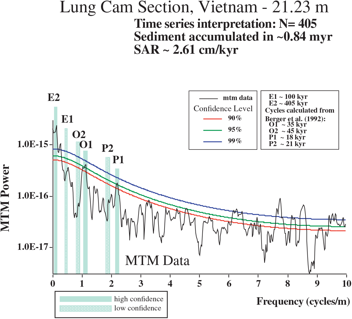
Fig. 11. Time-series analysis using the multi-taper method (MTM) for the 21.23 m Lung Cam section, using χ data for 405 samples, collected at 0.05 m intervals through the succession. The legend gives confidence levels and the Milankovitch bands identified in the dataset (modified from Lan et al. Reference Lan, Ellwood, Tomkin, Nestell, Nestell, Ratcliffe, Rowe, Huyen, Nguyen, Nguyen, Nguyen and Dao2018).

Fig. 12. Graphic comparison between the Lung Cam P1 data from time-series analysis of χ bar-log data and a P1 precession uniform time-scale model for the PTB interval (Nestell et al. Reference Nestell, Nestell, Ellwood, Wardlaw, Basu, Ghosh, Lan, Rowe, Hunt, Tomkin and Ratcliffe2015). The legend above the line of correlation (LOC) gives timing derived from this model as a result of projecting lithologies and geochemistry from the Lung Cam χ bar-log through the LOC tunnel and into the P1 time-scale climate model in Figure 11. Onset of Siberian Traps volcanism is identified.
3. Results
3.a. Magnetic susceptibility (χ) for the Lung Cam and Lung Pu sections, Vietnam
The χ data for the Lung Cam section are reported in Figure 4. Included in the diagram are the PTB, lying between Bed +36/ +37 (red line identified using graphic correlation by Nestell et al. Reference Nestell, Nestell, Ellwood, Wardlaw, Basu, Ghosh, Lan, Rowe, Hunt, Tomkin and Ratcliffe2015; modified very slightly herein, Fig. 3); the Black Carbon layer (i.e. wildfire and/or global fly ash) identified based on the presence of the agglutinated foraminifers Ammodiscus kalhori and Hyperammina sp., found in the Lung Cam section (Nestell et al. Reference Nestell, Nestell, Ellwood, Wardlaw, Basu, Ghosh, Lan, Rowe, Hunt, Tomkin and Ratcliffe2015) and in the Lung Pu section; four prominent ash beds (orange fill), the limestone Beds +10 and +11 containing the extinction events (blue green fill); the distinctive δ13C anomaly, also identified in the GSSP (Yin et al. Reference Yin, Zhang, Tong, Yang and Wu2001); the lithologic log, including the many ash beds in orange (some very thin ash beds were not sampled but only observed) with some key beds numbered; and the measured χ data (dots) connected by dashed lines. The paramagnetic and diamagnetic sample regions are also identified in Figure 4.
Both the Lung Cam and Lung Pu sections have distinctively similar χ datasets (Fig. 5), and are correlated herein on that basis. Correlation is supported by the identification of the base of the Black Carbon layer, a gamma ray spectra (GRS) anomaly in Beds −6 to −4 in the Lung Cam section and Beds 20–22 in the Lung Pu section, and from the χ data cyclicity through the interval at Lung Cam and Lung Pu from 6.0 m to 14.0 m in both sections. Note that there is a short diastem identified only in the Lung Pu section just below 11.0 m that is based on the missing Bed +13 ash bed in the Lung Pu section at ∼11.0 m, expected because it is identified at Lung Cam (orange solid and dashed lines in Fig. 5), and the anomalous abrupt offset of the χ data at that level.
3.b. Foraminifers from Lung Pu biosamples
In almost all PTB sections in the Palaeo-Tethys where foraminifers have been studied, their extinction appears to have been sometimes gradual and sometimes abrupt. In all of these sections, a rich Permian foraminiferal assemblage is replaced by a very poor post-extinction assemblage consisting mostly of opportunistic species such as Ammodiscus kalhori (Brönnimann, Zaninetti and Bozorgnia), Hyperammina (former Earlandia) deformis (Bérczi-Makk), and the rare holdover taxa Globivalvulina sp. and Geinitzina sp. (Angiolini et al. Reference Angiolini, Cheeconi, Gaetani and Rettori2010; Krainer & Vachard, Reference Krainer and Vachard2011; Nestell et al. Reference Nestell, Nestell, Ellwood, Wardlaw, Basu, Ghosh, Lan, Rowe, Hunt, Tomkin and Ratcliffe2015; Song et al. Reference Song, Tong, Wignall, Luo, Tian, Song, Huang and Chu2016; Kolar-Jurkovšek et al. Reference Kolar-Jurkovšek, Jurkovšek, Nestell and Aljinović2018; Sudar et al. Reference Sudar, Kolar-Jurkovsek, Nestell, Jovanovic, Jurkovsek, Williams, Brookfield and Stebbins2018). In the Lung Pu section, the extinction of most foraminiferal genera appears to be sudden, as can be seen in Figure 7. The last and relatively rich Permian foraminiferal generic assemblage is present in Biosample 20 (Fig. 7), whereas immediately above it (in Biosample 21), the opportunistic species A. kalhori appears, and the holdover taxon Globivalvulina sp. continues to be present. The species A. kalhori also occurs in biosamples 23, 27, 28 and 29, and the first Hyperammina sp. appears in Biosample 28. Such a sharp disappearance of genera of Permian foraminifers is considered to have been connected to a changing palaeoenvironment, resulting in different lithofacies or possibly an unconformity in the Lung Pu section, which is reflected in the χ data offset just above Biosample 20 in the section (Fig. 7).
3.c. Elemental geochemistry
Figures 8–10 show the χ values (Fig. 4) and stable isotope and geochemical data for the Lung Cam section. The extinction levels distributed through Beds +10 and +11 (Fig. 7; Nestell et al. Reference Nestell, Nestell, Ellwood, Wardlaw, Basu, Ghosh, Lan, Rowe, Hunt, Tomkin and Ratcliffe2015) are identified by light blue shading at ∼8.5 to 9.0 m height in the section. The main ash beds identified by unique geochemical variations that exhibit a similar signature to that in ash Bed +13 (equivalent to the Meishan D section Bed 25 and 26) are identified by light orange shading and given bed numbers where identified and sampled in the field (Bed −18, Bed −4, Bed +13, Bed +70). The chemical signature for these ash beds (bentonites) is used as a ‘fingerprint’, as observed in the Rb/Sr values in Figure 8 and Cs, Cr, Th, Zr, Al and Sm values in Figure 9, and in Figure 10 the ash bed signature in Cs, Sm, Hf, Th and U is also correlated with δ13C anomalies in the section. The chemical signatures in beds in the upper part of the section, labelled as ‘ash bed?’ (Figs. 8, 9), yield an ash bed geochemical signature, but no obvious ash bed was observed at that point in the outcrop during cleaning and sampling. Also plotted in Figures 8 and 9 are the PTB Black Carbon zone associated with elemental carbon incorporated within agglutinated foraminiferal tests (Nestell et al. Reference Nestell, Nestell, Ellwood, Wardlaw, Basu, Ghosh, Lan, Rowe, Hunt, Tomkin and Ratcliffe2015); ash bed or proposed ash bed levels; and δ13C and a distinctive δ18O shift observed in Figure 8. Aiding in characterizing and identifying ash beds in this dominantly marine sequence are SiO2 values in Figure 8. There are two anomalous δ13C and corresponding δ18O zones (stippled regions in Figs. 8, 9).
Mo/Al, V/Al and U/Th ratios are plotted in Figure 8 as indicators of anoxic (high values) versus oxic (low values) conditions during deposition of the sediments collected. The marine environment in the Lung Cam section, from the base of the section to the extinction levels, trends towards more anoxic conditions, whereas above the extinction levels the section appears to be relatively well oxygenated. Iron as Fe2O3 and MgO/CaO ratios are also given for the Lung Cam section in Figure 9.
3.d. Stable isotope geochemistry: δ 13C and δ 18O
δ13C and δ18O data are given for samples collected from the Lung Pu section (Fig. 6), and in Figure 8 for the Lung Cam section. The δ13C data show trends beginning at the base of both sections with values between 2 and 3 ‰, with some variability, including two large anomalous datasets at Lung Cam (stippled in Figs. 8, 9). Both of these zones show correlated δ13C and δ18O data variations and are clearly anomalous, and a similar pattern for Beds +20 to +22 in the Lung Pu section (Fig. 6) is also observed. An important δ13C peak in Lung Cam lies immediately above ash Bed +13 (equivalent to Bed 25 at Meishan) (Nestell et al. Reference Nestell, Nestell, Ellwood, Wardlaw, Basu, Ghosh, Lan, Rowe, Hunt, Tomkin and Ratcliffe2015), in Lung Cam Bed +14, and shows a negative ∼4 ‰ δ13C shift at the end of an overall gradual trend towards generally negative δ13C values that continue upwards through the PTB at Lung Cam (Fig. 8). However, in Lung Pu, this δ13C anomaly interval is missing because its correlation point falls within the proposed diastem (Figs. 5–7) and therefore appears to have been removed by erosion or resulted from non-deposition. As a result, whereas the overall stable isotopic variations are similar in both Lung Cam and Lung Pu, because of erosion at Lung Pu, the important Lung Cam Bed +14 δ13C anomaly is missing at Lung Pu.
In addition, there are interesting cycles exhibited in the Lung Cam δ18O dataset in limestone beds that we interpret to be associated with climatic variations. Therefore, in Figure 8, at the top of the δ18O column, a trend-arrow (excepting ash beds) is placed indicating warmer versus colder climate variations recorded in limestone beds in the section. An independent negative δ18O shift towards abrupt warming, of > 4 ‰, is identified by light blue shading between ∼3.0 and ∼3.5 m height in the Lung Cam section (Fig. 8).
3.e. Timing in the Lung Cam section
Figure 4 presents the entire measured section, expanded and supplemented from the work of Nestell et al. (Reference Nestell, Nestell, Ellwood, Wardlaw, Basu, Ghosh, Lan, Rowe, Hunt, Tomkin and Ratcliffe2015) and Lan et al. (Reference Lan, Ellwood, Tomkin, Nestell, Nestell, Ratcliffe, Rowe, Huyen, Nguyen, Nguyen, Nguyen and Dao2018) from ∼3.5 m to ∼21.2 m of section. Timing for the Lung Cam section is based on using time-series analysis (Fig. 11) and results essentially in the same timing as that reported using radiometric methods for the Meishan GSSP by Shen et al. (Reference Shen, Crowley, Wank, Bowring, Erwin, Henderson, Ramezani, Zhang, Shen, Wang, Wang, Mu, Li, Tang, Liu, Zeng, Jiang and Jin2011) and Chen et al. (Reference Chen, Shen, Li, Xu, Joachimski, Bowring, Erwin, Yuan, Chen, Zhang, Wang, Cao, Zheng and Mu2016).
3.f. Climate and the floating-point time scale
Isotopic studies of marine sediments/rocks rely on the assumption that isotopic (and cyclic lithologic) changes are a proxy for climatic cycles that are presumed to be global (i.e. Imbrie et al. Reference Imbrie, Hays, Martinson, Mc Intyre, Mix, Morley, Pisias, Prell, Shackleton, Berger, Imbrie, Hays, Kukla and Saltzman1984; Dinarès-Turell et al. Reference Dinarès-Turell, Baceta, Bernaola, Orue-Etxebarria and Pujalte2007). Tests of these hypotheses have shown that time-series data can provide a much higher resolution for time scales than are available using biostratigraphic information alone. Such datasets have not been documented for most of the Phanerozoic Eon, however, because stratigraphic sequences are imperfect recorders of time owing to erosion, non-deposition, bioturbation, alteration and other processes. As a consequence of these processes, short-term Milankovitch bands (Earth’s obliquity and precession) are not as well developed or easily recognized in older rocks as they are in younger sequences. However, it is now clear that time-series analysis of cyclic geophysical (i.e. χ and gamma ray spectroscopy; Ellwood et al. Reference Ellwood, Wang, Tomkin, Ratcliffe, El Hassani and Wright2013) and geochemical datasets are controlled by global processes often driven by climate cyclicity. It is now well established that χ datasets in both unlithified and lithified marine sediments can be used to track this cyclicity. Therefore, the cyclostratigraphy recorded in these sequences can be used for calibration of geologic time scales (Mead et al. Reference Mead, Tauxe and Labrecquel1986; Hartl et al. Reference Hartl, Tauxe and Herbert1995; Weedon et al. Reference Weedon, Shackleton, Pearson, Shackleton, Curry, Richter and Bralower1997, Reference Weedon, Jenkyns, Coe and Hesselbo1999; Shackleton et al. Reference Shackleton, Crowhurst, Weedon and Laskar1999; Crick et al. Reference Crick, Ellwood, El Hassani, Hladil, Hrouda and Chlupac2001). In addition to its utility in palaeoclimatic studies, magnetostratigraphic susceptibility (Salvador, Reference Salvador1994) can be used for high-resolution correlation among marine sedimentary rocks of broadly differing lithofacies with regional and global extent (Crick et al. Reference Crick, Ellwood, El Hassani, Feist and Hladil1997, Reference Crick, Ellwood, El Hassani and Feist2000; Ellwood et al. Reference Ellwood, Tomkin, Febo and Stuart2008; Whalen & Day, Reference Whalen, Day, Lukasik and Simo2008). The values of χ, when used as a correlation tool, provide a robust dataset to independently evaluate and adjust stratigraphic position among geological sequences. Reasonable biostratigraphic control is necessary to initially develop a chronostratigraphic framework where distinctive χ zones can be directly correlated with high precision among rock successions, even when biostratigraphic uncertainties or slight unconformities are known to exist within sections (Ellwood et al. Reference Ellwood, Garcia-Alcalde, El Hassani, Hladil, Soto, Truyóls-Massoni, Weddige and Koptikova2006, Reference Ellwood, Brett and Macdonald2007). The method is particularly useful for independent age control because it allows the extraction of data from sections that are not amenable to other magnetostratigraphic techniques, such as remanent polarity (Berggren et al. Reference Berggren, Kent, Aubry and Hardenbol1995; Gradstein et al. Reference Gradstein, Ogg, Schmitz and Ogg2012), as it does not require that the rock or sediment that is being analysed be oriented. The use of χ zones works as a climate proxy because regional and global processes that drive erosion, including climate and eustasy, bring detrital components responsible for the χ signature into the marine environment where its stratigraphy is preserved (Ellwood et al. Reference Ellwood, Crick, El Hassani, Benoist and Young2000).
Because χ zones have been shown to represent Milankovitch climate cyclicity, the χ data can also be considered as a floating-point time scale, with each χ zone representing a Milankovitch half cycle (Fig. 4). Then, depending on the absolute time scale used, it is possible to assign specific ages to each χ zone boundary and thus to estimate the timing of the biostratigraphic zonation used, bioevents identified in the sequence, overall time represented by the section and sediment accumulation rate.
To plug into a specific time scale, an absolute age must be used. If the time scale used is different or changes, it is a simple matter to recalculate the new age of the χ zone of interest. Timing of these zones can then be compared on a global scale to other sections using the χ zonation identified for those sequences, and high-resolution time-series ages can then be calculated.
The Lung Cam section in Vietnam is an expanded succession of ∼21 m of section through the PTB interval where ∼840 kyr of time is recorded (Fig. 11). Given that the Lung Cam section is well correlated to the GSSP section at Meishan (Nestell et al. Reference Nestell, Nestell, Ellwood, Wardlaw, Basu, Ghosh, Lan, Rowe, Hunt, Tomkin and Ratcliffe2015), it provides an excellent proxy to which other PTB sections, such as Lung Pu, can be compared. Herein, we use geophysical, geochemical and biostratigraphic information to correlate among two PTB successions, the Lung Cam section, Vietnam (Nestell et al. Reference Nestell, Nestell, Ellwood, Wardlaw, Basu, Ghosh, Lan, Rowe, Hunt, Tomkin and Ratcliffe2015; Wardlaw et al. Reference Wardlaw, Nestell, Nestell, Ellwood and Lan2015) and the GSSP Meishan D section (Fig. 2) in China (Yin et al. Reference Yin, Zhang, Tong, Yang and Wu2001). Each succession was deposited in the Palaeo-Tethys Ocean along the marine margins of the South China block, and the results presented herein provide unprecedented high-resolution timing, time-series dates and comparison to the GSSP using the Lung Cam succession.
The time-series results representing high-confidence P1 data (Fig. 11) were used to calculate overall timing in the Lung Cam section using graphic comparison to the Lung Cam χ data trends (Fig. 4). The well-defined LOC tunnel in Figure 12 indicates excellent consistency in the raw χ data trends when compared to a P1 incremental model. By projecting events identified in the Lung Cam dataset, through the LOC segment and into the P1 floating time-scale climate model (Fig. 12), it is possible to estimate the timing of these events. These events and corresponding times relative to the PTB are also given in Figure 4. These events (Fig. 12) include timing for three δ13C shifts: no. 1 at ∼198 kyr before the PTB; no. 2 at ∼99 kyr before the PTB; and no. 3 ∼132 kyr after the PTB. The stepped extinctions begin at ∼134 kyr (base of Bed +10) before the PTB, and then end at ∼111 kyr (top of Bed +11), indicating a duration of ∼27 kyr for these extinction events. The base of the Black Carbon layer in the Lung Cam section falls at ∼100 kyr before the PTB, whereas the top of the Black Carbon layer occurs at ∼9 kyr before the PTB, with a duration for the Black Carbon layer of ∼91 kyr (Fig. 12). This result may indicate that the duration of fires and global soot, presumably from Siberian Traps eruptions or unrelated synchronous volcanic eruptions in South China (Nestell et al. Reference Nestell, Nestell, Ellwood, Wardlaw, Basu, Ghosh, Lan, Rowe, Hunt, Tomkin and Ratcliffe2015), lasted for ∼91 kyr. The LOOP of H. parvus, at the base of Bed +28 in the Lung Cam section, occurs at ∼18 kyr below the PTB, and is graphically correlated to the Bed +36/ +37 bed boundary in the Lung Cam section. These data are slightly older (∼1000 years) than reported by Ellwood et al. (Reference Ellwood, Wardlaw, Nestell, Nesrell and Lan2017), and this new result is based on the higher resolution achieved in the new graphic correlation work reported herein (Figs. 3, 12).
4. Discussion
4.a. Lung Cam and Lung Pu sections, Vietnam
The Lung Cam and Lung Pu PTB successions were sampled at a uniform 0.05 m interval, and χ measurement for these samples shows two very distinctive trends in both successions (Figs. 4, 6) with (1) overall very low χ values, initially with χ < 1 × 10⁻⁸ m3/kg and many diamagnetic samples; and in Lung Cam ash Bed +13, equivalent to Beds 25 and 26 at Meishan, (2) there is a significant jump in χ that begins basically at Bed +17 where χ values climb to consistently higher levels (∼2 to ∼4 × 10⁻⁸ m3/kg) that show relatively well-defined cyclicity (Fig. 4). These values continue through the PTB at the top of Lung Cam Bed +36 (determined from graphic correlation in Fig. 3) to the top of the Lung Cam section, and these distinctive trends are similar to those reported for the Meishan GSSP in China (Hansen et al. Reference Hansen, Lojen, Toft, Dolenec, Tong, Michaelsen and Sarkar1999, Reference Hansen, Lojen, Toft, Dolenec, Tong, Michaelsen, Sarker, Yin, Dickins, Shi and Tong2000) and the Nhi Tao section, also in Vietnam (Algeo et al. Reference Algeo, Ellwood, Thoa, Rowe and Maynard2007).
At the Lung Pu section, there is a similar shift to much higher χ values, but this shift occurs at a hiatus in the section where Lung Cam Bed +13 should be exposed at Lung Pu, but instead appears to have been removed by erosion or non-deposition (diastem in Fig. 6). Above this level, the χ values increase significantly in correspondence with the shift in the Lung Cam section. These shifts to generally higher χ values are basically coeval with a shift to heavier δ18O values in Lung Cam (Fig. 8) and at Lung Pu (Fig. 6), suggesting a climate change in this region at that time to greater magnitude glacial–interglacial cyclicity and base-level changes, with corresponding erosion of terrestrial materials into the marine environment (discussed further in Section 4.c below). Higher rainfall may have also been an important factor.
4.b. Correlation and timing
The Lung Cam and Lung Pu sections in Vietnam are located in the South China block in shallower water than in the Meishan D GSSP section (Figs. 1, 2). Graphic correlation for both the Lung Cam and Meishan D successions shows that they are well correlated (Fig. 3). This result draws from conodont biostratigraphy in conjunction with unique correlated ash beds, extinction beds and δ13C anomalies. Using time-series analysis for the Lung Cam succession (Fig. 11) relative to the PTB level established herein (Fig. 4), it was possible to develop high-resolution ages for event horizons within the section. To do this, the high-confidence P1 (18 kyr precession) cycle was used, where the χ zones measured/calculated for the Lung Cam dataset were compared to a uniform P1 climate model (x-axis in Fig. 12). The following were then projected into the P1 floating-point time scale model for age identification relative to the PTB: (1) positions of the base of Bed +10 and top of Bed +11, encompassing the Late Permian ‘stepped’ extinctions; (2) the base and top of the Black Carbon level of Nestell et al. (Reference Nestell, Nestell, Ellwood, Wardlaw, Basu, Ghosh, Lan, Rowe, Hunt, Tomkin and Ratcliffe2015); (3) the PTB level determined using graphic correlation for the Lung Cam succession (Fig. 3); (4) the three main δ13C excursions in the Lung Cam section, and (5) the onset of Siberian Traps volcanism in these sections at ~242 kyr (Fig. 12; discussed below). This date is well within the uncertainties of Siberian Traps volcanism as dated by Burgess and Bowring (Reference Burgess and Bowring2015) at ~300+/−126 kyr below the PTB (Fig. 12; discussed below). The legend values then in Figure 12 represent plus or minus ages from ∼252 Ma (essentially the current value from the International Commission on Stratigraphy’s website (http://www.stratigraphy.org/GSSP/index.html).
The Black Carbon layer, representing carbon combustion due to fires burning or local volcanism at that time, is identified to represent ∼91 kyr of time through the PTB interval (Fig. 12). This elemental carbon was incorporated into the tests of two taxa of opportunistic benthic agglutinated foraminifers (Hyperammina deformis and Ammodiscus kalhori), and indicates the presence of carbon on the ocean floor at that time. The elemental carbon generated by global fires accumulated on the sea floor for a very long time, before and after the PTB (Nestell et al. Reference Nestell, Nestell, Ellwood, Wardlaw, Basu, Ghosh, Lan, Rowe, Hunt, Tomkin and Ratcliffe2015). However, the anoxic or perhaps dysoxic bottom water conditions that existed before the extinction events represented in Beds +10 and +11 at Lung Cam, and indicated by elemental ratios in Figure 8, would have precluded the appearance of these types of agglutinated foraminifers after the mass extinction event. The fact that they were living there at ∼100 kyr before the PTB indicates that favourable living conditions appeared for them at about this time (indicated by the beginning of the Black Carbon layer in Fig. 8), and therefore these types of opportunistic benthic foraminifers appeared after the extinction of calcareous foraminifers and were then able to survive. The same opportunistic species are found in other Palaeo-Tethys PTB successions, for example, in Slovenia, where black carbon has been found in agglutinated foraminifers associated with the boundary interval (Kolar-Jurkovšek et al. Reference Kolar-Jurkovšek, Jurkovšek, Aljinović and Nestell2011; Nestell et al. Reference Nestell, Kolar-Jurkovšek, Jurovšek and Aljinovic2011; Lan et al. Reference Lan, Ellwood, Tomkin, Nestell, Nestell, Ratcliffe, Rowe, Huyen, Nguyen, Nguyen, Nguyen and Dao2018).
The LOC tunnel developed from graphic comparison (Fig. 12) shows a well-developed dataset with some cyclic variability within the enclosing tunnel. These variations represent longer-term cycles superimposed upon the P1 dataset, with the main, long-term cyclicity representing high-confidence ∼405 kyr eccentricity cycles (Fig. 11).
4.c. Stable isotope geochemistry: δ 13C and δ 18O
Published δ13C studies for the Meishan GSSP section have shown a negative pulse in limestone Bed 27c of ∼−5 to −6 ‰ (Xu & Yan, Reference Xu and Yan1993), and a ∼−4 ‰ shift in ash Bed 25 (Jin et al. Reference Jin, Wang, Wang, Shang, Cao and Erwin2000 and others to a similar or lesser extent; e.g. Xie et al. Reference Xie, Pancost, Huang, Wignall, Yu, Tang, Chen, Huang and Lai2007; Chen et al. Reference Chen, Shen, Li, Xu, Joachimski, Bowring, Erwin, Yuan, Chen, Zhang, Wang, Cao, Zheng and Mu2016). In contrast, values at Lung Cam for both δ13C and δ18O vary depending on whether or not the measured sample comes from an ash bed or from a limestone. Ash bed samples, with a few exceptions, trend towards negative shifts in δ13C, and positive shifts in δ18O. Trends in limestone samples are discussed below. In two cases, there is clear alteration in samples interpreted to be ash beds/faulted surfaces. These are samples from 1 m (Bed −31 interpreted as fault gouge) and 5.5 to 6.5 m (fault gouge centred on Bed −4) in the Lung Cam measured section, and the isotopic results from these two levels do not apply in the following discussion.
Trends in δ13C at Lung Cam below the PTB show relatively consistent variations in limestone samples starting from +2 to +3 ‰ at the base of the measured section, followed by a general, slow negative shift through the extinction levels in limestone Beds +10 and +11, with some rapid and distinctive negative shifts of ∼−3 ‰, to just above ash Bed +13 (equivalent to Beds 25 and 26 at Meishan) in Lung Cam limestone Bed +14, where a well-defined abrupt negative shift of −3 to −4 ‰ occurs. These values then drop and stabilize in Bed +15 and range from −1 to 0 ‰, with a stable trend that continues up to and through the PTB. Above the PTB the character of the δ13C trend is a very slight trend towards values around ∼−1 ‰ until just above Bed +70, where values reach −3 ‰ and then fall just above Bed +72 to remain between −1 and 0 ‰, more or less through the rest of the section.
At Lung Pu, δ13C values above the diastem (Fig. 6) are similar to those trends at Lung Cam. These excellent and systematic trends, which are only slightly different from the GSSP (Fig. 3), can be explained by the higher resolution, larger dataset measured for the 90 % expanded Lung Cam section over the GSSP section at Meishan (Fig. 2).
From the base of the Lung Cam section upwards, δ18O values tend to be lighter, with a distinctive change just above Bed +13 (Fig. 8). At this level there is a trend in the δ18O results showing a general shift towards heavier isotopic values, a shift in δ18O values from −12 ‰ in Beds +10 and +11, the extinction levels, to −6 ‰ at the PTB. This +6 ‰ change, which appears to show a change towards a colder climate and glacial cyclicity through the interval containing black carbon within agglutinated foraminifers (Nestell et al. Reference Nestell, Nestell, Ellwood, Wardlaw, Basu, Ghosh, Lan, Rowe, Hunt, Tomkin and Ratcliffe2015), is also reflected in a shift in χ (Fig. 4). If colder, then this change is probably associated with enhanced glaciation at that time, thus increasing erosion that is reflected in increased χ values and the influx of more terrestrial components, e.g. higher iron (Fig. 9), into the marine environment. In addition, a change in the Mo/Al, V/Al and U/Th ratios observed in Figure 8 indicates a corresponding change from anoxic/dysoxic towards more oxic conditions above Bed +13, resulting from increased ocean circulation and mixing at that time. There are similar trends in δ18O values for samples from Lung Pu (Fig. 6) and Lung Cam (Fig. 8), above the Bed +20–22 GRS anomaly in Lung Pu, thus showing consistency between these two datasets in the region (Fig. 1).
4.d. Elemental geochemistry: ash bed signatures
Ash beds in the Lung Cam section exhibit some distinctive patterns, shown by the elemental geochemical data presented in Figures 9 and 10, which are supported by the Rb/Sr ratios reported in Figure 8. Identified ash beds, like Bed +13 (equivalent to Beds 25 and 26 at Meishan), show SiO2 peaks as well as high concentrations of Cs, Cr, Th, Zr, Al, Sm, Na (as Na2O) and Fe (as Fe2O3). These ash beds provide good tracers of volcanic ejecta. High elemental values at stratigraphic levels where no ash beds are observed in the section indicate the presence of ash in those samples, even though those ash layers were not identified in outcrop. These missed horizons are labelled as ‘ash bed?’ in Figures 8 and 9, and suggest that many more volcanic eruptions are recorded through the ∼840 kyr deposition of the Lung Cam succession than were obvious in outcrop. These data argue that, as for the modern Earth, where low-latitude dust from the Sahara Desert is distributed across the Atlantic Ocean and from Asia widely across the Pacific Ocean (Balsam et al. Reference Balsam, Otto-Bliesner and Deaton1995, Reference Balsam, Arimoto, Ji and Shen2007), so during PTB time, volcanic dust (ash) was deposited throughout the Palaeo-Tethys Ocean area, and this ash provides marker horizons that contribute to datasets used for high-resolution correlation and timing (Lan et al. Reference Lan, Ellwood, Tomkin, Nestell, Nestell, Ratcliffe, Rowe, Huyen, Nguyen, Nguyen, Nguyen and Dao2018).
Within the Lung Cam section, χ is mainly diamagnetic up to ∼5.5 m in the section (Fig. 4), with the last diamagnetic samples collected from Bed −12. In this zone of diamagnetic values, there are a few restricted zones where χ shows low paramagnetic values, and these are identified in outcrop as having a friable character typical of ash dispersed within thin limestone beds. Bed −22 (Fig. 4) is a good example of these characteristics. Given the ash bed levels identified, the onset of some volcanism at Lung Cam appears to have started associated with Bed −31 near the base of the section. Volcanism then ranges up through the succession to the top in Bed +96. This volcanism interval represents ∼800 kyr of time (Bed −31 to Bed +96), as calculated from the graphic comparison in Figure 12.
The geochemical signatures indicate that those ash beds in the upper part of the Lung Cam section, above the PTB, are mainly acidic, whereas the ash beds below the PTB are more mafic. This contrast is interesting when the Mo/Al, V/Al and U/Th ratios are compared, indicating more dysoxic or anoxic conditions below the PTB and oxic above the boundary. Did this chemical difference in these abundant ash beds perhaps cause or contribute to the anoxic/dysoxic conditions observed below the PTB, and thus contribute to the major extinctions in Beds +10 and +11? Our answer to this question is yes.
5. Conclusions
Herein, the PTB successions at Lung Cam and Lung Pu, Vietnam, have been tightly correlated to the Meishan D PTB GSSP section in China, where the FAD of H. parvus defines the PTB. Using graphic correlation of conodont species, extinction beds and known PTB geochemical and lithological signatures in Lung Cam, the data support the interpretation that the PTB from the Meishan D section can be projected into the Lung Cam Bed +36/ +37 contact. This PTB level lies ∼0.8 m above the LOOP of H. parvus, located at the base of Lung Cam Bed +28. Graphic correlation also shows that the well-correlated Lung Cam section is 90 % expanded relative to the Meishan PTB GSSP section (Figs. 2, 3), and therefore Lung Cam provides an extended sequence to which other PTB successions such as the Lung Pu succession can be correlated. This comparison is especially useful when conodont data are poor or missing in a PTB succession, as is the case at Lung Pu.
Time-series analysis of raw magnetic susceptibility (χ) data shows high significance in the E2 (∼405 kyr eccentricity; Fig. 11) and P1 (precessional) cyclic signals. Therefore, for the purpose of high-resolution dating, a uniform P1 climate model from Lung Cam, with cycles representing ∼18 kyr during PTB time, is used to establish a time scale for the PTB interval sampled in Vietnam. Comparison of the χ zones from Lung Cam to the P1 model allows detailed dating of beds/events represented in the section. Using this model (Fig. 12), it is shown that: (1) H. parvus arrived at Lung Cam ∼18 kyr before the date for the PTB FAD at the Meishan D section; (2) the black carbon generated by PTB fires and local volcanism, and incorporated within agglutinated benthic foraminiferal tests, first appears at Lung Cam ∼100 kyr before the PTB and lasts at Lung Cam until ∼9 kyr before the PTB; however, at Lung Pu, the black carbon was still present above the PTB to a correlated level in Lung Cam equivalent to the no. 3 δ13C anomaly at Lung Cam, approximately to Bed +70 level, indicating that these fires generated the elemental carbon found in the marine environment for at least ∼250 kyr; (3) three major δ13C anomalies are identified in the Lung Cam PTB succession: δ13C anomaly no. 1 occurred ∼200 kyr before the PTB, no. 2 occurred ∼100 kyr before the PTB and no. 3 occurred ∼130 kyr after the PTB; (4) δ18O data indicate a shift towards heavier values and thus colder climates starting just above Lung Cam Bed +13, at ∼ 100 kyr below the PTB, and continued above the ash Bed +70 level, a shift lasting for ∼250 kyr. These changes are interpreted from the cyclicity represented in the χ data that may have resulted in glacial–interglacial cycles and the enhanced erosional effects that lasted for hundreds of thousands of years. Finally, (5) the shift in χ from diagmagnetic (-χ) to paramagnetic (+χ) values at ~242 kyr before the PTB indicates the time of the beginnings of significant Siberian Traps volcanism.
Author ORCIDs
Brooks Ellwood, 0000-0003-2529-9734
Acknowledgements
This work was partly supported by the National Science Foundation [grant number EAR-0745393 to BBE], by the Vietnamese Academy for Science and Technology, and by the Robey Clark endowment to LSU. We thank Sue Ellwood for designing the sample method used and her aid in sampling, and Amber Ellwood for sample preparation and magnetic susceptibility measurements.