


1. Introduction
Benjamin's (Reference Benjamin1968) theory for the steady-state propagation of an inertial gravity current (GC) of density  $\rho _{c}$ into a homogeneous ambient is a widely accepted methodology for the study of buoyancy-driven currents and intrusions. The underlying idea is that the upstream and downstream flows are horizontal with hydrostatic pressure. For a control volume (CV) attached to the nose of the GC, the fundamental steady-state balances can be expressed by integrals over the simple flow on the boundaries of the CV, without the need for the details of the internal flow. The major result is a correlation of the speed of propagation,
  $U$, to
  $(g' h)^{{1/2}}$, where
  $h$ is the height of the current and
  $g'$ is the reduced gravity. The ratio
  $U/(g' h)^{{1/2}}$ is a ‘Froude number’ function of
  $a$, the height ratio of the current to the ambient. The homogeneous-ambient results are summarized in Appendix A.
Formally, the extension of this methodology to a system with a stratified ambient is possible. Such extensions, for Boussinesq systems, have been presented by Ungarish (Reference Ungarish2006) for a linearly stratified ambient and by White & Helfrich (Reference White and Helfrich2008) for a general stratification. The importance of stratification is measured by  $S = (\rho _b-\rho _{o})/(\rho _{c}-\rho _{o}) \in (0,1]$, where
  $b$ and
  $o$ indicate the bottom and top of the ambient. The connection between the upstream and downstream sides of the ambient is adapted from Long's solution for the stratified flow over a topography, and the obstacle is replaced by the GC. For weak stratification
  $S \ll 1$, the change from Benjamin's GC results is small, and for moderate
  $S$ (up to roughly 0.9) no special difficulties show up. As
  $S$ approaches
  $1$ (intrusion), the analysis discerns some qualitative novelties, such as restrictive instabilities and questionable patterns of energy dissipation of the possible fields that satisfy the balances. These intriguing issues are still inconclusive, perhaps because of lack of accurate experimental and simulation data.
The prototype geometry for the GC is a long horizontal channel of height  $H$ filled with stationary ambient fluid of density with linear decreasing stratification from
  $\rho _b$ to
  $\rho _{o}$, as sketched in figure 1. Into this fluid, at the bottom of the channel, a layer (current) of denser fluid of density
  $\rho _{c}$ and thickness
  $h$ propagates with uniform velocity
  $U$. The driving force is the reduced gravity,
 \begin{equation} g' = \epsilon g, \quad \text{where} \ \epsilon = \frac{\rho_{c} - \rho_{o}}{\rho_{o}}. \end{equation}
Another important dimensionless parameter is the fractional depth,
 \begin{equation} a=h/H. \end{equation}
The relative magnitude of the stratification is expressed by
 \begin{equation} S = \frac{\rho_{b}-\rho_{o}}{\rho_{c}-\rho_{o}}, \end{equation}
with  $0 < S \leqslant 1$. We assume a Boussinesq (
 $\epsilon \ll 1$), almost inviscid (Reynolds number
  $Re = U h /\nu \gg 1$) and shallow system in the sense that the typical horizontal length is large compared with
  $h$. Here
  $\nu$ is the kinematic viscosity of the fluids.

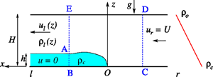
Figure 1. Sketch of the configuration. Here  $r$ and
  $l$ denote the upstream (right) and the downstream (left) positions; and BCDE is the control volume. For Long's solution, we define the lower boundary of the ambient as
  $z = \chi (x)$, and assume it is a solid free-slip obstacle. In general,
  $\rho _b <\rho _c$, and for the intrusion
  $\rho _b = \rho _c$.
The natural scaling speed is  $(g' h)^{{1/2}}$. The pertinent scaled speed of propagation, referred to as the Froude number of the GC, is
 \begin{equation} \hat{U} = Fr = \frac{U}{(g' h)^{{1/2}}}. \end{equation}
Now  $Fr$ is a function of both
  $a$ and
  $S$. We expect that the classical case (Benjamin's result) is recovered in the limit of a very mild stratification,
  $S\rightarrow 0$.
For further reference, we define the buoyancy frequency
 \begin{equation} \mathcal{N} = [(\rho_{b}/\rho_{o} - 1)g/H]^{{1/2}} = (Sg'/H)^{{1/2}}. \end{equation}
We recall that the speed of the fastest internal wave in the channel of height  $H$ is
 \begin{equation} V = \mathcal{N} H /{\rm \pi}, \end{equation}
and we keep in mind that higher modes, in particular with speed  $2 V$, may appear in the channel of
  $2 H$ symmetric about
  $z =0$.
The symmetric intrusion is conveniently analysed as a superposition of two GCs of the type sketched in figure 1. The plane  $z=0$ is the free-slip ‘bottom’ or ‘base’ boundary of the present model; the lower part is symmetric with respect to this plane. The geometry is a long current of height
  $h$ in a horizontal channel of height
  $H$, with given
  $a = h/H$. The scaling speed for the GC,
  $(g' h)^{{1/2}}$, is adopted in this paper also for the subsequent analysis of the intrusion. Suppose that a steady-state propagation of the intrusion with constant speed
  $U$ exists. In the spirit of Benjamin's analysis, this corresponds to a well-defined ‘Froude number’
  $Fr(a)$ (for
  $S=1$, to be distinguished from the classical
  $Fr(a)$ for
  $S=0$.)
The steady-state GC of Benjamin is an idealization. The following two are closely related realistic systems. (a) A GC released from a lock in a rectangular geometry displays, for a while (called the slumping stage), a nose that propagates with a constant speed followed by a current of constant height of quasi-steady behaviour (in a frame attached to the nose). (b) A GC sustained by a constant source also displays a nose of constant speed followed by a parallel flow. One can argue that such similarities between the idealization and realistic flows carry over to the intrusion in the linear stratification, but uncertainties appear because stratified systems are prone to contamination by internal-stratification waves.
The practical use of Benjamin's analysis result  $Fr_B(a)$ is in the derivation of a boundary condition for the nose jump of thin-layer (shallow-water) models for general GCs. The justification is as follows. The jump is a
  $\Delta x$ thin domain of fluid. The balances for a CV about the jump do not contain time-dependent terms because the volume and inertia of the embedded fluid are negligibly small. Consequently, the results of a steady current subjected to balances in the CV about the head (see figure 1) are also a solution of the nose jump instantaneous balances, although the jump is time-dependent. The steady-state solution is a rigorous problem, while the jump is an asymptotic approximation for
  $\Delta x /h \to 0$, and hence the correlation between the height and speed of the nose jump of a general GC can be approximated by an
  $Fr_B(a)$-type formula. The connection between the two problems still displays some uncertainties, because the rigorous steady-state solution needs some closures and is reliant on free-slip conditions and a sharp interface, which may be unattainable in practical flows; this produces some semi-empirical modification of
  $Fr_B(a)$, like the Huppert–Simpson formula (Huppert & Simpson Reference Huppert and Simpson1980).
In this context, we note that Ungarish & Huppert (Reference Ungarish and Huppert2002) derived a conjecture for the extension of the nose condition of a GC from a homogeneous  $S=0$ to a stratified
  ${S>0}$ case. The argument is that, in a system attached to the front,
  $Fr^{2}$ expresses the ratio of the dynamic pressure to the hydrostatic pressure at the base
  $z=0$; for a Boussinesq system, this ratio is dominated by the geometry,
  $a = h/H$ (not by the stratification). Assuming that the front of the current is a jump of height
  $h$, that the stratification of the ambient is not changed by the jump, and that there is pressure continuity at
  $z=h$, the result is
 \begin{equation} Fr(a,S) = Fr(a,S=0) \times [ 1 - S (1 - \tfrac{1}{2} a ) ] ^{{1/2}}. \end{equation}
Ungarish & Huppert (Reference Ungarish and Huppert2002) and Ungarish (Reference Ungarish2005) used this correlation for the nose condition in shallow-water models for GCs and intrusions (taking the semi-empirical Huppert–Simpson  $Fr(a,S=0)$ formula). They report good agreement of
  $U$ in various comparisons with laboratory and simulation data. Good agreement with simulations has also been reported by White & Helfrich (Reference White and Helfrich2008). However, we must keep in mind that these tests refer to the performance of the shallow-water model with stratification, not to the accuracy of the
  $Fr$ formula.
The present study is for  $S=1$. For consistency with the theoretical framework of this paper, we take
  $Fr(a,S=0) = Fr_B(a)$ provided by Benjamin's classical formula (Appendix A). Therefore, hereafter we express the correlation (1.7) as
 \begin{equation} Fr = U/(g' h)^{{1/2}} = Fr_B(a) \sqrt{a} /\sqrt{2}. \end{equation}
This we call the UH conjecture. Since this  $Fr$ lacks a rigorous CV derivation, it is difficult to subject it to insightful validity tests as used for the other results discussed below. We shall use it only for comparisons of numerical values.
The objective of the present work is to revisit this topic: the derivation of  $Fr$ for a symmetric intrusion in a linearly stratified ambient by Benjamin's steady-state method, and to elucidate the differences from the
  $Fr$ results for a homogeneous ambient. The organization of the paper is as follows. In § 2 we formulate the flow field and derive the governing balance and validity equations. In § 3 we present and analyse the results, in particular concerning the values of
  $Fr$ and dissipation. Comparisons with previously published direct numerical simulation (DNS) results (unfortunately, we found only one relevant point) and with the previously suggested
  $Fr$ conjecture formula are also discussed. In § 4 some concluding remarks are given. The classical homogeneous-ambient case and some comments on the head loss effect are summarized in Appendices A and B, respectively.
2. Formulation
2.1. The steady-state flow pattern
Following Ungarish (Reference Ungarish2006), we start with the solution of a two-dimensional stratified steady flow field over a rigid free-slip bottom topography (that mimics the dense fluid) in a channel with an upper free-slip horizontal lid at  $z=H$; see figure 1. The
  $\{x,z\}$ system is a frame of reference attached to the GC, the origin
  $O$ is the front stagnation point, the velocity components are
  $\{u,w\}$ and gravity acts in the
  $-z$ direction. We use dimensional variables unless stated otherwise. The idea is to explore the similarity between the flow configuration of a GC with an available result called Long's model (Long Reference Long1953, Reference Long1955) concerning the flow of a stratified fluid in a channel with an upper horizontal solid top and a prescribed bottom topography. As in the non-stratified case, the far-upstream velocity of the ambient is constant over the height of the channel,
  $0 \leqslant z \leqslant H$. This flow climbs the topography (current) at a relatively slow pace (compared with the horizontal propagation). The streamlines become horizontal again in the far-downstream region of the thinner channel,
  $h \leqslant z \leqslant H$. For an observer moving with the current (the bottom topography), the flow is steady.
In the non-stratified case, the downstream flow of the ambient fluid regains a uniform velocity,  $UH/(H-h)$, and a pressure field that is linear with
  $z$. This facilitates the calculations and simplifies the results. However, when
  $S>0$, the linear density stratification in the upstream region must be compressed in a non-trivial manner into a thinner channel. The downstream flow field of the ambient fluid develops a quite complex
  $z$-dependent structure of velocity, density and pressure. The first task is to specify this flow field.
The geometry is like that of figure 1, but the coloured domain is a part of the solid bottom (the obstacle). To be specific, the obstacle (or topography) encountered by the unperturbed stratified fluid is defined by the bottom elevation function,  $z=\chi (x)$. The value of
  $\chi$ is
  $0$ (i.e. no obstacle) for non-positive
  $x$. For
  $x>0$, the bottom is elevated to
  $\chi (x) >0$; and far downstream at the left, a parallel geometry is achieved again with
  $\chi (x) = h = \text {const.}>0$.
The far-upstream flow (at the right,  $x \rightarrow - \infty$), where the bottom is flat,
  $z=\chi (x) = 0$, consists of parallel horizontal streamlines with constant velocity
  $U$ and a prescribed stable linearly changing density. Using the subscript
  $r$ (right) to denote this region, we write
 \begin{equation} u_r(z) = U, \quad w_r(z) = 0, \quad \rho_{r}(z) = \rho_b - \widetilde{\Delta\rho} \times (z/ H), \end{equation}
where  $\widetilde {\Delta \rho } = \rho _b - \rho _{o} = S(\rho _c - \rho _{o})$ in general, and
  $\widetilde {\Delta \rho } = \rho _c - \rho _{o}$ for the intrusion (
 $S=1$) case that is the topic of this paper.
Under the assumption of a two-dimensional steady Boussinesq inviscid flow, the analysis of Long (Reference Long1953) can be applied to reduce the set of governing Euler equations to a single partial differential equation (PDE) for the displacement of the streamline,  $\delta (x,z)$, subject to the obvious
  $\delta = 0$ in the upstream right region, and
  $\delta =\chi (x)$ at the bottom. In the steady flow, streamlines and pathlines coincide, and hence the initial (upstream) density is conserved along these lines and allows the application of clear-cut conditions to the downstream domain for the flow over a simple bottom topography. Variants of the derivation method can be found in the literature; e.g. Shapiro (Reference Shapiro1992) includes the density variation by an Exner function, while Shivamoggi & Rollins (Reference Shivamoggi and Rollins2004) use a streamfunction for the modified velocity components
  $(\rho (z)/\rho _{o})^{{1/2}}\{u,w\}$. Mathematical manipulations produce a PDE for
  $\delta (x,z)$ (or the closely related streamfunction
  $\psi$), which, for some simple (but physically relevant) upstream conditions is a linear Helmholtz equation amenable to analytical solution. Here we use the analytical solution for the present configuration as reported in Baines (Reference Baines1995, chap. 5). The flow field is conveniently expressed with the aid of the perturbation (about the upstream flow) streamfunction,
  $-\partial \psi /\partial z =u'$,
  $\partial \psi /\partial x = w$, where
  $u=U+u'$. The result reads
 $$\begin{gather} \psi(x,z)=U \times \chi(x) \, \frac{\sin[\beta(1-z/H)]} {\sin[\beta(1-\chi(x)/H)]} = U \times \delta (x,z), \end{gather}$$
 $$\begin{gather}\rho(x,z)= \rho_b + (\rho_{b}-\rho_{o}) \left [-\frac{z}{H} + \frac{\chi(x)}{H}\frac{\sin[\beta(1-z/H)]} {\sin [\beta (1-\chi(x)/H)]} \right ], \end{gather}$$
where
 \begin{equation} \beta = \frac{[(\rho_{b}/\rho_{o}-1) g H]^{{1/2}}}{U} = \frac{(S g' H)^{{1/2}}}{U} = \frac{\mathcal{N} H}{U}. \end{equation}
 We combine this result with the presumed steady-state bottom GC. We replace the solid bottom obstacle with a stationary fluid of density  $\rho _{c}$ in the domain
  $(x \geqslant 0,\ 0 \leqslant z \leqslant \chi (x))$. The
  $\{x,z\}$ system is now a frame of reference attached to the GC, and the origin
  $O$ is the front stagnation point. We assume that, like in the non-stratified case, under certain conditions the structure of the parallel horizontal far-upstream and downstream flow regions of the ambient, given by (2.2) and (2.3), is preserved. In this system, the right upstream flow, where
  $\chi (x) = 0$, is unchanged and given by (2.1a–c). In the left (subscript
  $l$) region, where
  $\chi (x) = h$, the parallel horizontal flow satisfies
  $w_l=0$ and
 $$\begin{gather} u_l(z) = \left \{\begin{array}{ll} 0 & ( 0 \leqslant z < h), \\ U \left \{ 1 + \dfrac{ a}{{1-a}}\dfrac {{{\gamma}}}{\sin{{\gamma}}}\cos \left [ \dfrac {{{\gamma}}}{{1-a}}\left(1-\dfrac{z}{H}\right) \right ] \right \} & ( h \leqslant z \leqslant H), \end{array}\right. \end{gather}$$
 $$\begin{gather} \rho_l(z) = \left \{ \begin{array}{ll} \rho_{c} & ( 0 \leqslant z < h), \\ \rho_r(z) + \widetilde{\Delta\rho} \dfrac{a}{\sin {{\gamma}}} \sin \left[\dfrac{{{\gamma}}}{{1-a}}\left(1-\dfrac{z}{H}\right) \right] & ( h \leqslant z \leqslant H), \end{array} \right. \end{gather}$$
and
 $$\begin{gather} \delta_l(z) = H \frac {a}{\sin {{\gamma}}} \sin \left[\frac {{{\gamma}}}{{1-a}}\left(1-\frac{z}{H}\right) \right] \quad (h \leqslant z \leqslant H), \end{gather}$$
where
 \begin{equation} {{\gamma}} = ({1-a}) \sqrt{S}/(\sqrt{{a}} \hat{U}) , \end{equation}
and, again,  $\widetilde {\Delta \rho } = \rho _b - \rho _{o}$ in general, and
  $\widetilde {\Delta \rho } = \rho _c - \rho _{o}$ for the intrusion (
 $S=1$) case.
We can verify by substitution that  $\delta _l(z = H) =0$ (the horizontal top streamline) and
  $\delta _l(z = h) = h$ (the streamline displaced from the bottom on the right to the interface with the current on the left). We also note that this flow satisfies the free-slip boundary condition
  $(\partial u_{l}/\partial z) =0$ at
  $z=H$. The substitution
  ${{\gamma }} =0$ yields undefined
  $0/0$ terms in the solution, and hence the non-stratified flow is calculated as the
  $S \to 0$ limit.
The application of these results for GCs with small and moderate values of  $S$ can be found in Ungarish (Reference Ungarish2006) and White & Helfrich (Reference White and Helfrich2008).
2.1.1. Switch to intrusion
Here we focus attention on the special case of the symmetric intrusion which corresponds to  $\rho _b = \rho _c$ and
  $S=1$. Therefore, in the subsequent analysis,
  $\rho _b$ ‘disappears’ (unless specified otherwise) and we keep in mind that the density at the bottom,
  $z=0$, of the ambient fluid is
  $\rho _c$. For the convenience of the reader, we repeat some definitions using
  $S=1$. Now
  $g' = \mathcal {N}^{2} H$ and
  ${{\gamma }} = (1-a)/(\sqrt {a} \hat {U})$. Again, the speed of propagation of the intrusion is
  $U$. The pertinent scaled speed of propagation, referred to as the Froude number of the intrusion, is
 \begin{equation} \hat{U} = Fr = \frac{U}{(g' h)^{{1/2}}} = \frac{U}{\mathcal{N} H \sqrt{a}}. \end{equation}
We note that different reference speeds like (1)  $\mathcal {N} h$ and (2)
  $2 \mathcal {N} H$ are relevant and have also been used in the literature. The transformation of the present
  $Fr$ is achieved by multiplication with the factor
  $1/\sqrt {a}$ for scaling (1) and
  $\sqrt {a}/2$ for scaling (2). (The scaling (2) is used in figure 4 and the value is denoted
  $Fr_2$.) Because of the various reference speeds that make sense, it is not possible to refer to an accepted value of
  $Fr$ for intrusions that is of the order of unity over a significant range of
  $a$.
$a$.
Typical profiles of density and  $u$ in the downstream (left) flow of a symmetric intrusion, as predicted by (2.5) and (2.6), are shown in figure 2.

Figure 2. Typical profiles of density and velocity in the downstream (figure 1) flow for intrusion  $\rho _b = \rho _c$, predicted by (2.5) and (2.6). Note the sharp change of
  $u(z)$ in the vortex sheet and the free slip
  $\partial u/ \partial z =0$ at the top. The values of
  ${{\gamma }}$ and
  $a$ illustrated here do not satisfy the CV balances.
In our analysis, the subscripts A–E indicate the value at the corresponding point on the boundary of the CV sketched in figure 1; and  $\textrm {{A}}^{-}$ (
 $\textrm {{A}}^{+}$) refer to point A just below (respectively above) the intrusion–ambient interface.
2.2. Pressure field
The pressure is continuous and a single-valued function. In the horizontal flow  $w_r=0$ and
  $w_l =0$ domains, the steady-state
  $z$-momentum equations reduce to the hydrostatic balance
  $\partial p/\partial z = -\rho (z) g$, where
  $p$ is the pressure, and hence we obtain the following.
(1) For the CD boundary:
(2.10) \begin{equation} p_r(z) = p_C - g \int_0^{z} \rho_r(z')\,\textrm{d}z' \quad \text{or} \quad p_r(z) = p_D + g \int_z^{H} \rho_r(z')\,\textrm{d}z' . \end{equation}
(2) For the BE boundary:
(2.11)\begin{equation} p_l(z) = p_B - g \int_0^{z} \rho_l(z')\,\textrm{d}z' \quad \text{or} \quad p_l(z) = p_E + g \int_z^{H} \rho_l(z')\,\textrm{d}z'. \end{equation}


Since  $\rho _r(z)$ and
  $\rho _l(z)$ are known, see (2.1a–c) and (2.6), we can express the pressures on the vertical boundaries of the CV analytically. However, there are constants of integration
  $p_B$,
  $p_C$,
  $p_D$ and
  $p_E$ that require further specification. One of them (say
  $p_D$) can be set to zero; for the others, we employ the dynamic connection along horizontal streamlines (Bernoulli equation) and pressure-loop continuity.
On the streamlines along the horizontal boundaries, the ambient fluid may display head loss. There is convincing evidence from previous investigations that the ideal Bernoulli equation (with no head loss) leads to some contradictions in the subsequent analysis. (A short discussion of the need for and justification of the head loss effect is given in Appendix B.) To incorporate this effect into the Bernoulli equation, we introduce the dimensionless  $\varDelta _b$ and
  $\varDelta _t$ (in general, functions of
  $a$) for the bottom and top lines, and hence the modified Bernoulli equation yields
 \begin{equation} p_B = p_O = p_C + \tfrac{1}{2} \rho_{c} U^{2} - \rho_{o} g'h \varDelta_b, \quad p_E = p_D + \tfrac{1}{2} \rho_{o} (U^{2} - u_E^{2}) - \rho_{o} g'h \varDelta_t \end{equation}
(the first equation, (2.12a), uses the  $u_B = u_O =0$ stagnation-point condition).
Note that the head loss  $\varDelta _t$ defined at the top implies that the same head loss is present on all the streamlines of the ambient on the AE boundary. The
  $\varDelta _t$ value affects
  $p_E$ along the top streamline
  $z=H$, and then this head loss is carried down from point E to
  $z< H$ by the hydrostatic pressure (second equation of (2.11)), without changing the profiles of
  $u_l(z)$ and
  $\rho _l(z)$. In other words,
  $\varDelta _t$ represents a loss of pressure (i.e. energy) in the entire domain of downstream ambient, not only on the top streamline, which is consistent with Long's solution. Formally, Long's flow is derived from inviscid Euler equations that are expected to conserve energy (zero head loss), but since the solution is an integral of a PDE, it can accommodate some constants. This implies that some internal friction in the transition flow from left to right may be assumed, under the condition that it produces the same head loss on all the streamlines. Therefore, the simulation of Khodkar, Allam & Meiburg (Reference Khodkar, Allam and Meiburg2018) based on the Navier–Stokes (not Euler) equations with free-slip boundary conditions, at a large
  $Re$, is a relevant test for the present
  $Fr$ result. Moreover, since the head loss is the same for the entire ambient flow, the rate of energy dissipation
  $\dot {\mathcal {D}}$ of the CV is simply
  $\rho _{o} U H g' h \varDelta _t$. Therefore, the
  $\varDelta _t=0$ situation is called energy-conserving, and results with
  $\varDelta _t \geqslant 0$ are energetically valid.
In the present formulation,  $\varDelta _b$ does not contribute to the energy dissipation because it is confined to the stagnation line. This renders the sign of
  $\varDelta _b$ inconclusive. A decrease of the stagnation pressure (
 $\varDelta _b > 0$) makes sense, but a small increase cannot be excluded. In any case, it is clear that: (a) both
  $\varDelta _{b}$ and
  $\varDelta _{t}$ are expected to be small, otherwise the CV solution is dominated by the details of the internal flow, which were supposed to be excluded from the analysis; and (b) there is no reason to expect equality of
  $\varDelta _b$ and
  $\varDelta _t$, not in magnitude and not even in sign. In any case, at least one of the
  $\varDelta _{b}$ and
  $\varDelta _{t}$ must be a non-zero function of
  $a$ for a non-trivial
  $Fr(a)$ result.
In the two-fluid flow field, an equilibrium (steady state) can be maintained only for certain values of  $U$ (i.e.
  $Fr(a)$) determined by CV balances and other physical consideration. The necessary balances of volume and mass continuity are satisfied by the flow field (2.5)–(2.6), while the pressure is given by (2.10)–(2.12a,b). The other requirements are considered below.
2.3. Momentum balance
Following Benjamin, we consider the momentum balance for the rectangular CV. The assumptions of steady state and vanishing  $x$-component viscous stress (on the boundaries and in the horizontal flow domains) impose the flow-force balance
 \begin{equation} \int^{H}_0 (\rho_lu_l^{2} - \rho_ru_r^{2}) \,\textrm{d} z = \rho_{o} \left [ \int_h^{H} u^{2}_l(z) \,\textrm{d}z - H U^{2} \right ] = \int_0^{H} [ p_r(z) - p_l(z) ] \,\textrm{d}z. \end{equation}
Here the Boussinesq simplification,  $\rho _l \approx \rho _r \approx \rho _{o}$, was applied to the convection terms.
The evaluation of the integral of the dynamic  $u_l^{2}(z)$ term upon use of (2.5) is straightforward. The pressure terms are also known, as explained above, from (2.10)–(2.12a,b). However, in the calculation of the pressure integral of (2.13), we can use either the first or the second of equations (2.12a,b). In the first case, the flow-force balance (2.13) is reduced to an equation for
  ${{\gamma }}(a)$ that contains the parameter
  $\varDelta _b$; in the second case, we obtain an equation for
  ${{\gamma }}(a)$ that contains the parameter
  $\varDelta _t$. The equations are not the same, which means that
  $\varDelta _b$ and
  $\varDelta _t$ are not independent, and, in particular, at least one of the
  $\varDelta _b$ and
  $\varDelta _t$ must be non-zero. It is convenient to focus on the following two cases.
(1) We use (2.12a) to connect the pressures of the left and right sides. We obtain
(2.14)Recall that\begin{align} &\frac{{\hat{U}}^{2}}{2( {1-a})}[ 1 + a -2a^{2}+ a^{2} ( {{\gamma}} ^{2} + ( {{\gamma}} \cot{{\gamma}} )^{2} + {{\gamma}} \cot {{\gamma}} ) ] \nonumber\\ &\quad = \frac{1}{2}a - \frac{1}{3} a^{2} + ({1-a})^{2} \frac{1- {{\gamma}} \cot {{\gamma}} }{ {{\gamma}} ^{2}} + \varDelta_b. \end{align}${\hat {U}}^{2} = (1-a)^{2} /(a {{\gamma }} ^{2})$. Next, we follow the classical approach of Benjamin: assume $\varDelta _b$ = 0. We obtain, after some algebra, the flow-force balance in the form
(2.15)The root(s) of this equation, for given\begin{equation} f({{\gamma}}) = {1-a} + a (2-a) {{\gamma}} \cot {{\gamma}} + (a {{\gamma}} \cot {{\gamma}})^{2} - \frac{1}{3} a^{2} {{\gamma}} ^{2} \frac{a}{{1-a}} = 0. \end{equation}$a$, provide the desired solution $Fr(a)= \hat {U} = (1-a)/(a^{{1/2}} {{\gamma }})$ for the case $\varDelta _b =0$. This is called model B (for Benjamin).(2) We use (2.12b) to connect the pressures of the left and right sides. We obtain
(2.16)where\begin{align} &\frac{{\hat{U}}^{2}}{2({1-a})} [ 1 + a -2a^{2} + a^{2} ( {{\gamma}} ^{2} + ( {{\gamma}} \cot{{\gamma}} )^{2} + {{\gamma}} \cot {{\gamma}} ) ] \nonumber\\ &\quad - \frac{{\hat{U}}^{2}}{2} \left[ 1 + \frac{ a}{{1-a}}\frac {{{\gamma}}}{\sin {{\gamma}}} \right ]^{2} = \varPsi({{\gamma}}) + \varDelta_t, \end{align}(2.17)Again, recall that\begin{equation} \varPsi({{\gamma}}) ={-} \frac{1}{3} a^{2} + ({1-a})^{2} \left( 1 - \frac{{{\gamma}}}{ \sin {{\gamma}} }\right) \frac{1}{{{\gamma}} ^{2}} - (1-a) \frac{a }{{{\gamma}} \sin {{\gamma}}} ( 1 - \cos {{\gamma}} ) . \end{equation}${\hat {U}}^{2} = (1-a)^{2} /(a {{\gamma }} ^{2})$. Next, if we assume $\varDelta _t = 0$, we obtain
(2.18)The root(s) of this equation, for given\begin{align} f_1({{\gamma}}) = (1-a) \left[ 2 (1-a) + a {{\gamma}} \cot {{\gamma}} - 2 \frac{{{\gamma}}}{\sin {{\gamma}}} \right] - \left(\frac{a {{\gamma}}}{\sin {{\gamma}}} \right)^{2} - 2{{\gamma}}^{2} \varPsi ({{\gamma}}) = 0. \end{align}$a$, provide the desired solution $Fr(a)= \hat {U} = (1-a)/(a^{{1/2}} {{\gamma }})$ for the case $\varDelta _t =0$. This is called model EC (for energy-conserving).


To finish the solution, we recall that both (2.14) and (2.16) must be satisfied. Thus, if one of the  $\varDelta _b$ and
  $\varDelta _t$ is set zero to calculate
  ${{\gamma }}(a)$, the other equation should be used to calculate the other non-zero
  $\varDelta$.
2.4. Dissipation and stability
In the physical context of the intrusion problem, the solution  ${{\gamma }}(a)$ that satisfies volume, mass and momentum balances of the CV (e.g. roots of (2.15) or (2.18)) must be subjected to some further requirements. Only real-valued positive roots of
  $f({{\gamma }})$ or
  $f_1({{\gamma }})$ are of interest, and several branches
  ${{\gamma }}_1 < {{\gamma }}_2 < {{\gamma }}_3 < \cdots$ must be taken into account. An inspection reveals that
  $f({{\gamma }})$ and
  $f_1({{\gamma }})$ are singular,
  ${\sim }(\sin {{\gamma }})^{-2}$ for
  ${{\gamma }} = k {\rm \pi}, k=1,2, \ldots,$ and hence the vicinity of these points is excluded from the search for roots. In general, for a given
  $a$, several real-valued distinct roots,
  ${{\gamma }}_1 < {{\gamma }}_2 < \cdots$ were found. However, after further tests (see below), it turns out that (with few exceptions) only the first root is relevant.
In general, the flow dissipates energy. As mentioned above, Long's solution admits a constant head loss  $\varDelta _t$ for all the streamlines from right to left, except for the stagnation line CO with a possibly different
  $\varDelta _b$. For a given result
  $Fr(a)$ (i.e. a known combination of
  $a$ and
  ${{\gamma }}$), the corresponding
  $\varDelta _b$ and
  $\varDelta _t$ must be calculated (from (2.14) or (2.16), as relevant) and inspected for sign and magnitude, as discussed later.
For some values of  ${{\gamma }}$, the flow field on the left, (2.5)–(2.6), displays negative
  $u$ (referred to as a kinematically invalid solution) and unstable
  $\partial \rho /\partial z >0$. We observe that these effects both depend on the magnitude of the coefficient
 \begin{equation} \theta = \left \{ \begin{array}{ll} 0 & (0 < {{\gamma}} \leqslant {\rm \pi}/{2}), \\ \dfrac{a}{{1-a}} {{\gamma}} |{\cot{{\gamma}}}| & ({\rm \pi}/{2} < {{\gamma}} < {\rm \pi}), \\ \dfrac{a}{{1-a}} \dfrac{{{\gamma}}}{|{\sin{{\gamma}}}| } & ( {\rm \pi}< {{\gamma}}). \end{array}\right. \end{equation}
For a kinematically valid and stable flow for  $S \in (0,1]$, the condition
  $\theta \leqslant 1$ is required, and therefore we shall reject solutions that produce
  $\theta > 1$. The domains of stability as a
  ${{\gamma }}/{\rm \pi}$–
 $a$ diagram are shown in figure 3.

Figure 3. Stability diagram  $\gamma /{\rm \pi}$–
 $a$. The solid black line is
  $\theta =1$, and above this line is the domain of instability (also marked by the large red cross) where
  $\theta >1$.
The flow with  $U = V = \mathcal {N} H/{\rm \pi}$ is called critical, and the situation
  $U>V$ is defined as supercritical. Substitution into (2.8) (with
  $S=1$) of
  $U = V = \mathcal {N} H/{\rm \pi}$ shows that the line
  $a =1 - {{\gamma }}/{\rm \pi}$ separates the two domains, as shown by the dashed blue line in figure 3. This diagram derived from (2.8) is a harbinger of peculiar results: a significant part of the stable domain is occupied by fast (supercritical or close-by) intrusions. The subsequent analysis confirms this anticipation.
We note that figure 3 has also been used for GCs with small and moderate  $S$ by Ungarish (Reference Ungarish2006). However, when
  $S$ is small (weak stratification) a fast (compared to
  $V$ of the internal wave) propagation is a common occurrence, because the difference
  $\rho _{c}-\rho _b$ enhances the driving force, in contrast to the case of intrusion (
 $\rho _b= \rho _c$).
2.5. Vorticity considerations
The relevant vorticity component is  $\omega = \partial u/ \partial z - \partial w / \partial x$. Consider the CV: one has
  $\omega = 0$ on the horizontal boundaries
  $z = 0, H$, on the vertical inflow boundary CD (the constant horizontal
  $U$ condition) and on the
  $\textrm {{BA}}^{-}$ boundary (the stagnant current). On the outflow boundary
  $\textrm {{A}}^{+}\textrm {E}$, the ambient fluid carries a significant vorticity,
  $\omega = \partial u/\partial z$, which can be calculated from (2.5). In addition, vorticity may be present in a vortex sheet at
  $z = h$ (compressed into point A on the BE boundary). We note that the flux of vorticity along this boundary from point B (at
  $z = 0$ where
  $u_B = 0$) to some other point M (at
  $0 < z \leqslant H$) is given by
 \begin{equation} \int_B^{M} \omega u \,\textrm{d}z = \int_B^{M} u \frac{\partial u}{\partial z}\,\textrm{d}z = \tfrac{1}{2} u_M^{2}. \end{equation}
Equation (2.20) incorporates the vortex sheet as point M moves from  $\textrm {{A}}^{-}$ to
  $\textrm {{A}}^{+}$.
Ungarish & Hogg (Reference Ungarish and Hogg2018) pointed out the connection between the vorticity balance and the pressure continuity over the boundary of the CV. We proceed as follows. Starting at point D, we calculate the pressure at point E, first in the clockwise sense and then in the opposite direction, using the balances (2.10)–(2.12a,b). The equality of the two  $p_E$ results (the pressure is single-valued) yields
 \begin{equation} \frac{1}{2} u_E^{2} = g' h \left [ \frac{1}{2} a + \frac{1-a}{{{\gamma}} \sin {{\gamma}}} (1 - \cos {{\gamma}}) \right ] + g' h (\varDelta_b - \varDelta_t) . \end{equation}
The same procedure for point A in the ambient (i.e.  $\textrm {{A}}^{+}$) gives
 \begin{equation} \tfrac{1}{2}u_A^{2} = g' h (\varDelta_b - \varDelta_t). \end{equation}
 Evidently, (2.21) and (2.22) are vorticity balances. The term on the left-hand side is the vorticity outflux according to (2.20). The right-hand side in these equations expresses the effects that support and control the vorticity outflow: the term in the square brackets is the baroclinic torque, and the next term expresses the vorticity contribution of the head loss mechanism. The contribution of the head loss can be interpreted as a torque, because  $\varDelta _{b}$ and
  $\varDelta _{t}$ affect the pressure distribution on the horizontal boundaries of the CV. However, this contribution can also be interpreted as diffusion of vorticity on these boundaries because of the connection pointed out by equation (B1) and associated discussion. For this reason, the
  $\varDelta _b - \varDelta _t = 0$ case is regarded as based on ‘conservation’ of vorticity or circulation.
There is a significant difference from the system of GCs in the homogeneous ambient, whose entire vorticity outflux is performed in the vortex sheet from the stationary current to the ambient, which moves with  $z$-constant velocity. Therefore, in the homogeneous case, there is no difference between points
  $\textrm {{A}}^{+}$ and E; see Appendix A.
In the intrusion system, the vorticity flux at point  $\textrm {{A}}^{+}$ (just above
  $z=h$ in the ambient) lacks baroclinic torque. This is because there is no density difference between the bottom streamline and the core of the intrusion. The vorticity at
  $\textrm {{A}}^{+}$ is controlled by the dissipative term
  $(\varDelta _b - \varDelta _t)$. This has interesting consequences. Using (2.5) for
  $z/H = h/H = a$, we rewrite (2.22) as
 \begin{equation} U^{2} [ 1 + {a}{{\gamma}} \cot {{\gamma}} /(1-a) ]^{2} = 2g' h (\varDelta_b - \varDelta_t). \end{equation}
We conclude that the standard Benjamin-type assumption,  $\varDelta _b = 0$, is problematic in general, because it requires a negative
  $\varDelta _t$. If we also impose
  $\varDelta _t =0$, (2.23) requires
  $a {{\gamma }} \cot {{\gamma }} = - (1-a)$. Substitution into the flow-force balance (2.15) shows that the only solution is the trivial
  ${{\gamma }} = 0$. As anticipated, the solution with
  $\varDelta _t=\varDelta _b =0$ is irrelevant.
Here it is useful to go back to the  $S<1$ case, to elucidate why the vorticity balance at point A is not in conflict with the
  $\varDelta _b = 0$ assumption. The counterpart of (2.22) is
 \begin{equation} \tfrac{1}{2} u_A^{2} = g' h \left [ (1-S) \right ] + g' h (\varDelta_b - \varDelta_t). \end{equation}
A baroclinic torque  $\propto (1-S)$ is present. It is evident that, for small and moderate values of
  $S$, Benjamin's postulate
  $\varDelta _b=0$ can coexist well with a positive and small
  $\varDelta _t$. Moreover, assuming
  $0<\varDelta _t <0.1$, we estimate that for
  $S<0.9$ Benjamin's model will work along the usual pattern. This explains why the GC solutions of Ungarish (Reference Ungarish2006) and White & Helfrich (Reference White and Helfrich2008) did not encounter the
  $\varDelta _t<0$ difficulties of the intrusion.
Thus, contrary to the homogeneous-ambient GC, for which  $\varDelta _b=0$ is the standard and successful assumption introduced by Benjamin, in the present intrusion case,
  $\varDelta _b =0$ is problematic. The
  $Fr$ models must be reconsidered, as done next.
3. Results
Benjamin's CV analysis for the intrusion encounters the same dilemma as for the GC in the homogeneous ambient counterpart: a postulate concerning the head loss (dissipation) effects is needed. The desirable ideal flow situation with  $\varDelta _t = \varDelta _b = 0$ is in general unattainable because it leads to a contradiction between (2.14) and (2.16). Surprisingly, the outcome of the accepted remedies (plausible ‘models’ concerning the head loss terms) for the homogeneous ambient (see Appendix A) is in some aspects very different for the intrusion system. The results are summarized in figure 4, which shows, as functions of
  $a$, the following variables:
  $Fr$ (
 $U$ scaled with
  $(g'h)^{{1/2}}$),
  $Fr_2$ (
 $U$ scaled with
  $2 \mathcal {N} H$),
  $\varDelta$ (the subscript depends on the model) and the stability coefficient
  $\theta$ (results with
  $\theta >1$ were discarded). We tested three plausible cases (models), then compared the solutions, as follows.

Figure 4. Results of models B ( $\varDelta _b=0$), EC (
 $\varDelta _t=0$) and C (
 $\varDelta _b - \varDelta _t = 0$). Here
  $r_2, \ldots, r_5$ correspond to additional valid roots of model EC. (a) Graph of
  $Fr$ versus
  $a$, and also the speed
  $V$ of the internal wave (1.6) versus
  $a$. (b) Graph of
  $Fr_2 = Fr\ a^{{1/2}}/2$ and also Ungarish–Huppert (UH) conjecture (1.8) versus
  $a$. (c) Graph of the head loss
  $\varDelta$ (on top for model B, on bottom for EC, and on both for C) versus
  $a$. (d) Graph of the stability coefficient
  $\theta$ versus
  $a$. The symbol
  ${\bullet }$ is the DNS result of Khodkar et al. (Reference Khodkar, Allam and Meiburg2018) (scaled for the appropriate frame).
3.1. The case $\varDelta _b =0$, model B; and the case $\varDelta _t =0$, model EC


Benjamin's classical assumption is that the bottom streamline CO is a perfect stagnation line, i.e.  $\varDelta _b =0$. For the homogeneous system, this has good theoretical support and produces a physically acceptable
  $Fr_B(a)$ with fairly small positive
  $\varDelta _t$ in the wide range
  $a \in (0,1/2)$. This motivates the use of the same postulate for the symmetric intrusion, called here ‘model B’ (for Benjamin). We solve (2.15), then for the roots calculate
  $\varDelta _t$ by (2.16) and
  $\theta$ by (2.19). All the results display negative
  $\varDelta _t$. The
  $Fr$,
$Fr$,  $\varDelta _t$, and
  $\theta$ values are shown in figure 4.
The counterpart EC (energy-conserving) model assumes  $\varDelta _t=0$. We solve (2.18), then for the roots calculate
  $\varDelta _b$ by (2.14) and
  $\theta$ by (2.19). All the results display positive
  $\varDelta _b$. The EC model is the only one for which the additional roots
  ${{\gamma }}_2, {{\gamma }}_3$, etc. pass the stability test in some rather narrow ranges of
  $a$. The
  $Fr$,
$Fr$,  $\varDelta _b$, and
  $\theta$ values are shown in figure 4.
3.2. The case $\varDelta _t - \varDelta _b = 0$, the ‘circulation’ or ‘vorticity-based’ model C

The vorticity-based model used for intrusions by Khodkar et al. (Reference Khodkar, Allam and Meiburg2018) postulates that the diffusion (or dissipation) term in the vorticity balance is zero. That paper used only numerical solutions of Long's equation and did not consider the analytical details and implication for the symmetric intrusion. These details are elaborated here.
The dissipation term in the vorticity balance, for both the stratified and homogeneous systems, is of the form  $c (\varDelta _t - \varDelta _b)$, where the coefficient
  $c$ is non-zero. The ‘conservation’ situation can be achieved only by setting
  $\varDelta _t - \varDelta _b=0$.
Recall (2.22), which expresses the balance for vorticity just above the vortex sheet at  $z = h^{+}$. As mentioned before, the requirement
  $\varDelta _t - \varDelta _b = 0$ leads to
 \begin{equation} f_3({{\gamma}}) = a {{\gamma}} \cot {{\gamma}} + (1-a) = 0. \end{equation}
Consider the stability condition (2.19). We observe that the substitution of the roots of (3.1) into (2.19) are bound to produce  $\theta = 1$ for
  ${{\gamma }} \in (0, {\rm \pi})$ and
  $\theta >1$ for
  ${{\gamma }} > {\rm \pi}$. Consequently, only the first root of (3.1) is of interest. The corresponding results for
  $Fr(a) = (1-a)/(a^{{1/2}} {{\gamma }})$ are shown in figure 4.
Equation (3.1) is simpler than (2.15) and (2.18), which may suggest that the circulation model C is more effective or fundamental than the apparently more complex models B and EC. This is an illusion. We recall that (3.1) expresses  $\varDelta _b -\varDelta _t =0$, which is not a sufficient condition for a steady-state flow. The values of
  $\varDelta _{b}$ and
  $\varDelta _{t}$ are missing. To close the solution, the flow-force balance must also be satisfied. By substitution of the root
  ${{\gamma }}$ of (3.1) into (2.14) (or (2.16)), we calculate the value of
  $\varDelta _b$ (or
  $\varDelta _t$) for this model, shown in figure 4. These calculations confirm that
  $\varDelta _b = \varDelta _t$, but also show that
  $\varDelta _t$ is negative, like for model B.
3.3. Comparison
Consider figure 4. We note that the  $Fr(a)$ values of the three tested models (for the first root) are very close to each other, and predict propagation with speed close to
  $V$, but mostly slightly subcritical. This
  $Fr$ is close to the UH conjecture (1.8) for
  $a>0.4$, roughly, but there is a significantly increasing discrepancy as
  $a$ decreases. The additional roots of model EC are in fair agreement with this conjecture, but these roots cover only narrow and separated ranges of
  $a$, and hence cannot be recommended as a more rigorous substitute for the UH conjecture for small values of
  $a$. The magnitude of the head loss
  $\varDelta _{t}$ or
  $\varDelta _{b}$ is fairly small in all the displayed results. For
  $a <0.2$, the higher-order roots show the largest head loss, while the first-root results attain almost zero head loss. The reason for concern is the negative value of
  $\varDelta _t$ displayed by models B and C for all
  $a$.
$a$.
A reliable comparison of the  $Fr$ predictions with realistic data can be made only with the numerical simulation data of Khodkar et al. (Reference Khodkar, Allam and Meiburg2018), represented by the symbol
  ${\bullet }$ in figure 4. The other available experimental and numerical studies of symmetric intrusions report the speed of propagation but do not provide sufficient information concerning
  $h$, and hence the value of
  $a$ and the steadiness of the flow field are a matter of speculation. Figure 6 of Khodkar et al. (Reference Khodkar, Allam and Meiburg2018) reports the following DNS results: a symmetric intrusion of
  $a = 0.41$ propagates with
  $U/(2 \mathcal {N} H) = Fr_2 = 0.15$. (It is interesting to note that this DNS result can be considered critical because
  $V/(2 {\rm \pi}\mathcal {N}) = 1/(2{\rm \pi} ) = 0.16$.) We check what the models predict for
  $a=0.41$.
The energy-conserving (EC) model disappoints, because it has no solution for  $a>0.29$. The circulation (C) model predicts
  $Fr_2 = 0.14$ and the Benjamin-like (B) model predicts
  $Fr_2 = 0.15$ for this value of
  $a$. Both theoretical
  $Fr$ results for models C and B are in very good agreement with the DNS data. However, model C displays
  $\varDelta _t = \varDelta _b = -0.028$ and
  $\theta = 1$, while model B has
  $\varDelta _t = -0.017$,
  $\varDelta _b =0$ and
  $\theta = 0.63$. The surprising outcome is that, although both models B and C display a negative
  $\varDelta _t$, which is supposed to invalidate them, the value of
  $Fr$ is in good agreement with the DNS result. We think this is not just coincidence. Perhaps a small negative
  $\varDelta _t$ should be considered a warning sign of uncertain validity, rather than a decisive criterion for invalidity. In this context, model B is slightly closer to an acceptable solution than model C: the
  $\varDelta _b=0$ value is fine, the stability coefficient is better (recall that 1 is the upper limit of the stable
  $\theta$), and the deviation of
  $\varDelta _t$ into the problematic negative domain is smaller. We also note that the UH conjecture predicts
  $Fr_2(a=0.41) = 0.12$, which differs by
  $20\,\%$ from the DNS value.
4. Concluding remarks
The classical control-volume (CV) analysis of  $Fr$ and dissipation behaviour for a steady propagation of a gravity current (GC) by Benjamin (Reference Benjamin1968) has been generalized for a symmetric intrusion in a linearly stratified ambient.
The connection between the simple upstream domain to the more complex downstream domain (where both the velocity and the density vary significantly and nonlinearly with the height) can be determined analytically by Long's method, which allows for a constant head loss  $\varDelta _t$ (except on the stagnation line where a different
  $\varDelta _b$ is possible). The CV solution satisfies volume, mass, momentum and vorticity balances. As for the homogeneous-ambient case, a closure for the head loss is needed, and energy dissipation is admitted.
There are significant differences between the classical GC and intrusion results. First, the intrusion governing equations are prone to spurious solution with unstable stratification and negative velocity in the downstream domain. These results were discarded. Second, the usual closures  $\varDelta _b=0$ (model B) and
  $\varDelta _t=\varDelta _b$ (model C) produce, in general, negative (but small)
  $\varDelta _t$ (i.e. require some energy addition). The energy-conserving (EC) model produces results with a small positive
  $\varDelta _b$ in the range
  $a < 0.29$, and no results for larger
  $a$. Third, the
  $Fr$ values are larger than expected (based on observations and tested approximations derived by different methods like conjecture (1.8)) for
  $a<0.2$ approximately, and this pattern is exacerbated when
  $a$ decreases (except for the larger-order roots of the EC model, but they do not provide a continuous
  $Fr(a)$).
Unfortunately, no data are available for a reliable comparison. The published data mostly refer to intrusions produced by lock release, and cover the speed of propagation with little attention to the thickness and steadiness. The more detailed DNS data of Khodkar et al. (Reference Khodkar, Allam and Meiburg2018) support the  $Fr$ values of models B and C (in spite of the non-physical small but negative
  $\varDelta _t$ of the prediction), but the comparison is only for the point
  $a=0.41$.
Overall, we think that this state of the art concerning the extension of Benjamin's CV analysis to the symmetric intrusion, using Long's model, is inconclusive. Strictly speaking, this formulation does not admit a steady-state solution. Formally, the intrusion can be regarded as a ‘trapped core’ in a conjugate flow of waves of the type investigated by Lamb & Wilkie (Reference Lamb and Wilkie2004), but a closer inspection reveals that the correspondence applies only when  $\varDelta _t= \varDelta _b =0$. We demonstrated that there is no non-trivial CV solution for this case and hence the conjugate flow analogy is irrelevant (White & Helfrich (Reference White and Helfrich2008) have mentioned this point, but gave no details). On the other hand, the present
  $Fr$ results make sense, the predicted
  $U$ of propagation is close to
  $V$ of the internal-stratification wave, and there is evidence that for some larger
  $a$ (around
  $0.4$) the predicted
  $Fr$ agrees with DNS data. This suggests that in some circumstances the steady flow with a small energy supply may be a good approximation to a quasi-steady realistic flow. A noted difference between the GC and intrusion, as reproduced by Long's model, is that the latter lacks a significant vortex sheet on the downstream interface; the density at the interface is continuous, and no significant baroclinic torque appears. In our opinion, this issue needs further investigation, mostly by acquisition of reliable data concerning the flow of intrusions in a linearly stratified ambient. In particular, it will be useful to focus attention on flows sustained by a source, because lock-release systems are typically contaminated by waves.
Declaration of interests
The author reports no conflict of interest.
Appendix A. Classical GC in homogeneous ambient
We present a brief derivation of the salient results; see also Ungarish & Hogg (Reference Ungarish and Hogg2018) and Ungarish (Reference Ungarish2020). The density of the ambient is  $\rho _{o} =$ const. and we define
  $g' = (\rho _{c}/\rho _{o} -1)g$. The CV is like in figure 1, modified here into figure 5. The
  $u_l$ of the ambient is
  $z$-independent, and continuity gives (here A means
  $\textrm {{A}}^{+}$)
 \begin{equation} u_l = u_A = u_E = U/(1-a). \end{equation}
Figure 5. Sketch of the non-stratified GC system. BCDE is the control volume. The eddies indicate vorticity production in the CV, and the vortex sheet at the interface to the left of A.
The pressure is hydrostatic,  $\partial p/\partial z = - \rho _j g\ (j=o,c)$, on the vertical boundaries BE and CD. Along the top and bottom we use the Bernoulli equation with head loss,
 \begin{equation} p_B = p_O = p_C + \tfrac{1}{2} \rho_{o} U^{2} - \rho_{o} g'h \varDelta_b, \quad p_E = p_D + \tfrac{1}{2} \rho_{o}( U^{2} - u_E^{2}) - \rho_{o} g'h \varDelta_t. \end{equation}
 Starting at point D, we calculate the pressure at E first in the clockwise sense and then in the opposite direction, and equalize. Recall that  $u_E = u_A$. We obtain
 \begin{equation} \tfrac{1}{2} u_E^{2} = g' h [ 1 + (\varDelta_b - \varDelta_t) ], \quad \tfrac{1}{2} u_A^{2} = g' h [ 1 + (\varDelta_b - \varDelta_t) ]. \end{equation}
These are the vorticity balances of the CV. The left-hand side is the integral of  $u (\partial u / \partial z)$ on BE from
  $z=0$ where
  $u=0$. On the right-hand side, the first term is the baroclinic torque, and the next term expresses the vorticity dissipation of the head loss effects (see Appendix B). We note that all the vorticity produced in the CV is outfluxed in the vortex sheet (point A).
Next we apply the flow-force balance (2.13) to the CV to obtain
 \begin{equation} \rho_{o} U^{2} H \left[\frac{1}{1-a} - \frac{1}{2} \right] = (\rho_{c} - \rho_{o}) g Hh \left( 1 - \frac{1}{2} a + \varDelta_b\right). \end{equation}
Introducing  $Fr = U/(g' h)^{{1/2}}$ and recalling the continuity connection (A1) between
  $u_E = u_A$ and
  $U$, we rewrite (A3) and (A4) as follows
 \begin{equation} Fr^{2} = 2 (1-a)^{2} [ 1 + (\varDelta_b - \varDelta_t) ], \quad Fr^{2} = \frac{(2-a)(1-a)}{1+a} + \frac{2(1-a)}{1+a} \varDelta_b. \end{equation}
 We have a system of two equations for the trio  $Fr(a)$,
  $\varDelta _b(a)$ and
  $\varDelta _t(a)$. The total rate of dissipation is
  $\dot {\mathcal {D}} = \rho _{o} U H g' h \varDelta _t$, and
  $\varDelta _{b}$ and
  $\varDelta _{t}$ are expected to be small. A closure is needed for progress. The convenient results are for models B (Benjamin), C (circulation or vortex-based; see Borden & Meiburg (Reference Borden and Meiburg2013)) and EC (energy-conserving), which are summarized in table 1. The differences between the predictions by the B and C models are small. Model EC for small
  $a$ predicts large values of
  $\varDelta _b$ and
  $Fr$ with no physical support, and hence this model is usually dismissed.
Table 1. The  $Fr$ models for homogeneous ambient. In the text,
  $Fr_B(a)$ refers to case B.

As shown by Ungarish (Reference Ungarish2006), for a stratification with  $S>0$ and
  $\varDelta _b =0$, the momentum balance counterpart of (2.15) reads
 \begin{align} f({{\gamma}}) & = {1-a} + a (2-a) {{\gamma}} \cot {{\gamma}} + (a {{\gamma}} \cot {{\gamma}})^{2} \nonumber\\ &\quad - {{\gamma}} ^{2} \frac{a}{{1-a}} \left ( \frac{1}{3} a^{2} - (2-a)\left(1-\frac{1}{S}\right) \right ) = 0. \end{align}
An expansion for  $S \ll 1$, which implies
  ${{\gamma }} = (1-a)\sqrt {S}/(\sqrt {a}Fr) \ll 1$, yields the approximation
 \begin{equation} Fr = Fr_B(a) ( 1 - \tfrac{2}{3} S )^{{1/2}}. \end{equation}
A similar procedure shows that  $\varDelta _t$ is multiplied by the same factor. It turns out that the stratified-system extension based on Long's method, for
  $S \to 0$, is fully compatible with Benjamin's non-stratified predictions. (This applies to Boussinesq systems; the extension to stratified non-Boussinesq cases is formally possible, but still unavailable.)
The semi-empirical Huppert–Simpson formula (mentioned in the paper but not used) reads
 \begin{equation} Fr = 1.19 \quad (0< a <0.075), \quad Fr = a^{{-}1/3}/2 \quad (0.075 \leqslant a <1 ). \end{equation}
Owing to the non-rigorous derivation, the range of applicability and dissipation behaviour of this  $Fr$ are not considered here.
Appendix B. Comments about the headloss effect
There is consensus in the literature that (a) Benjamin's GC model requires head loss (energy dissipation) terms, and (b) the precise formulation of these terms is evasive, because they are contributed by the complex flow inside the CV, which is unknown. Roughly, these terms are the price we pay for forcing the flow inside the CV to produce the simple downstream condition. The best we can do is to keep these terms ‘small’ and in some accord with the expected behaviour inside the control volume. Here is an illustration of some consideration and justification of Benjamin's  $\varDelta _b =0$ closure. For definiteness, we focus attention on the non-stratified case. More details can be found in Ungarish (Reference Ungarish2017) and Ungarish & Hogg (Reference Ungarish and Hogg2018).
Consider figure 5. We use the steady-state Navier–Stokes (NS) equation, with free-slip conditions on the top and bottom planes. This maintains the compatibility with the global idealized problem, while allowing a realistic flow inside the CV. Note that the problem of NS equations with free-slip conditions is well defined, and amenable to computer simulations. On a horizontal boundary the free-slip condition reads  $\partial u / \partial z = \omega = 0$.
Consider the CO streamline of the CV. Here the height  $z=0$ is constant,
  $w=0$ and
  $\omega = \partial u/ \partial z =0$. We use the steady-state
  $x$-component of the NS momentum equation for the ambient with viscosity
  $\mu$, and integrate with
  $x$ from C to O to obtain
 \begin{equation} p_O - p_C = \frac{1}{2} \rho_{o} ( U^{2} - u_O^{2} ) - \left [ - \mu \int_{CO} \frac{\partial \omega} {\partial z} \, {\textrm{d} x} \right ] . \end{equation}
One has  $u_O =0$ by definition. The term in the square brackets can be identified with the head loss on the bottom, which is equal to
  $(\rho _{o} g'h) \varDelta _b$ (the
  $-$ sign inside the brackets is because a deficit is defined as positive head loss or dissipation). We see that, in general, a free-slip boundary does not necessarily preclude friction effects. Moreover, we see that there is a close connection between energy dissipation and vorticity diffusion.
We argue that the dissipation term  $\varDelta _b$ is expected to vanish due to vorticity consideration. In figure 5 we sketch the behaviour of
  $\omega$, including our estimates of the situation inside the CV. The upstream flow is irrotational, and there is no mechanism that can produce vorticity to the right of point O; therefore, we infer that
  $\omega =0$ in the fluid above CO. In combination with the free-slip condition
  $\omega = 0$ on
  $z=0$, we conclude that
  ${\partial \omega }/ {\partial z} = 0$ on CO. This validates the
  $\varDelta _b = 0$ closure used in Benjamin's model. Note that we do not rely here on energy arguments; the vorticity consideration indicates that there is no head loss on the CO line.
The foregoing vorticity consideration can be applied to the DE line using an equation similar to (B1), with points OC changed to DE and keeping in mind that  $u_E >0$. Now the term in the brackets contains the integral of
  $\partial \omega /\partial z$ over DE and can be identified with
  $(\rho _{o} g'h) \varDelta _t$. Since vorticity is generated at the OA interface by the baroclinic torque and local viscous effects,
  $\omega >0$ is present in the ambient to the left of O, and hence
  ${\partial \omega }/ {\partial z } < 0$ is possible on DE. This justifies the head loss
  $\varDelta _t >0$.
The connection between the head loss and vorticity diffusion can be extended to non-horizontal streamlines, with similar insights. This explains the presence of  $\varDelta _t >0$ in the entire downstream AE boundary of the CV.
On the other hand, the EC model with  $\varDelta _t=0$ makes less sense, because it will enforce some vorticity diffusion on the bottom. (We keep in mind that one of
  $\varDelta _b$ or
  $\varDelta _t$ must be non-zero.) We emphasize that, although
  $Re$ is assumed large, we cannot set
  $\mu =0$ in the CV domain because this will delete the head loss terms according to the present interpretation. In this context we observe that, while relevant computer simulations of NS equations with free-slip conditions work well (Khodkar et al. Reference Khodkar, Allam and Meiburg2018), the simulations with Euler equations (White & Helfrich Reference White and Helfrich2008) need some artificial viscosity terms for convergence.
The request for ‘small’ head loss can be checked on the outcome of the CV solution; see table 1. Models B and C satisfy this criterion, but model EC displays large  $\varDelta _b$ for small
  $a$.
$a$.
The CV analysis postulates that the dissipation mechanism is confined to the interior of the CV, while the downstream flow (to the left of BE) is inviscid. Indeed, the CV (head of the GC) is a domain of strong gradients; on the other hand, in a real fluid it is not possible to switch off completely the diffusive process in the downstream domain. The compromising argument is that the length of the CV is  ${\sim }h$, while the downstream inviscid results are a good approximation for a long span,
  ${\sim }Re\,h$ (a rough order-of-magnitude estimate of
  $x = U t$ during which the viscous diffusion spreads to
  $h$).
$h$).


