Measuring natural source dependence

Cédric Gutierrez; Emmanuel Kemel

doi:10.1007/s10683-024-09822-4

Measuring natural source dependence

Published online by Cambridge University Press: 14 March 2025

Cédric Gutierrez and

Emmanuel Kemel

Show author details

Cédric Gutierrez*: Affiliation:
Department of Management and Technology and ICRIOS, Bocconi University, 20136 Milan, Italy
Emmanuel Kemel*: Affiliation:
GREGHEC, CNRS & HEC Paris, 78351 Jouy-en-Josas, France
*: cedric.gutierrez@unibocconi.it
emmanuel.kemel@greg-hec.com

Article contents

Abstract
Introduction
Beliefs and ambiguity attitudes toward sources of uncertainty
A function for measuring source dependence
Empirical implementation
Results
Discussion
Conclusion
Supplementary Information
Footnotes
References

Rights & Permissions

Abstract

The consequences of most economic decisions are uncertain; they are conditional on events with unknown probabilities that decision makers evaluate based on their beliefs. In addition to consequences and beliefs, the context that generates events—the source of uncertainty—can also impact preferences, a pattern called source dependence. Despite its importance, there is currently no definition of source dependence that allows for comparisons across individuals and sources. This paper presents a tractable definition of source dependence by introducing a function that matches the subjective probabilities of events generated by two sources. It also presents methods for estimating such functions from a limited number of observations that are compatible with commonly-used choice-based approaches for separating attitudes from beliefs. As an illustration, we implement these methods on three datasets, including two original experiments, and show that they consistently capture clear, albeit heterogeneous, patterns of source dependence between natural sources. Our approach provides a framework for future research to explore how source dependence varies across individuals and situations.

Keywords

Decision under uncertainty Ambiguity aversion Sources of uncertainty Subjective beliefs Source dependence Familiarity bias

JEL classification

C91: Laboratory, Individual Behavior D81: Criteria for Decision-Making under Risk and Uncertainty

Type: Original Paper
Information: Experimental Economics , Volume 27 , Issue 2 , April 2024 , pp. 379 - 416

DOI: https://doi.org/10.1007/s10683-024-09822-4 [Opens in a new window]
Copyright: Copyright © The Author(s), under exclusive licence to Economic Science Association 2024. Springer Nature or its licensor (e.g. a society or other partner) holds exclusive rights to this article under a publishing agreement with the author(s) or other rightsholder(s); author self-archiving of the accepted manuscript version of this article is solely governed by the terms of such publishing agreement and applicable law.

1 Introduction

Economic decisions often involve choosing between uncertain options,Footnote ¹ where the probability distributions of the outcomes are unknown and generated by different contexts. Examples include a recruiter selecting between candidates with different profiles, a firm deciding which market to enter or which technology to adopt, a patient choosing between different treatments, or an investor considering several stocks. In such cases, in addition to beliefs about possible outcomes, the context itself, the “source of uncertainty”, may impact preferences. For instance, an investor may choose to bet on the rise of a domestic stock over the rise of a foreign stock. This choice can be explained by the belief that the domestic stock price is more likely to rise. However, the same investor may also prefer to bet on the fall of the domestic stock over the fall of the foreign stock. These two choices cannot be explained by beliefs alone (as the investor cannot believe that the domestic stock is more likely to rise and fall than the foreign stock), risk attitudes, or even ambiguity attitudes (preference for known over unknown probabilities). These choices reveal a preference for betting on one source of uncertainty (domestic stock) over another (foreign stock).

This example illustrates a pattern called source dependence, which refers to the fact that decisions depend not only on the decision maker’s beliefs about events, which can vary between sources, but also on their attitude toward the source of uncertainty.Footnote ² A growing body of literature shows that attitudes differ across sources depending on factors such as perceived expertise (de Lara Resende & Wu, Reference de Lara Resende and Wu2010), emotions (Li et al., Reference Li, Müller, Wakker and Wang2017), familiarity (Chew et al., Reference Chew, Ebstein and Zhong2012), or the distinction between epistemic and aleatory uncertainty (Fox & Ülkümen, Reference Fox, Ülkümen, Brun, Keren, Kirkebøen and Montgomery2011). Source-specific attitudes have been observed in a variety of contexts, such as investment decisions (Kilka & Weber, Reference Kilka and Weber2001), strategic interactions (Bruttel et al., Reference Bruttel, Bulutay, Cornand, Heinemann and Zylbersztejn2022; Li et al., Reference Li, Turmunkh and Wakker2020), and self-evaluation (Abdellaoui et al., Reference Abdellaoui, Bleichrodt and Gutierrez2023). The domain of uncertainty is rich (Li et al., Reference Li, Müller, Wakker and Wang2017), and understanding how attitudes vary across situations and individuals is essential (Baillon et al., Reference Baillon, Huang, Selim and Wakker2018). While several methods have been proposed to define and measure ambiguity attitudes toward a given source, there is currently no way to interpret differences in attitudes across sources in terms of source dependence. This paper introduces a tractable definition of source dependence—the preference between different sources with unknown probabilities—and proposes methods to measure it, enabling comparisons of attitudes across sources and individuals.

Prior studies have investigated source dependence by comparing ambiguity attitudes across different sources of uncertainty (e.g., Baillon & Bleichrodt, Reference Baillon and Bleichrodt2015; de Lara Resende & Wu, Reference de Lara Resende and Wu2010; Li et al., Reference Li, Müller, Wakker and Wang2017). Converting ambiguity attitudes toward different sources into source dependence is not straightforward for two reasons. First, ambiguity attitudes are measured on scales that are not independent of risk preferences or are not directly interpretable, making it difficult to compare attitudes across individuals. Methods using certainty equivalents (Fox & Tversky, Reference Fox and Tversky1995) or matching probabilities (Baillon et al., Reference Baillon, Huang, Selim and Wakker2018; Dimmock et al., Reference Dimmock, Kouwenberg and Wakker2016b) measure ambiguity premia in terms of money and willingness to bet, which do not have the same values for individuals with different risk attitudes. Approaches that use weighting functions, like in Abdellaoui et al. (Reference Abdellaoui, Baillon, Placido and Wakker2011), define source dependence as differences in weights that are not easily interpretable. Therefore, these approaches preclude the direct comparison of source dependence across individuals or (pairs of) sources. Second, when attitudes are modeled using non-linear parametric specifications (e.g., Abdellaoui et al., Reference Abdellaoui, Bleichrodt, Kemel and L’Haridon2021; Li et al., Reference Li, Turmunkh and Wakker2019), differences in parameters across sources are also hardly interpretable because of non-linearity. In Sect. 2.3, we present three detailed scenarios illustrating these difficulties quantitatively.

To overcome these difficulties, we introduce a function $ϕ$ that characterizes source preference between natural sources of uncertainty, independently of risk and ambiguity attitudes. The function $ϕ$ is a transformation function that maps beliefs about one source of uncertainty to beliefs about another source.Footnote ³ Deviations from identity of the function $ϕ$ are directly interpreted as source premia and characterize source preferences. Our approach provides an easy way to quantify and interpret source dependence. It is expressed on the probability scale and allows for a direct comparison of source dependence between individuals without the confound of risk attitudes (utility or probability weighting). Unlike existing methods that compare (the parameters of) ambiguity attitudes toward different sources, the function $ϕ$ directly captures the degree of relative preference and relative sensitivity (Tversky & Fox, Reference Tversky and Fox1995) between two sources. In subsequent work, Baillon et al. (Reference Baillon, Bleichrodt, Li and Wakker2023) present theoretical arguments on the relevance of our approach to using transformation functions to directly characterize source dependence, and refer to the transformation function we introduce in this paper as a p(robability)matcher.

Our definition and measurement of source dependence can be applied to a wide range of fields involving multiple sources of ambiguity, such as consumer behavior (Muthukrishnan et al., Reference Muthukrishnan, Wathieu and Xu2009), technology adoption (Barham et al., Reference Barham, Chavas, Fitz, Salas and Schechter2014), climate change (Millner et al., Reference Millner, Dietz and Heal2013), health (Berger et al., Reference Berger, Bleichrodt and Eeckhoudt2013; Hoy et al., Reference Hoy, Peter and Richter2014), finance (Dimmock et al., Reference Dimmock, Kouwenberg, Mitchell and Peijnenburg2016a; Easley & O’Hara, Reference Easley and O’Hara2009), and regulatory policies (Viscusi & Zeckhauser, Reference Viscusi and Zeckhauser2015). Empirical evidence in this literature typically relies on measuring ambiguity attitudes using Ellsberg urns (Anantanasuwong et al., Reference Anantanasuwong, Kouwenberg, Mitchell and Peijnenberg2019; Barham et al., Reference Barham, Chavas, Fitz, Salas and Schechter2014; Dimmock et al., Reference Dimmock, Kouwenberg, Mitchell and Peijnenburg2016a; Muthukrishnan et al., Reference Muthukrishnan, Wathieu and Xu2009), while more recent applied work has started incorporating attitudes toward natural sources of uncertainty (Attema et al., Reference Attema, Bleichrodt and L’Haridon2018; Li et al., Reference Li, Turmunkh and Wakker2019; Gaudecker et al., Reference Gaudecker, Wogrolly and Zimpelmann2022). Studying natural sources requires disentangling beliefs from attitudes. This can be achieved by the exchangeable-events method (Abdellaoui et al., Reference Abdellaoui, Baillon, Placido and Wakker2011; Baillon, Reference Baillon2008), which measures beliefs separately from attitudes, or the belief-hedging method (Baillon et al., Reference Baillon, Huang, Selim and Wakker2018), which allows controlling for beliefs when measuring attitudes.Footnote ⁴

In this paper, we show how these two approaches can be adapted in order to directly quantify source dependence. Our definition of source dependence is tractable, and the method we propose can be used by researchers who study attitudes toward several sources (using one of the previously mentioned methods) and want to compare them. For instance, Barham et al. (Reference Barham, Chavas, Fitz, Salas and Schechter2014) found that ambiguity aversion (for an Ellsberg-urn task) plays an important role in technology adoption, but only for certain technologies. However, the authors argue that “the impact of ambiguity aversion may have more to do with the underlying characteristics of the new technology,” which cannot be captured using Ellsberg urns and may vary across countries (p. 216). Our method can address this question by directly quantifying source dependence between different types of technologies and enabling cross-country comparisons. We further discuss possible applications of the method in the discussion.

To demonstrate the tractability of our approach, we estimated our transformation function (pmatcher), on three datasets, including one existing dataset and two original experiments. We deliberately chose these datasets to represent the diversity of treatments of beliefs, which were either measured with the exchangeable-events method or neutralized with the belief-hedging method, as well as measurement methods, which were either certainty equivalents or matching probabilities. In all three datasets, we considered one local and one foreign source of uncertainty.

Rather than introducing a new method to differentiate attitudes from beliefs, our contribution is to introduce a tractable definition of source dependence and demonstrate how existing approaches (exchangeable-events and belief-hedging) can be adapted to measure source dependence directly. Furthermore, we show that source dependence can be measured using either certainty equivalents or matching probabilities. When using certainty equivalents, our method does not require the measurement of utility or source (or probability-weighting) functions, which reduces error propagation and the number of required choices compared to indirect methods.

Our empirical analyses employ structural-equation econometrics, which allows us to account for stochastic choices (e.g., Gaudecker et al., Reference Gaudecker, Wogrolly and Zimpelmann2022). To account for heterogeneity in preferences, we estimated the sample distributions of parameters using a random-coefficient model (e.g., Abdellaoui et al., Reference Abdellaoui, Bleichrodt, Kemel and L’Haridon2021). This demonstrates that the methods we propose for estimating pmatchers are compatible with modern econometric techniques (Train, Reference Train2009). In the discussion, we show that under the assumption of deterministic choices and neo-additive preferences, it is possible to compute the parameters of pmatchers without relying on econometrics.

Overall, we found evidence of source dependence in our experimental studies. We also observed that source dependence must be described by two dimensions that capture the relative preference and relative sensitivity between two sources. Finally, our analyses revealed very heterogeneous patterns of source dependence in our samples. On average, individuals in our datasets showed a preference for the “familiar” source. However, a substantial proportion of the subjects exhibited the opposite pattern of preferences.

2 Beliefs and ambiguity attitudes toward sources of uncertainty

In this section, we introduce the theoretical framework to define attitudes toward a given source. We then present the two common choice-based methods to separate ambiguity attitudes from beliefs, a necessary step to estimate attitudes toward natural sources. Using three scenarios, we illustrate the challenges of accurately measuring source dependence through the comparison of attitudes toward multiple sources.

2.1 Source attitudes defined

Expected utility (EU) is the benchmark model of rational choice for decisions under uncertainty (Savage, Reference Savage1954). Under this model, preferences are captured by two components: a utility function U and a probability distribution $μ$ over events. The value assigned to a binary prospect (x, E, y), with $x \geq y \geq 0$ , the object of choice studied in this paper, that yields x if event E occurs and y otherwise, is

(1)

\begin{matrix} μ (E) U (x) + (1 - μ (E)) U (y) . \end{matrix}

We assume non-negative monetary outcomes and strictly increasing utility throughout. In the case of risk, objective probabilities are available, and the value of a (risky) prospect (x, p, y), which gives x with probability p and y otherwise, is

(2)

\begin{matrix} p U (x) + (1 - p) U (y) . \end{matrix}

Despite its normative appeal, this model does not capture two major psychological aspects of decision-making under uncertainty: probability weighting and (non-neutral) ambiguity attitudes. Probability weighting refers to the observation that decision makers do not treat probabilities linearly (Kahneman & Tversky, Reference Kahneman and Tversky1979). Under risk, this bias can be accommodated by a strictly increasing probability-weighting function w mapping [0, 1] to [0, 1] and by assuming that a prospect (x, p, y) is evaluated by

(3)

\begin{matrix} w (p) U (x) + (1 - w (p)) U (y) . \end{matrix}

Non-neutral ambiguity attitudes, the other well-documented deviation from EU, refers to the observation that decision makers may exhibit a preference between known and unknown probability distributions over events; in other words, they behave as if they treat known and unknown probabilities differently. In a famous illustration of this behavior, Ellsberg (Reference Ellsberg1961) intuited that people would prefer to bet on an urn with known composition (i.e., risky) rather than on an urn with unknown composition (i.e., ambiguous), even if there were no reason to believe that one composition would be more favorable than the other. Under Eq. 3, such preference entails sub-additive probabilities, which violates probabilistic sophistication (the assumption that beliefs can be represented by a single probability distribution). It is possible to reconcile probabilistic sophistication (at least locally, i.e. within a given source) and ambiguity attitudes by the introduction of a specific weighting function $w_{a}$ and by assuming that an ambiguous prospect (x, E, y) is evaluated by

(4)

\begin{matrix} w_{a} (μ (E)) U (x) + (1 - w_{a} (μ (E))) U (y) . \end{matrix}

Local (or within-source) probabilistic sophistication assumes that probabilistic sophistication holds within source, i.e., for choices between prospects involving the same source.Footnote ⁵ Ambiguity attitudes in this model are captured by the difference between the weighting functions $w_{a}$ , when probability distributions over events are unknown, and w, when probability distributions over events are known. This model allows us to account for ambiguity aversion while assuming the existence of a unique distribution of probabilities $μ$ . This probability is called a-neutral, as it corresponds to the willingness to bet that would be observed for an ambiguity-neutral decision maker. In this paper, unknown probabilities are considered a-neutral and are referred to as probabilities for the sake of simplicity.Footnote ⁶ Abdellaoui et al. (Reference Abdellaoui, Baillon, Placido and Wakker2011) developed an approach assuming that the weighting function can be different for each source, calling this function a source function. Using the source function $w_{S}$ , an ambiguous prospect (x, E, y) with event E generated by a source S is evaluated by

(5)

\begin{matrix} w_{S} (μ (E)) U (x) + (1 - w_{S} (μ (E))) U (y) . \end{matrix}

Comparing $w_{S}$ to w characterizes the ambiguity attitude toward a given source S. The difference between source functions $w_{A}$ and $w_{B}$ of two distinct sources A and B characterizes source dependence, i.e., the fact that ambiguity attitudes differ across sources.Footnote ⁷

Most empirical studies on ambiguity attitudes have focused on the unknown “Ellsberg” urn as a source of uncertainty (for a review, see Trautmann & van de Kuilen, Reference Trautmann and van de Kuilen2015). This source offers the advantage that probability distributions $μ$ can be inferred from symmetry arguments and consequently do not need to be measured. Fewer studies have measured attitudes toward one or several natural sources of uncertainty. Most of these studies compare attitudes toward a given source to attitudes toward risk (i.e., $w_{S}$ vs. w), revealing ambiguity attitudes (van de Kuilen & Wakker, Reference van de Kuilen and Wakker2011). In the present paper, we compare behavior toward natural sources A and B and, hence, assess source dependence.

2.2 Separating attitudes from beliefs

Assessing source dependence requires measuring attitudes toward different sources of uncertainty, for which the decision maker can hold different beliefs. It is thus necessary to control for decision makers’ beliefs about each source. This paper does not introduce a new method to separate attitudes from beliefs. Instead, we propose a method to directly estimate source dependence using existing methods to measure attitudes toward natural sources of uncertainty.

Early studies on source dependence controlled for beliefs by directly asking subjects to state their beliefs about a series of events generated by a given source (e.g., Fox & Tversky, Reference Fox and Tversky1995). However, this approach has several limitations. For instance, these measures are often not choice-based or incentivized, and judged probabilities may be non-additive, which could reflect attitudes toward ambiguity (Wakker, Reference Wakker2004). Scoring rules are popular choice-based methods for measuring beliefs, but they generally rely on the assumptions of risk and ambiguity neutrality, making them inconsistent for analyzing source preferences (for a discussion on biases introduced by scoring rules, see Armantier & Treich, Reference Armantier and Treich2013). To overcome these limitations, two popular choice-based methods have been introduced to distinguish ambiguity attitudes from beliefs: the exchangeable-events method and the belief-hedging method. We briefly introduce these methods before showing in Sect. 3 how they can be adapted to directly estimate source dependence.

2.2.1 Measuring beliefs separately from attitudes using the exchangeable-events method

One method for measuring beliefs without making restrictive assumptions about risk or ambiguity attitudes is the exchangeable-events method proposed by Baillon (Reference Baillon2008). This choice-based method uses the concept of exchangeability of events to construct a series of events $E_{k}$ with a known a-neutral probability $λ_{k}$ . Two events $E_{1}$ and $E_{2}$ are exchangeable if $(x, E_{1}, y) \sim (x, E_{2}, y)$ , which implies that $μ (E_{1}) = μ (E_{2}) .$

To apply the method, the researchers first split the universal event $Ω$ into two exchangeable events, $E_{1}$ and $E_{2}$ , such that $μ (E_{1}) = μ (E_{2}) = 1 / 2$ . They then proceed iteratively by splitting $E_{1}$ and $E_{2}$ into exchangeable events until a given level of precision in beliefs is attained. Abdellaoui et al. (Reference Abdellaoui, Baillon, Placido and Wakker2011) applied this method to several sources, and a non-chained version of the method was developed and implemented by Abdellaoui et al. (Reference Abdellaoui, Bleichrodt, Kemel and L’Haridon2021).

2.2.2 Measuring beliefs jointly with attitudes using the belief-hedging method

Baillon et al. (Reference Baillon, Huang, Selim and Wakker2018) proposed a different approach to separate beliefs from attitudes under ambiguity. Their method, called the belief-hedging method, is based on bets on events and their complementary events. This enables the separate identification of beliefs and ambiguity attitudes toward a given source without the need to dedicate specific tasks to the measurement of beliefs (see also Baillon et al., Reference Baillon, Bleichrodt, Li and Wakker2021 for the theoretical foundations).

The researcher first splits the universal event $Ω$ into three mutually exclusive and exhaustive events, denoted as $E_{1}$ , $E_{2}$ , and $E_{3}$ . For each event, the complementary event is defined as the union of the other two events, for example, $E_{1}^{c} =$ $E_{2} \cup E_{3}$ . The researchers then measure the matching probabilities of six events, namely, $E_{1}$ , $E_{1}^{c}$ , $E_{2}$ , $E_{2}^{c}$ , $E_{3}$ , and $E_{3}^{c}$ . Baillon et al. (Reference Baillon, Huang, Selim and Wakker2018) showed that these six matching probabilities could be easily combined to compute two indexes that capture ambiguity aversion and a(mbiguity-generated)-insensitivity. Gaudecker et al. (Reference Gaudecker, Wogrolly and Zimpelmann2022) implemented structural econometric estimations on these six matching probabilities in order to jointly estimate beliefs and attitudes. Using certainty equivalents and additional tasks to measure the utility function, Baillon et al. (Reference Baillon, Bleichrodt, Keskin, L’Haridon and Li2017) structurally estimated beliefs and attitudes.

Overall, studying natural sources requires separating beliefs and attitudes. Beliefs can be controlled for using either the exchangeable-events or belief-hedging methods. Meanwhile, attitudes can be studied either through ambiguity functions, $w_{r}^{- 1} \circ w_{s}$ (Baillon & Bleichrodt, Reference Baillon and Bleichrodt2015; Baillon et al., Reference Baillon, Huang, Selim and Wakker2018; Li, Reference Li2017; Li et al., Reference Li, Müller, Wakker and Wang2017) or through source functions $w_{s}$ (Abdellaoui et al., Reference Abdellaoui, Baillon, Placido and Wakker2011; Abdellaoui et al., Reference Abdellaoui, Bleichrodt, Kemel and L’Haridon2021; Baillon et al., Reference Baillon, Bleichrodt, Keskin, L’Haridon and Li2017). One advantage of ambiguity functions is that they can be estimated using matching probabilities, which avoids the need to measure utility.

2.3 From ambiguity attitudes to source dependence

The previous section highlighted that methods exist for measuring attitudes toward a given source. Analysts can thus measure attitudes toward a series of sources with the objective of comparing them. This section provides detailed examples that illustrate the difficulties in interpreting differences in source attitudes as source dependence. The examples demonstrate that these difficulties apply to both the comparison of ambiguity functions and the comparison of source functions.

Consider two American investors, one with expertise in the telecommunications industry and the other in the food industry, who are considering investing in the stocks of AT&T and British Telecom. Each stock represents a source of uncertainty. According to the home bias (Lau et al., Reference Lau, Ng and Zhang2010)—the tendency to favor domestic stocks—both investors may prefer AT&T over British Telecom. However, it is unclear whether the preference for the domestic stock is weaker for the first investor due to their expertise in the telecommunications industry. Answering this question requires comparing the magnitude of source dependence between individuals.

Furthermore, the magnitude of source dependence may also vary between sources for the same individual. Suppose the investors are also considering investing in Coca-Cola and Danone. For the investor with expertise in telecommunications, would the home bias be stronger between AT&T and British Telecom or between Coca-Cola and Danone? In other words, does expertise mitigate or amplify the home bias? Answering this question requires comparing differences between sources within an individual.

Despite the availability of methods to measure attitudes for each source and investor separately, there is currently no method to accurately answer these questions. We propose three simple scenarios that illustrate that source dependence cannot be derived from comparisons of ambiguity attitudes. We base our examples on the two-parameter Prelec specification for the probability weighting, ambiguity and source functions. One parameter governs the elevation of the function and captures pessimism, the other parameter governs the curvature and captures sensitivity to changes in probabilities. This specification has convenient properties for the illustration, because the inverse of a Prelec function is a Prelec function, and the composition of two Prelec functions is also a Prelec function. For simplicity, we refer to the four stocks by their first letter: A (AT&T), B (British Telecom), C (Coca-Cola), and D (Danone).

2.3.1 Scenario 1: Differences in ambiguity functions between individuals

The scenario considers that two investors, I and II, have the same source functions for stock A ( $w_{A}^{I} = w_{A}^{II})$ and B ( $w_{B}^{I} = w_{B}^{II})$ , and both exhibit a preference for A over B. However, investor I does not distort objective probabilities, while investor II exhibits an inverse S-shaped probability weighting.

Suppose that a researcher estimates the ambiguity attitudes of investors I and II toward stocks A and B using matching probabilities. The values of the pessimism and sensitivity parameters of these functions are reported in Table 1. The higher pessimism for stock B than for stock A for both investors indicates a preference for A over B, which is consistent with the home bias. The analyst wants to understand if expertise mitigates or amplifies the home bias. To do so, one needs to compare the magnitude of source dependence for investor I to the magnitude of source dependence for investor II.

Table 1 Scenario 1. Differences in ambiguity functions between individuals

	Investor I					Investor II
	Risk	Source fn		Ambiguity fn		Risk	Source fn		Ambiguity fn
	Risk	A	B	A	B	Risk	A	B	A	B
	$w_{R}^{I}$	$w_{A}^{I}$	$w_{B}^{I}$	$w_{R}^{I (- 1)} \circ w_{A}^{I}$	$w_{R}^{I (- 1)} \circ w_{B}^{I}$	$w_{R}^{II}$	$w_{A}^{II}$	$w_{B}^{II}$	$w_{R}^{I I (- 1)} \circ w_{A}^{II}$	$w_{R}^{I I (- 1)} \circ w_{B}^{II}$
Pessimism	1	1.2	1.4	1.2	1.4	1.1	1.2	1.4	1.16	1.49
Sensitivity	1	0.5	0.5	0.5	0.5	0.6	0.5	0.5	0.83	0.83

The difference in the pessimism parameters of the ambiguity function between A and B is 0.2 for investor I and 0.33 for investor II. It might be tempting to conclude that investor II exhibits more source dependence than investor I, but this is not the case. The source functions for A and B are the same for the two investors. This case illustrates that differences in the parameters of ambiguity functions cannot be compared across individuals with different probability weighting functions for risk. The reason is that ambiguity functions are measured on the scale of known probabilities (willingness to bet), and this scale is different for two individuals who weigh risk differently.

2.3.2 Scenario 2: Differences in source functions between sources for a given individual

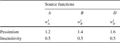
In this scenario, we examine investor II, who is an expert in the food industry. The researcher has elicited the investor’s source functions, as shown in Table 2. The parameters for sources A and B are the same as in the previous scenario. For sources C and D, the investor also exhibits a home bias, with a preference for C over D, but exhibits more sensitivity toward these sources than toward A and B, possibly due to their expertise in the food industry. The analyst questions whether the magnitude of the home bias is the same between A and B as between C and D. The difference in the pessimism parameters is the same (0.2) between A and B as between C and D. The difference in the sensitivity parameters is also the same (0) between A and B as between C and D. Thus, looking at “differences of differences” leads to the conclusion that the magnitude of the home bias is the same between A and B as between C and D.

Table 2 Scenario 2. Differences in source functions within individual

	Source functions
	A	B	C	D
	$w_{A}^{II}$	$w_{B}^{II}$	$w_{C}^{II}$	$w_{D}^{II}$
Pessimism	1.2	1.4	1.2	1.4
Insensitivity	0.5	0.5	0.7	0.7

However, investor II is willing to give up on more gain probabilities for betting on A rather than B than for betting on C rather than D (see Fig. 1 in Sect. 3.2). In other words, the source premium is larger between A and B than between C and D. This is because the investor is less sensitive to probability changes for A than for C, thus requiring a larger ambiguity premium to compensate for the same difference in weight. This example illustrates that differences in source function parameters cannot be compared across pairs of sources, even within an individual, since differences in source functions correspond to differences in “weight,” which have different values depending on the sensitivity toward the sources being considered.

2.3.3 Scenario 3: Comparing differences in parameters of non-linear specifications

We now focus on investor I and consider sources A, B, and D (see Table 3). The analyst wants to compare the preference between A and B (local vs. foreign in the investor’s domain of expertise) to the difference between B and D (expertise vs. non-expertise for foreign sources). In this case, the differences in the pessimism parameters between A and B and between B and D are the same (0.2). Here again, one should not conclude that the source premium that investor II is willing to pay for betting on A rather than B is the same as the premium that the investor is willing to pay for betting on B rather than D. In fact, the premium is larger for the former than for the latter. The reason for this is the nonlinearity of the source functions. A difference in the pessimism parameters of 0.2 does not have the same effect between 1.2 and 1.4 as it does between 1.4 and 1.6. This scenario illustrates how difference-in-differences in parameters of non-linear specifications cannot be easily used to analyze differences in source dependence.

Table 3 Scenario 3. Differences in parameters of non-linear specifications

	Source functions
	A	B	D
	$w_{A}^{I}$	$w_{B}^{I}$	$w_{D}^{I}$
Pessimism	1.2	1.4	1.6
Insensitivity	0.5	0.5	0.5

3 A function for measuring source dependence

In this section, we introduce a function $ϕ$ , referred to as a p(robability)matcher, which enables direct measurement of the source dependence of preferences between two natural sources. We then show that such functions can be estimated using either matching probabilities (MP), which assess attitudes toward a source on the scale of probabilities, or certainty equivalents (CE), which assess attitudes toward a source on the scale of outcomes.

3.1 A direct measure of source dependence

We introduce a function $ϕ$ that enables the quantification of source dependence and allows for comparisons between individuals and (pairs of) sources. We consider two natural sources, A and B, and their functions $w_{A}$ and $w_{B}$ . The function $ϕ_{AB}$ is defined such that $w_{B} = w_{A} \circ ϕ_{AB}$ (i.e., $ϕ_{AB} = w_{A}^{- 1} \circ w_{B}) .$ It is strictly increasing, satisfies $ϕ_{AB} (0) = 0$ and $ϕ_{AB} (1) = 1$ , and maps probabilities $μ_{B}$ of events $E_{B}$ generated by the source B to probabilities $μ_{A}$ of events $E_{A}$ generated by the source A as follows: for any event $E_{B}$ generated by source B with a subjective probability $μ_{B}$ , all the events $E_{A}$ generated by source A with a subjective probability $μ_{A} = ϕ_{AB} (μ_{B})$ are such that the decision maker is indifferent between betting on $E_{B}$ and $E_{A}$ .

The comparison of $μ_{B}$ and $μ_{A}$ characterizes source preference between the two sources. Deviations of $ϕ_{AB}$ from identity directly characterize source dependence: A is strictly preferred to B if $ϕ_{AB} (μ) < μ .$ In turn, $μ - ϕ_{AB} (μ)$ represents the source premium of source A over source B, i.e., the decrease in likelihood the decision maker is willing to accept in order to bet on source A instead of source B. Because the source premium is measured on the scale of “a-neutral” probabilities, it is independent of risk and ambiguity attitudes. Therefore, the transformation function $ϕ_{AB}$ offers a direct measure of source preference for A over B that can be compared across individuals and (pairs of) sources. Inversely, the source preference for B over A is captured by $ϕ_{BA} = ϕ_{AB}^{- 1}$ .

We now illustrate how the shape of the function $ϕ$ relates to choice patterns revealing source dependence. We call A-event an event generated by source A and B-event an event generated by source B. Suppose there exists a probability $μ$ such that $ϕ_{AB} (μ) < μ$ and $ϕ_{AB} (1 - μ) < (1 - μ)$ . Then, for all events $E_{A}$ with a subjective probability $μ^{'}$ such that $μ > μ^{'} > ϕ_{AB} (μ)$ , we will observe that $x_{E_{A}} y ≻ x_{E_{B}} y$ . This is because $μ^{'} > ϕ_{AB} (μ)$ implies that $w_{A} (μ^{'}) > w_{B} (μ)$ . Moreover, we will also observe that $x_{E_{A}^{c}} y ≻ x_{E_{B}^{c}} y$ , since $ϕ_{AB} (1 - μ) < 1 - μ < 1 - μ^{'}$ implies that $w_{A} (1 - μ^{'}) > w_{B} (1 - μ) .$ In other words, it is possible to find A-events such that, for all B-events with probability $μ$ , the decision maker prefers to bet on A-events instead of B-events and also prefers to bet against A-events instead of against B-events.

Another key dimension of source preference is comparative sensitivity (Tversky & Fox, Reference Tversky and Fox1995), which can be illustrated by the following example. Suppose there are two disjoint events $E_{A}$ and $E_{A}^{'}$ generated by A, and two disjoint events $E_{B}$ and $E_{B}^{'}$ generated by B such that $x_{E_{B}} y \sim x_{E_{A}} y$ and $x_{E_{B}^{'}} y \sim x_{E_{A}^{'}} y$ for all $x > y$ . If we also observe that $x_{E_{B} \cup E_{B^{'}}} y ≺ x_{E_{A} \cup E_{A^{'}}} y$ , then the decision maker is less sensitive to probability changes for B than for A. We say the decision maker exhibits less relative sensitivity (or equivalently, more relative insensitivity) toward B than toward A. This pattern is captured by the curvature of the function $ϕ$ . Indeed, $x_{E_{B}} y \sim x_{E_{A}} y$ and $x_{E_{B}^{'}} y \sim x_{E_{A}^{'}} y$ imply that $μ_{A} = ϕ_{AB} (μ_{B})$ and $μ_{A}^{'} = ϕ_{AB} (μ_{B}^{'})$ , respectively. Thus, $x_{E_{B} \cup E_{B^{'}}} y ≺ x_{E_{A} \cup E_{A^{'}}} y$ implies that $ϕ_{AB} (μ_{B}) + ϕ_{AB} (μ_{B}^{'}) > ϕ_{AB} (μ_{B} + μ_{B}^{'})$ . The function exhibits subadditivity for some probabilities.

Overall, the two dimensions of the function $ϕ$ can be interpreted as follows: the elevation captures relative preference (“more or less preference for B than for A”), and the slope captures relative (in)sensitivity (“more or less insensitivity for B than for A”). For example, an inverse S-shaped $ϕ_{AB}$ function can generate both a relative preference for A and a relative insensitivity toward B.

3.2 Comparing attitudes across sources and individuals using $ϕ$

We illustrate the pmatcher $ϕ$ using the three scenarios described in Sect. 2.3.

In the first scenario, the two investors have the same source functions for stocks A and B, and both exhibit a preference for A over B. The pmatchers $ϕ_{AB}$ of the two investors are shown on the left panel of Fig. 1. When $μ_{A} < μ_{B}$ , the decision maker exhibits a preference for source A over source B and is willing to accept a reduction in the winning probability $(μ_{B} - μ_{A})$ to bet on the event generated by source A instead of the one generated by source B with probability $μ_{B}$ .Footnote ⁸ For both investors, $ϕ_{AB} (x) < x$ for all values of x, indicating a preference for source A over source B. Moreover, the magnitude of the source dependence between A and B, capturing the home bias, is the same for the two investors. The pmatcher enables a direct comparison between individuals. Although the two investors have different risk attitudes (investor I does not distort objective probabilities, while investor II exhibits an inverse S-shaped probability weighting), the figure correctly reports that they have the same function $ϕ_{AB}$ .

The second scenario, shown in the middle panel of Fig. 1, displays a stronger deviation from linearity for $ϕ_{AB}$ than for $ϕ_{CD}$ , indicating a stronger source dependence for A over B than for C over D. The pmatcher captures this larger magnitude of source dependence, which was not detected by comparing the (differences in) source functions, as seen in Sect. 2.3.

In the third scenario, the deviation from linearity is stronger for $ϕ_{AB}$ than for $ϕ_{BD}$ , indicating a stronger source preference for A over B than for B over D. As we saw in Sect. 2.3, comparisons of (differences in) parameters between sources would fail to capture this effect due to the nonlinearity of the source function specification.

These scenarios illustrate how the pmatcher helps overcome the difficulties faced when comparing ambiguity attitudes toward different sources, allowing for comparison across individuals and sources.

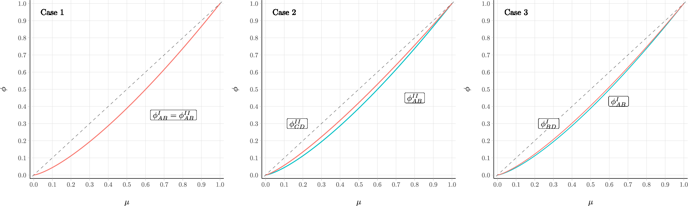
Fig. 1 Illustration of the pmatchers for the three scenarios of Sect. 2.3

3.3 Estimating $ϕ$ from matching probabilities

As introduced earlier, the method developed by Dimmock et al. (Reference Dimmock, Kouwenberg and Wakker2016b) consists of fixing an outcome $x > 0$ and measuring a series of matching probabilities $M_{S}$ such that $(x, M_{S}, 0) \sim (x, E_{S}, 0)$ , where $E_{S}$ are events generated by S for which the a-neutral probabilities $μ (E_{S}) = λ_{S}$ are known. The analysis then consists of eliciting an ambiguity function $m_{S}$ that maps the probabilities $μ (E_{S}) = λ_{S}$ onto the matching probabilities $M_{S}$ :

(6)

\begin{matrix} m_{S} (λ_{S}) = M_{S} . \end{matrix}

Under standard assumptions of monotonicity and continuity, the ambiguity function $m_{S}$ is strictly increasing and satisfies $m_{S} (0) = 0$ and $m_{S} (1) = 1$ . According to Eq. (5), $m_{S} = w^{- 1} \circ w_{S}$ . The function $ϕ_{AB}$ between two sources A and B, with ambiguity functions $m_{A}$ and $m_{B}$ , can be obtained as follows:

\begin{matrix} m_{B} = w^{- 1} \circ w_{B} = w^{- 1} \circ w_{A} \circ ϕ_{AB} = m_{A} \circ ϕ_{AB}, \end{matrix}

hence,

\begin{matrix} ϕ_{AB} = m_{A}^{- 1} \circ m_{B} . \end{matrix}

The function $ϕ_{AB}$ relies on a direct comparison of ambiguity functions $m_{A}$ and $m_{B}$ , with no need to measure the weighting function for risk w or the source functions $w_{A}$ and $w_{B}$ .

3.4 Estimating $ϕ$ from certainty equivalents

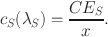
Suppose that we fix an outcome $x > 0$ and measure, for each source S, a series of certainty equivalents $C E_{S}$ such that $C E_{S} \sim (x, E_{S}, 0)$ , where $E_{S}$ are events generated by S, for which the a-neutral probabilities $μ (E_{S}) = λ_{S}$ are known. The method then consists of estimating a function $c_{S}$ that maps these probabilities $μ (E_{S}) = λ_{S}$ to the normalized certainty equivalents $C E_{S}$ :

(7)

\begin{matrix} c_{S} (λ_{S}) = \frac{C E_{S}}{x} . \end{matrix}

For parallelism with the ambiguity function, we refer to $c_{S}$ as an uncertainty function. Under standard assumptions of monotonicity and continuity, the uncertainty function $c_{S}$ is strictly increasing and satisfies $c_{S} (0) = 0$ and $c_{S} (1) = 1$ . According to Eq. (5), and after rescaling the utility such that $U (0) = 0$ and $U (x) = 1$ , $c_{S} = \frac{U^{- 1} \circ w_{S}}{x}$ . Assuming that utility is source-independent (an assumption generally made in applications of the source model and empirically supported by Abdellaoui et al., Reference Abdellaoui, Baillon, Placido and Wakker2011), differences in uncertainty functions $c_{S}$ across sources reveal differences in source functions. The function $ϕ_{AB}$ between two sources A and B, with uncertainty functions $c_{A}$ and $c_{B}$ , can be obtained as follows:

\begin{matrix} c_{B} = \frac{U^{- 1} \circ w_{B}}{x} = \frac{U^{- 1} \circ w_{A} \circ ϕ_{AB}}{x} = c_{A} \circ ϕ_{AB}, \end{matrix}

hence,

\begin{matrix} ϕ_{AB} = c_{A}^{- 1} \circ c_{B} . \end{matrix}

Therefore, it is possible to estimate $ϕ_{AB}$ from certainty equivalents with no need to control for the utility function. In this paper, we do not interpret the uncertainty functions on their own. We instead use them as a measurement tool for assessing source dependence.

3.5 Comments on $ϕ$

Overall, $ϕ_{AB}$ can be estimated simply from either matching probabilities or certainty equivalents. It does not require measuring or controlling for the utility, the weighting function for risk, or even the source functions. Therefore, it can be estimated from a smaller number of choices and avoid error propagation due to the measurement of utility and source (or risk) weighting functions.

The characterization of source dependence is independent of risk attitudes (related to $u$ and $w$ ) and ambiguity attitudes (related to the difference between $w_{A}$ and $w$ or between $w_{B}$ and $w$ ). Instead, it relates to the differences in attitudes across sources. A linear $ϕ$ does not necessarily mean that decision makers are risk neutral or ambiguity neutral for the two sources, only that they exhibit the same attitude for the two sources. Conversely, there may be source dependence even if decision makers are risk neutral or ambiguity neutral for one of the two sources. Therefore, the introduction of source dependence, as measured by the function $ϕ$ , enlarges the scope of analysis of attitudes toward natural sources of uncertainty beyond the concept of risk and ambiguity attitudes.

Eventually, when A is a risky source (R), $w_{B} = w \circ ϕ_{RB}$ and $ϕ_{RB} = w^{- 1} \circ w_{B}$ . In this case, the transformation function $ϕ_{RB}$ corresponds to the ambiguity function proposed by Dimmock et al. (Reference Dimmock, Kouwenberg and Wakker2016b) for capturing ambiguity attitudes. To summarize, the function $ϕ$ generalizes the approach of Dimmock et al. (Reference Dimmock, Kouwenberg, Mitchell and Peijnenburg2016a) in two ways: it extends the approach for capturing source dependence between natural sources, and it allows measurement using not only matching probabilities but also certainty equivalents.

4 Empirical implementation

4.1 Data

We conducted three studies to empirically test our method, including one that used an existing dataset (Study A) and two original experiments (Studies B and C). To test the generality of our method, we selected experimental designs that employed various approaches to evaluating prospects (certainty equivalents vs. matching probabilities) and identifying beliefs. As discussed in Sect. 2, studying attitudes toward natural sources requires accounting for beliefs that are not necessarily uniform. We demonstrate that our method can be applied with two commonly used choice-based methods to disentangle ambiguity attitudes and beliefs: the exchangeable-events method (Studies A and B) and the belief-hedging method (Study C).

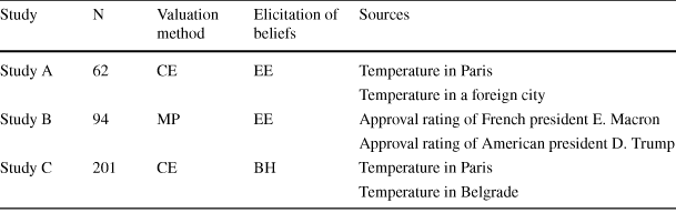
The studies used different experimental procedures, with individual interviews and random incentives used in Studies A and B and an online experiment with hypothetical choices used in Study C. In each study, one source was local and arguably more familiar to the subjects than the other. We used this local source as the reference source. We summarize the characteristics of each dataset in Table 4 and provide details for all three studies below. Instructions for experiments B and C are included in Online Appendix D.

Table 4 Summary of the three datasets

Study	N	Valuation method	Elicitation of beliefs	Sources
Study A	62	CE	EE	Temperature in Paris
Study A	62	CE	EE	Temperature in a foreign city
Study B	94	MP	EE	Approval rating of French president E. Macron
Study B	94	MP	EE	Approval rating of American president D. Trump
Study C	201	CE	BH	Temperature in Paris
Study C	201	CE	BH	Temperature in Belgrade

EE stands for exchangeable events and BH for belief hedging

4.1.1 Study A

For this study, we used data from Abdellaoui et al. (Reference Abdellaoui, Baillon, Placido and Wakker2011) on two natural sources S, the temperature in Paris ( $S = A$ ) and the temperature in a foreign city ( $S = B$ ). For each source, participants’ beliefs were measured prior to eliciting their attitudes toward ambiguity.

Measurement of beliefs: Participants’ beliefs about the sources were measured using the approach developed by Baillon (Reference Baillon2008) based on exchangeable events (see Sect. 2). For each source S, a sequential process was used to build a series of five events $E_{k, S}$ with probabilities $μ_{k} \in (1 / 8, 1 / 4, 1 / 2, 3 / 4, 7 / 8)$ . Abdellaoui et al. (Reference Abdellaoui, Baillon, Placido and Wakker2011) provide more details about the procedure.

Evaluation of prospects: With these events (for which the researchers knew the a-neutral probability) at hand, the certainty equivalents $C E_{k, S}$ of five prospects $(1000, E_{k, S}, 0)$ were measured for each source. These CEs allowed us to assess the uncertainty function $c_{S}$ since $c_{s} (μ_{k, S}) = \frac{C E_{k, S}}{1000}$ .Footnote ⁹

Procedure: 62 participants participated in individual computer-based interviews. Random incentives were implemented for half of the participants (real-incentive treatment), whereas the other half made hypothetical choices (hypothetical treatment). For the real-incentive treatment, one of the 31 participants was randomly selected at the end of the experiment, and one of their choices was randomly selected to determine their monetary gain. The payment was made three months after the experiment, once the uncertainty was resolved (Abdellaoui et al., Reference Abdellaoui, Baillon, Placido and Wakker2011 provide more details).Footnote ¹⁰

4.1.2 Study B

For this study, we followed a similar design to Study A, but with different sources and a distinct valuation approach of ambiguous prospects. In contrast to Study A, we evaluated ambiguous prospects using matching probabilities (MPs) instead of certainty equivalents (CEs). We used two sources S, the approval ratings of French President Emmanuel Macron ( $S = A$ ) and US President Donald Trump ( $S = B$ ).Footnote ¹¹ Each of these variables ranged between 0 and 100 percent and was revealed one month after the experiment.Footnote ¹²

Measurement of beliefs: We used the exchangeable-events method, as in Abdellaoui et al. (Reference Abdellaoui, Baillon, Placido and Wakker2011) and Study A, to elicit a series of events $E_{k, S} = [0, v_{k, S}]$ generated by sources S, with a-neutral probabilities $μ (E_{k, S}) \in (1 / 8, 1 / 4, 1 / 2, 3 / 4, 7 / 8)$ . Values $v_{k, S}$ represented the percentages of approval ratings and were measured with a precision of one percentage point.

Evaluation of prospects: We measured ambiguity attitudes using matching probabilities. For each source, we measured the matching probabilities $m p_{k, S}$ of prospects $(100, E_{k, S}, 0)$ with a precision of 0.01. This allowed us to assess the ambiguity function $m_{S}$ because $m_{s} (μ_{k, S}) = m p_{k, S}$ .

Both beliefs and attitudes rely on the measurement of indifference values, which we elicited using choice lists. We used a bisection procedure to complete these lists (see Abdellaoui et al., Reference Abdellaoui, Kemel, Panin and Vieider2019). When a list was completed, the participants reviewed all the choices from the list and were able to make changes if desired. Participants then had to confirm the whole list for the software to move to the next choice list.

Procedure: We recruited 94 participants to take part in a 1-h individual computer-based interview for a compensation of €10. Participants started by watching a 10-min video describing the experiment. Then they completed a survey with comprehension questions to identify those who required additional clarifications from the research assistants. The experiment started with several practice questions to familiarize participants with the software. Participants then completed the belief task and the ambiguity task for one of the two sources before moving on to the second source. For each source, the belief task always preceded the ambiguity task. The order of the questions in the ambiguity task was randomized.

Real incentives were used, and the procedure was explained in the instructions (see Online Appendix D). Each participant received an envelope and was informed that each envelope had a 10% chance of containing a winning ticket. At the end of the session, participants opened the envelopes to see if they had received the winning ticket, which would allow one of their choices to be played for real. A computer program randomly selected one of the choices made by the selected participants. During the instructions, participants were informed that all of their choices could be selected and played for real. The selected participants could gain up to €100 extra. Eight participants were randomly selected for one of their choices to be played out for real. Three of them earned €100 extra, while the others did not earn an extra bonus. Overall, the average payment was €13.2 per hour.

4.1.3 Study C

In this study, we measured beliefs and attitudes jointly using certainty equivalents and the belief-hedging method (Baillon et al., Reference Baillon, Bleichrodt, Keskin, L’Haridon and Li2017; Li et al., Reference Li, Turmunkh and Wakker2019).

Evaluation of prospects: We considered two sources S, the temperature, in celsius degrees, in a local city, Paris, France (source $S = A$ ), and a foreign city, Belgrade, Serbia (source $S = B$ ). For each source S, we created an exhaustive partition of mutually exclusive events $E_{1, S}, E_{2, S}, E_{3, S}$ and measured CEs for all prospects $(20, E_{k, S}, 0)$ , where $E_{k, S} \in {E_{1, S}, E_{1, S}^{c}, E_{2, S}, E_{2, S}^{c}, E_{3, S}, E_{3, S}^{c})$ . The three events were $E_{1, S} = (- \infty, 18]$ , $E_{2, S} =] 18, 22]$ , and $E_{3, S} =] 22, + \infty)$ and their complementary events $E_{1, S}^{c} =] 18, + \infty),$ $E_{2, S}^{c} = (- \infty, 18] \cup] 22, + \infty)$ , and $E_{3, S}^{c} = (- \infty, 22]$ . We elicited CEs using a bisection method with a precision of €1.

Procedure: We recruited a sample of 201 participants from the INSEAD Behavioral Lab subject pool and conducted the experiment online using hypothetical choices. To improve the quality of the data despite the absence of incentives and online data collection, we used an application designed specifically for this purpose. The app detected the size of the user’s screen to prevent completion of the study on smartphones and froze the choice buttons for 2 s for each question to prevent rushing completion.

4.2 Estimation strategy

4.2.1 Errors specification and likelihood function

We used a unified statistical approach to measure source dependence between two sources $s \subset {A, B}$ in the available datasets. In the three experiments, our measurement followed an equation of type

\begin{matrix} y_{i, k, s} = & f_{i} (μ_{i, k, s}) if s=A \\ = & f_{i} \circ ϕ_{i} (μ_{i, k, s}) if s = B \end{matrix}

where $y_{i, k, s}$ is the valuation (either a MP or a CE) by subject i of a prospect k involving event $E_{i, k, s}$ with probability $μ_{i, k, s}$ , f is either an ambiguity or uncertainty function, and $ϕ$ is a pmatcher.

We assumed that subjects made decision errors, such that the measured indifference $y_{i, k, s}^{⋆}$ followed $y_{i, k, s}^{⋆} = y_{i, k, s} + ϵ_{i, s}$ where $ϵ_{i, s} \sim N (0, σ_{i, s}^{2}$ ). Hence, we accounted for heteroscedasticity across sources and individuals. Indifferences were measured with a precision $η$ such that the likelihood of each observation followed

\begin{matrix} π (y_{i, k, s} | θ_{i,}, μ_{i, k, s}) = & p (y_{i, k, s}^{⋆} - \frac{η}{2} < y_{i, k, s} + ϵ_{i, s} < y_{i, k, s}^{⋆} + \frac{η}{2}) \\ = & p (y_{i, k, s}^{⋆} - \frac{η}{2} - y_{i, k, s} < ϵ_{i, s} < y_{i, k, s}^{⋆} + \frac{η}{2} - y_{i, k, s}) \\ = & Ψ (\frac{y_{i, k, s}^{⋆} - y_{i, k, s} + \frac{η}{2}}{σ_{i, s}}) - Ψ (\frac{y_{i, k, s}^{⋆} - y_{i, k, s} - \frac{η}{2}}{σ_{i, s}}) \end{matrix}

where $θ_{i}$ is the vector of function parameters $a_{i}$ and $b_{i}$ (the parameters of $f_{i}$ for the domestic source, taken as the reference source), $α_{i}$ and $β_{i}$ (the parameters of the function $ϕ_{i}$ ), and $μ_{i, k, s}$ (the beliefs). The cumulative function of the normal distribution is denoted $Ψ$ . In Studies A and B, beliefs were measured separately from (and before) attitudes. In contrast, Study C utilized belief hedging, where beliefs were estimated jointly with other parameters (see the details in Online Appendix B).

The likelihood for a given individual i is

\begin{matrix} l (θ_{i}) = \prod_{s} \prod_{k} π (y_{i, k, s}, θ_{i,}, μ_{i, k, s}) . \end{matrix}

This likelihood specification aims to elicit the parameters of the function f that captures attitudes toward one of the two sources (taken as the reference) and, more importantly, the parameters of the transformation function $ϕ$ that captures source dependence.

4.2.2 Parametric specifications

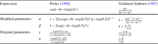
In our analyses, we used parametric specifications for the functions f and $ϕ$ . We considered two popular, non-linear, two-parameter specifications for the function f (see Table 5): the Goldstein Einhorn (Reference Goldstein and Einhorn1987, hereafter GE) and the Prelec (Reference Prelec1998). Parametric specifications have been commonly used to model probability-weighting functions (Bruhin et al., Reference Bruhin, Fehr-Duda and Epper2010), ambiguity functions (Li et al., Reference Li, Müller, Wakker and Wang2017), and even uncertainty functions (l’Haridon & Vieider, Reference L’Haridon and Vieider2019). In all these applications, the two parameters, relating respectively to elevation and curvature, have behavioral interpretations. The parameter capturing the global elevation of the function (denoted $δ$ ) is interpreted in terms of optimism, and the one measuring the curvature of the function (denoted $γ$ ) is interpreted in terms of sensitivity toward changes in probabilities. These non-linear specifications usually offer a better goodness of fit than the neo-additive specification (Li et al., Reference Li, Müller, Wakker and Wang2017). However, there are limitations to their use. First, the interpretation of the parameters is different for each specification. For example, Li et al. (Reference Li, Müller, Wakker and Wang2017, p. 10) have noted that “in Prelec’s family, the insensitivity parameter $[γ]$ overlaps partly with the aversion parameter $[δ]$ , also capturing some aversion.” Second, the interpretation of differences in parameters varies across specifications. For example, the parameter $δ$ decreases with increasing elevation in the case of the Prelec specification, but it increases with increasing elevation in the case of the GE specification. Third, the parameters of these specifications take non-negative values. When random coefficient estimation methods are used, these parameters are generally assumed to be log-normally distributed, which requires cumbersome transformations for reporting their estimates and inferences on their mean and variance in a sample.

Expressing these two specifications with parameters that have the same range and interpretation and can take both positive and negative values is therefore desirable. We propose such a reparametrization of the GE and the Prelec specifications using two parameters $β = 1 - 2 ϕ (0.5)$ and $α = 1 - \frac{\partial ϕ}{\partial μ} (0.5)$ . We use $β$ to denote the global elevation parameter, which captures the overall elevation of the plot, and $α$ to denote the global sensitivity parameter, which governs curvature (e.g., the inverse-S shape of the plot). Importantly, while simplifying the interpretation of the results, this reparametrization does not create any loss of generality.

Applying this reparametrization to pmatchers, the first parameter $β$ captures the relative preference for source A over source B. As shown in Fig. 2, when $β > 0$ (blue curves), the subject exhibits a preference for source A over source B, whereas when $β < 0$ (red curves), the subject exhibits a preference for source B over source A. In addition, the value $β / 2$ represents the source premium of source A over source B in the middle of the probability interval. It reflects the decrease in likelihood the decision maker is willing to accept to bet on source A instead of source B. When $ϕ (0.5) = 0.5$ , $β / 2 = 0$ , which indicates no source premium. Regardless of the underlying reason for the preference, it can be interpreted as a higher level of optimism toward one source compared to the other. We will use the terms relative optimism and relative preference interchangeably: when $β > 0$ (resp. $β < 0$ ), we say that there is a relative preference, or relative optimism, toward A (resp. B).Footnote ¹³

The second parameter $α$ relates to the slope (i.e., the derivative) of the function $ϕ$ at probability 0.5. It captures the rate of substitution between the probabilities generated by A and the probabilities generated by B. Starting from 0.5, an increase of $ϵ$ in probability generated by B has the same effect as an increase of $(1 - α) ϵ$ in probability generated by A. Therefore, the parameter $α$ can be interpreted in terms of relative insensitivity. When $α > 0$ , there is more insensitivity toward B than toward A, and we say that there is relative insensitivity toward B. When $α < 0$ , there is more sensitivity toward B than toward A, and we say that there is relative insensitivity toward A.

An interesting and convenient property is that these parameters can be directly computed from the original parameters of the two non-linear specifications considered in this paper (see Table 5 for the mapping between these parameters and the original ones). Importantly, while the parameters can be interpreted with reference to the value of the function or its derivative for probability 0.5, they are not estimated from the behavior of the function in the middle of the probability interval alone. Instead, they depend on the behavior of the function over the whole interval, like any other parametric specification. In this regard, the function estimated using our parameters is one-to-one related to the function estimated using the original parameters. However, the re-parametrization allows for an easier interpretation of the function parameters and their heterogeneity. In particular, the parameters have the same interpretation (regarding the elevation and the slope of the function), regardless of the chosen specification.Footnote ¹⁴

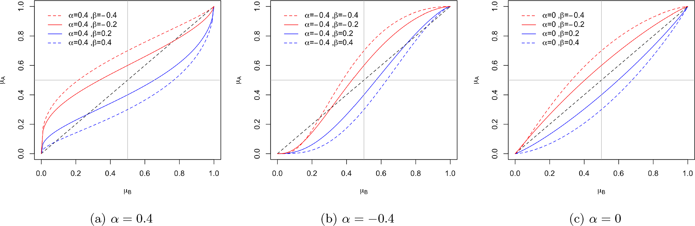
Fig. 2 Illustration of the function $ϕ$

Table 5 Specifications and their re-parametrization

Expression		Prelec (Reference Prelec1998)	Goldstein Einhorn (Reference Goldstein and Einhorn1987)
Expression		$e x p (- δ {(- l o g (p))}^{γ})$	$\frac{δ p^{γ}}{δ p^{γ} + {(1 - p)}^{γ}}$
Modified parameters	$α$	$1 - 2 δ γ e x p (- δ {(- l o g (0.5))}^{γ}) {[- l o g (0.5)]}^{γ - 1}$	$1 - \frac{δ γ p^{γ - 1} {(1 - p)}^{γ - 1}}{{(δ p^{γ} + {(1 - p)}^{γ})}^{2}}$
Modified parameters	$β$	$1 - 2 e x p (- δ {(- l o g (0.5))}^{γ})$	$1 - 2 \frac{δ}{δ + 1}$
Original parameters	$γ$	$\frac{l o g (0.5) (1 - α)}{(1 - β) l o g (0.5 (1 - β))}$	$\frac{1 - α}{(1 + β) (1 - β)}$
Original parameters	$δ$	$\frac{- l o g [0.5 (1 - β)]}{{[- l o g (0.5)]}^{γ}}$	$\frac{1 - β}{1 + β}$

4.2.3 Accounting for preference heterogeneity

At the aggregate level, all the subjects are assumed to have the same preferences, i.e., $θ_{i}$ did not depend on the index i. In particular, this means that the preferences of all the subjects are the same for the reference source and reveal the same pattern of source dependence. However, this assumption may be unrealistic, as individual-level parameters are likely to vary across subjects. Estimating individual-level parameters requires a large amount of data and may not be of interest to researchers, who are usually interested in the distribution of parameters in the sample rather than the behavior of a specific individual. To measure the distribution of parameters in our samples, we use a random-coefficient model where source dependence (captured by parameters $α_{i}$ and $β_{i}$ ) is randomly distributed across subjects. We assume that the parameters of ambiguity or uncertainty functions for the reference source are randomly distributed.

The mean (standard deviation) of the distributions of relative insensitivity and relative optimism parameters are denoted as $\bar{α}$ and $\bar{β}$ ( $σ_{α}$ and $σ_{β}$ ). The random coefficient models are estimated using Hierarchical Bayes (HB) simulations, which have recently been shown to be suitable for estimating risk models (Murphy & ten Brincke, Reference Murphy and ten Brincke2017; Baillon et al., Reference Baillon, Bleichrodt and Spinu2020). To do so, we used the RSGHB R package, with priors corresponding to linear uncertainty or ambiguity functions with virtually no heterogeneity. Such priors correspond to rational representative agent models (ambiguity-neutral or uncertainty-neutral attitudes) with no between-subject heterogeneity and no source dependence. Our choice of priors based on rational-choice models reflects a conservative approach that plays “against” our results, which revealed non-linear and heterogeneous functions with heterogeneous patterns of source dependence.

5 Results

This section presents the results of the empirical implementation of our econometric set-up for the three studies. For each study, we report the econometric estimations of the means and standard deviations of the parameters of the function $ϕ_{AB}$ (see Table 6). The descriptive statistics of studies B and C are provided in Online Appendix A.Footnote ¹⁵ We focus on the results obtained with the Prelec specification, as it is compatible with the parametric approaches used for modeling both uncertainty and ambiguity functions.Footnote ¹⁶ The results obtained with the Goldstein-Einhorn specification were similar (see Online Appendix C). We report our results focusing on the two dimensions of the pmatcher $ϕ$ : elevation, which captures relative preference, and curvature, which captures relative sensitivity.

The pmatchers were estimated using a Hierarchical Bayes method that accounts for individual heterogeneity of parameters. For each study, we display both the modal patterns and the heterogeneity (see Figs. 3, 4, 5). The left-hand panel plots the median pmatcher and its interquartile range. The other two panels show the outputs of Bayesian estimations for each of the two parameters of the pmatcher. Specifically, we plot the cumulative distributions of individual parameters and their precision (credible intervals). Like in most studies, there is no particular interest in knowing the parameters of each specific individual. Instead, we are interested in the distribution of individual parameters in the sample. We thus focus our analysis on the estimated mean and variance of the parameters in our subject samples (Table 6).Footnote ¹⁷ The distributions corresponding to the estimated means and variances are plotted in plain lines on the middle and right panels of Figs. 3, 4, 5.Footnote ¹⁸

Table 6 Summary of HB estimations—Studies A, B, and C

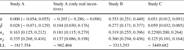
	Study A	Study A (only real incentives)	Study B	Study C
$\bar{α}$	0.000 [− 0.054; 0.055]	− 0.205 [− 0.286; − 0.096]	0.353 [0.251; 0.449]	0.051 [0.012; 0.091]
$\bar{β}$	0.028 [− 0.071; 0.129]	0.104 [0.030; 0.176]	0.277 [0.171; 0.377]	0.059 [0.032; 0.085]
$σ_{α}$	0.163 [0.125; 0.212]	0.181 [0.115; 0.279]	0.319 [0.255; 0.396]	0.229[0.200; 0.264]
$σ_{β}$	0.335 [0.268; 0.416]	0.137 [0.086; 0.198]	0.360 [0.294; 0.436]	0.125 [0.101; 0.164]
LL	− 1817.354	− 982.404	− 3313.293	− 3449.682

95% credible intervals between brackets

5.1 Study A

Study A compared attitudes toward temperature in a local city (Paris, France) and temperature in a foreign city, which differed for each subject. The left panel of Fig. 3 displays the quartile behavior (median and interquartile range) of the estimated function $ϕ_{AB}$ .

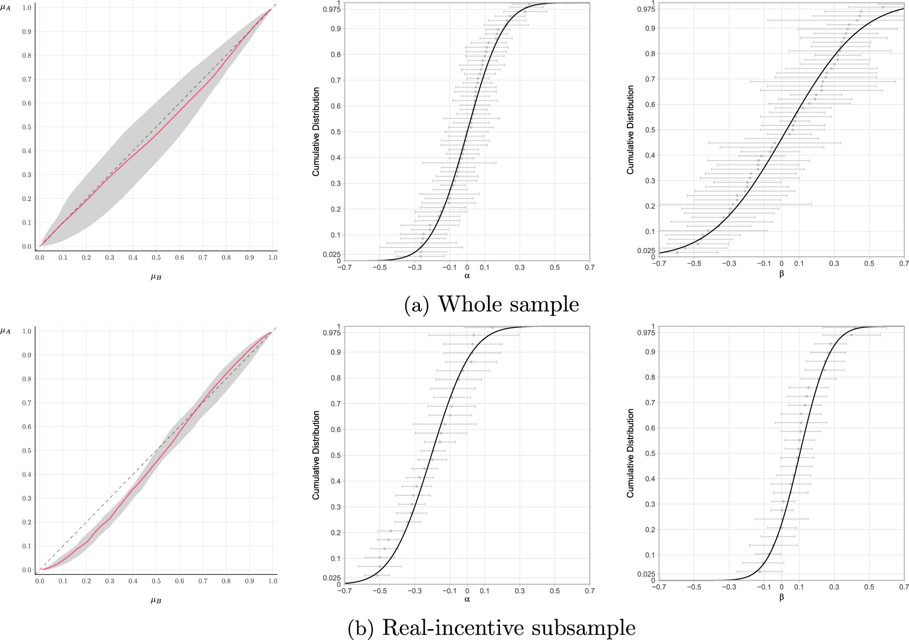
Fig. 3 pmatcher $ϕ_{AB}$ and estimated distributions of its two parameters (Study A)

We found no average source dependence as the 95% credible interval (hereafter CI) of the two parameters of the function $ϕ_{AB}$ ( $\bar{α}$ and $\bar{β}$ ) included 0. However, the middle and right panels of Fig. 3 show large heterogeneity across individuals. The standard deviation of the elevation parameter ( $σ_{β} = 0.33$ ) suggested that $β$ was greater than 0.3, in absolute value, for one-third of the sample.Footnote ¹⁹ In other words, one-third of the subjects behaved as if they inflated or deflated a 0.5 winning event probability by at least 0.15, depending on their source preference. We also found heterogeneity in the sensitivity dimension of source dependence, indicating that relative sensitivity to the sources was also heterogeneous in the sample. This illustrates the importance of addressing heterogeneity in parameters, as average results can mask pronounced individual effects that cancel out at the aggregate level.

Following the analyses performed in the original paper (Abdellaoui et al., Reference Abdellaoui, Baillon, Placido and Wakker2011), we estimated the distributions of parameters focusing on the group with real incentives. In this subsample, estimated means show evidence of source dependence. The parameter $\bar{β}$ was positive (95% CI = [0.030; 0.176]), indicating that subjects exhibited a preference for the local source over the foreign source on average. The re-parametrization offers an easy interpretation of this parameter. The source premium in the middle of the likelihood interval was equal to 0.05 (i.e., $\bar{β} / 2$ ). In other words, the average subject was willing to forego a 0.05 winning probability in order to bet on an event generated by the local source rather than an event generated by the foreign source with a probability of 0.5.

The average insensitivity parameter $\bar{α}$ for the group with real incentives was negative (95% CI = $[- 0.286; - 0.096]$ ). This parameter can be interpreted in terms of relative (in)sensitivity. Participants in the real incentives group were more sensitive to the foreign source than to the local source. According to the mean insensitivity parameter $\bar{α} = - 0.2$ , an increase in the probability of $ϵ$ from 0.5 in source B has the same impact as an increase of $1.2 ϵ$ points from 0.5 in source A.Footnote ²⁰ This finding is somewhat surprising, given that a greater degree of likelihood insensitivity is typically interpreted as indicating higher perceived ambiguity (Baillon et al., Reference Baillon, Huang, Selim and Wakker2018). Notably, this observation is in contrast to the results presented in Studies B and C.

Overall, Study A confirmed the source dependence of preferences. In the real-incentive subsample, subjects exhibited a preference for the local source over the foreign source. Furthermore, changes in probabilities did not have the same effect on the two sources; there was less insensitivity to changes in the foreign source than in the local one. This study also revealed considerable heterogeneity in source dependence and provided evidence of pronounced source dependence for a sizable part of the sample. Interestingly, despite considerable source dependence at the individual level in the whole sample (i.e., when pooling incentivized and non-incentivized groups), the effects canceled out at the aggregate level, resulting in no average source dependence. Therefore, this study showed that an apparent absence of average source dependence might hide important effects, though in opposite directions, at the individual level.

5.2 Study B

In Study B, we measured attitudes toward the approval ratings of a local (French, the reference source) president and a foreign (US) president using matching probabilities with beliefs measured independently using the exchangeable-events method.

Despite using a different method than Study A, which used certainty equivalents instead of matching probabilities, the parameters of $ϕ_{AB}$ can be interpreted in the same way as in Study A. The results revealed an average source-dependence effect for the elevation parameter ( $\bar{β} = 0.277$ , 95% CI = [0.171; 0.377]), indicating a preference for the approval rating of the local president over that of the foreign president. The source premium of source A over source B at probability 0.5 was consequential: 0.14 (as $\bar{β} = 0.277)$ . On average, subjects were willing to give up a 0.14 winning probability in order to bet on the local source rather than on a 0.5-probability event generated by the foreign source. In addition, we reported a positive average relative insensitivity parameter $(\bar{α} = 0.353$ , 95% CI = [0.251; 0.449]). Therefore, subjects exhibited more insensitivity toward the foreign source than the local one. Once again, our parametrization of source dependence allows us to easily quantify this effect. An increase in probability of $ϵ$ from 0.5 in source B has the same impact as an increase of $1 - 0.35 = 0.65 ϵ$ from 0.5 in source A.

Regarding the heterogeneity in the sample, we observed large between-subject differences in the function $ϕ_{AB}$ (see Fig. 4, left panel). Regarding the optimism parameter (Fig. 4, right panel), on average, subjects exhibited a preference for the local source, and this preference was very strong ( $β > 0.5)$ for approximately 25% of the sample. In contrast, around 20% of the sample exhibited a preference for the foreign source ( $β < 0)$ . There was also a high level of heterogeneity in terms of the insensitivity parameter $α$ , as illustrated by the estimated distribution plotted in the middle panel of Fig. 4. For instance, the parameter $α$ was greater than 0.5 for about 30% of the sample, indicating a strong relative insensitivity toward source B.

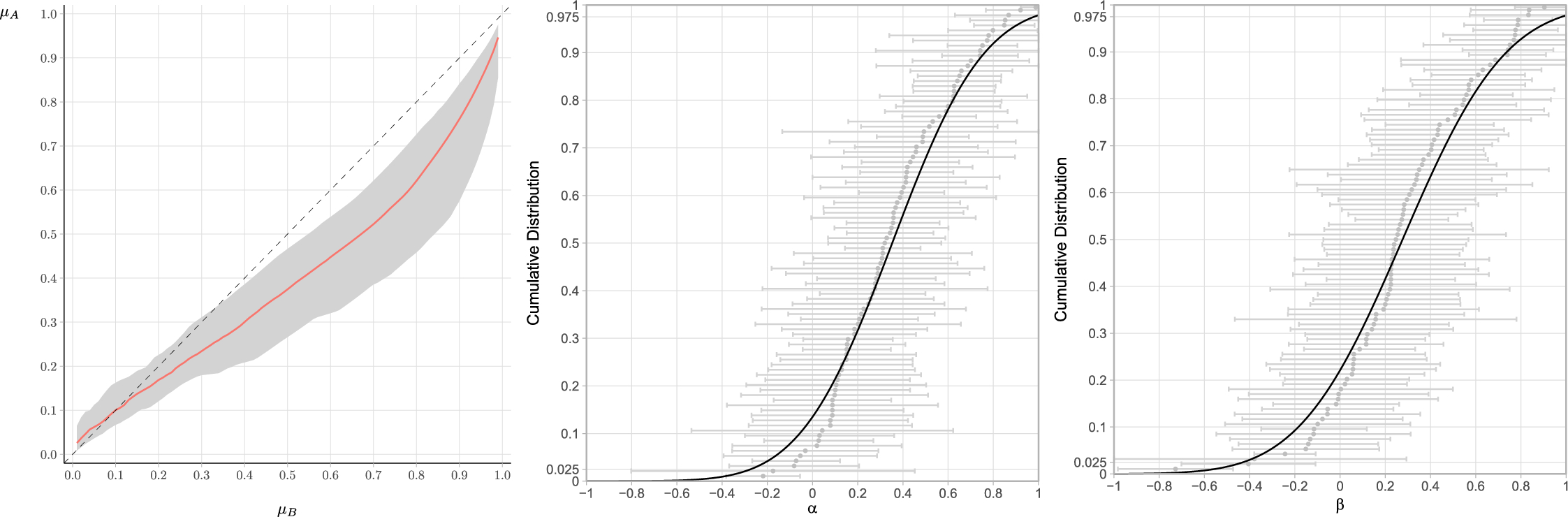
Fig. 4 pmatcher $ϕ_{AB}$ and estimated distributions of its two parameters (Study B)

5.3 Study C

Study C used certainty equivalents to jointly measure beliefs and attitudes toward local (Paris, France, the reference source) versus foreign (Belgrade, Serbia) temperatures.

Our estimations captured a significant mean effect for both the elevation and insensitivity parameters of the function $ϕ_{AB}$ . The average subject exhibited a preference for the local source over the foreign source ( $\bar{β} = 0.059$ , 95% CI $= [0.032; 0.085]$ ). On average, subjects were willing to give up a $\frac{\bar{β}}{2} = 0.03$ winning probability in order to bet on the local source rather than on a 0.5-probability event generated by the foreign source. The average insensitivity parameter indicated slight relative insensitivity ( $\bar{α} = 0.05,$ 95% CI $= [0.012; 0.091]$ ). Subjects were slightly less sensitive to changes in probabilities for the foreign source than for the local one.

We also observed sizable heterogeneity in terms of source dependence for the parameter $β$ (Fig. 5, right panel). For instance, while the average subject exhibited a preference for the local over the foreign source, approximately 30% of the sample exhibited the opposite pattern. Heterogeneity was even larger for the insensitivity parameter $α$ (Fig. 5, middle panel). Around 40% of the sample exhibited a pattern opposite to the average behavior, i.e., these subjects were more sensitive to the foreign source than to the local one.

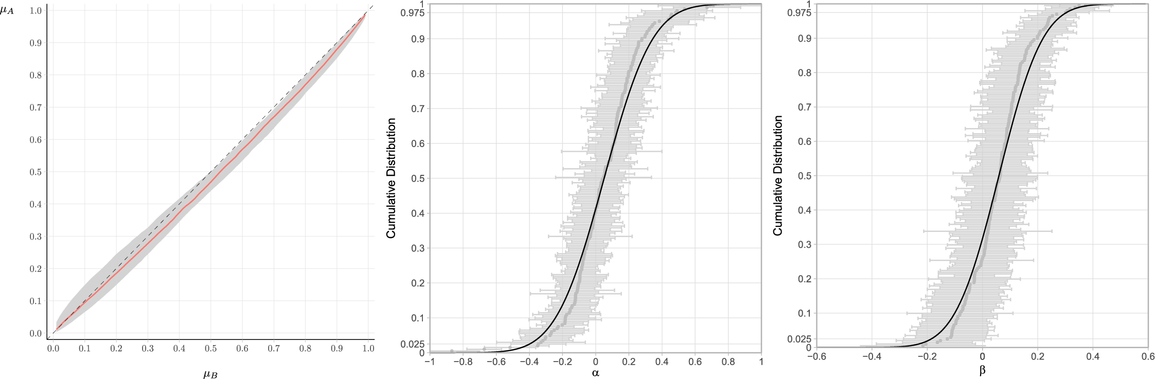
Fig. 5 pmatcher $ϕ_{AB}$ and estimated distributions of its two parameters (Study C)

Study C revealed patterns similar to study B, even though it used different sources, measurement methods (CE vs. MP), and experimental procedures (online with hypothetical choices vs. lab experiment with real incentives). The results showed a consistent preference for the local source, although this was not a universal pattern as some participants exhibited the opposite behavior. Another important finding was that, similar to Study B, the average subject was more insensitive to changes in probability for the foreign source than for the local source, indicating a difference in sensitivity to probability changes between sources.

Comparing the results of this study with those of Study A reinforces the importance of accounting for heterogeneity in attitudes. Although the average magnitude of source dependence was greater in Study C than in Study A, subjects were more likely to exhibit pronounced preferences for one source over the other in Study A. Unlike Study C, which used the same foreign source for all subjects, Study A used different foreign sources for different subjects. This difference in design may explain why we observed more heterogeneity in source dependence in Study A than in Study C.

The main objective of this empirical application is to demonstrate that source dependence and its heterogeneity can be estimated using standard experimental and econometric procedures. Heterogeneity is finely captured by the random-coefficient approach, which focuses on the distribution of parameters in the sample rather than aggregate-level or individual-level parameters. By using Bayesian estimations, we can estimate individual parameters and their precision, which are often overlooked in experimental studies, in addition to the distributions of parameters. We observe that individual-level parameters have large standard errors, which could lead to type II errors if used for inference. This highlights the advantage of random-coefficient estimations, as characteristics of parameter distributions in the sample (such as mean and variance) can be precisely estimated even when the number of observations per subject is too small to derive precise individual estimates. Furthermore, our results reveal a consistent pattern across the three studies: individual standard errors are larger for $β$ than for $α$ . This suggests that relative insensitivity is easier to detect at the individual level than relative optimism.

6 Discussion

6.1 A simple and general method to measure source dependence

Economic decisions often involve choosing between uncertain options with unknown probabilities. These decisions depend not only on the decision maker’s beliefs about uncertain events but also on their attitude toward different sources of uncertainty, a pattern called source dependence. To gain a deeper understanding of such economic decisions, it is crucial to measure source dependence across different situations and individuals.

While existing methods can capture attitudes toward specific sources, there is currently no sound way to convert differences in ambiguity attitudes across sources into source dependence. This paper addresses this limitation and introduces a function $ϕ$ that characterizes source preference between natural sources of uncertainty, independent of risk and ambiguity attitudes. The function maps beliefs about one source of uncertainty to beliefs about another, thereby providing a direct measure of the preference for one source over another. Therefore, it acts as a p(robability) matcher (Baillon et al., Reference Baillon, Bleichrodt, Li and Wakker2023).

We estimated pmatchers on three datasets and showed that source dependence could be efficiently revealed using a limited number of choice-based data using either matching probabilities or certainty equivalents. While using matching probabilities is efficient as it avoids measuring the utility function (Dimmock et al., Reference Dimmock, Kouwenberg and Wakker2016b), it can be challenging for individuals who are not familiar with probabilities (Bouchouicha et al., Reference Bouchouicha, Martinsson, Medhin and Vieider2017). On the other hand, using certainty equivalents is cognitively easier for decision makers but generally requires measuring the utility function (Abdellaoui et al., Reference Abdellaoui, Baillon, Placido and Wakker2011), which increases the number of choices to be collected. Our method provides a simple way to measure source dependence using certainty equivalents without the need to measure utility or weighting functions. As an illustration, we applied our method to a subset of choice tasks from Abdellaoui et al. (Reference Abdellaoui, Baillon, Placido and Wakker2011) and found results that were similar to the original findings in terms of source dependence. Notably, our method required fewer choices than the original study, as it did not rely on the five additional certainty equivalents needed to measure utility.

Our estimation of pmatchers builds on existing methods for separating attitudes from beliefs: the exchangeable-events method (Abdellaoui et al., Reference Abdellaoui, Baillon, Placido and Wakker2011; Baillon, Reference Baillon2008) and the belief-hedging method (Baillon et al., Reference Baillon, Huang, Selim and Wakker2018). While the exchangeable-events method requires a separate task to independently measure beliefs, the belief-hedging method structurally identifies and jointly estimates beliefs and preferences. We extend the belief-hedging approach in three ways. First, our extension of the belief-hedging method provides a direct estimation of source dependence that avoids possible distortions due to the comparison of non-linear ambiguity (or source) functions. Second, it offers an efficient way to quantify source dependence using the belief-hedging method with certainty equivalents without the need to elicit the utility function (Baillon et al., Reference Baillon, Bleichrodt, Keskin, L’Haridon and Li2017). This is well suited for field or online studies (as shown in Study C), as it does not use (matching) probabilities, which may be cognitively difficult for some individuals. However, this approach requires the use of more advanced econometric methods for the joint estimation of beliefs and other parameters. Finally, we use non-linear functions for the structural estimations based on belief-hedging data, whereas previous empirical applications have focused on the neo-additive specification.

6.2 Measuring source dependence beyond two sources

Our method enables the study of source dependence not only between two sources but also among multiple sources. While pmatchers compare attitudes toward two sources, indirect comparisons of source dependence can be made across any two pairs of sources, similar to the role of correlation coefficients when studying several random variables. This is made possible because the source premium is measured on a cardinal scale, making the estimates of different pmatchers comparable. Furthermore, the pmatcher $ϕ$ has properties that facilitate comparisons between more than two sources. The pmatchers between any three sources, A, B, and C, are mathematically related using the composition rule $ϕ_{AC} = ϕ_{AB} \circ ϕ_{BC}$ .Footnote ²¹ Consequently, for three sources, all six possible comparisons can be inferred from only two pmatchers (e.g., $ϕ_{AB}$ and $ϕ_{AC}$ ).

To illustrate, let’s consider the example from Sect. 2 of investors deciding whether to invest in stocks A (AT&T), B (British Telecom), and C (Coca-Cola). These investors are experts in either the telecommunications industry (sources A and B) or the food industry (source C). To study the home bias, one could measure the certainty equivalents of six events for sources A and B using the belief-hedging method to separate attitudes from beliefs. The parameters of the function $ϕ_{AB}$ are directly comparable across individuals and are independent of elements such as risk attitudes, allowing researchers to study whether the home bias is affected by demographic characteristics.

Using the same method, one can measure an additional six certainty equivalents for source C. With our method, it is easy to estimate the function $ϕ_{AC}$ between AT&T and Coca-Cola, capturing a possible effect of expertise on attitudes. The coefficients of the function $ϕ_{AC}$ are not only comparable across individuals but also comparable with those of the function $ϕ_{AB}$ , enabling direct comparison of the effects of home bias and expertise on attitudes.Footnote ²²

6.3 Measuring source dependence without structural econometric estimations

In our empirical illustration of pmatchers, we used structural econometric estimations, which allow accounting for non-deterministic choices (Gaudecker et al., Reference Gaudecker, Wogrolly and Zimpelmann2022). We now show that, under additional assumptions, it is possible to estimate pmatchers without econometrics. Baillon et al. (Reference Baillon, Huang, Selim and Wakker2018) showed that ambiguity attitudes toward a given source could be determined by two indexes, a and b, that can be easily computed using the belief-hedging method without relying on econometrics.Footnote ²³ These indexes are general and can be interpreted under most models of ambiguity attitudes. Under the source model (Abdellaoui et al., Reference Abdellaoui, Baillon, Placido and Wakker2011), the two indexes can be interpreted as the parameters of a neo-additive ambiguity function (e.g., Li et al., Reference Li, Turmunkh and Wakker2019): $f (μ) = c + s μ$ with $s = 1 - a$ and $c = \frac{a - b}{2}$ . Researchers interested in source dependence can thus easily estimate the parameters of neo-additive ambiguity functions toward each source using the matching probabilities of six belief-hedging events for each source, without using econometrics. However, comparing the ambiguity functions of two different sources is not straightforward, as illustrated in Sect. 2.3, and estimation of the pmatcher remains necessary.

The assumption of neo-additivity greatly simplifies the calculation of the pmatcher. Specifically, if $a_{A}, b_{A}, a_{B},$ and $b_{B}$ are the ambiguity parameters of sources A and B, then $ϕ_{AB}$ is also neo-additive with an intercept of $\frac{a_{B} - b_{B} - a_{A} + b_{A}}{2 (1 - a_{A})}$ and a slope of $\frac{1 - a_{B}}{1 - a_{A}}$ . This means that the pmatcher can be easily derived using the indexes of ambiguity attitudes for the two sources. Furthermore, using the reparametrization that we proposed (see Sect. 4.2), we can easily obtain the two parameters of relative insensitivity $α$ and relative optimism $β$ , such that

(8)

\begin{matrix} α = \frac{a_{B} - a_{A}}{1 - a_{A}} and β = \frac{b_{B} - b_{A}}{1 - a_{A}} \end{matrix}

The two parameters of the pmatcher can be computed from the original indexes of the ambiguity functions without requiring any econometric estimations. Furthermore, Eq. 8 holds even if $a_{A}, b_{A}, a_{B},$ and $b_{B}$ are indexes of neo-additive uncertainty functions, which is the case when certainty equivalents are used instead of matching probabilities to assess belief-hedging events. Therefore, our approach, when combined with the assumption of neo-additivity, allows for the estimation of parameters of pmatchers using either matching probabilities or certainty equivalents without requiring any econometrics.

Finally, we note that Eq. 8 illustrates why differences in ambiguity-attitudes parameters may fail to capture source dependence or allow for comparison across sources and individuals. Indeed, the relative optimism parameter $β$ corresponds to the difference in ambiguity aversion parameters between the two sources $b_{B} - b_{A}$ adjusted by the sensitivity toward the “reference source” (role of $1 - a_{A}$ ). This parameter $a_{A}$ , which can vary between individuals and sources, must be accounted for in quantifying source dependence.

6.4 Empirical results: source dependence and its heterogeneity

Our study analyzed pmatchers across three datasets that varied in their elicitation methods and treatment of beliefs. We observed source dependence in all three experiments. In studies B and C, in which the local and foreign sources were identical for all participants, we observed a general preference for local sources over foreign ones, consistent with previous research (Chew et al., Reference Chew, Ebstein and Zhong2012; Fox & Tversky, Reference Fox and Tversky1995). Additionally, we found more relative insensitivity toward foreign sources. These findings parallel previous work on attitudes toward natural sources of uncertainty (Li et al., Reference Li, Müller, Wakker and Wang2017) and suggest that a two-parameter function is necessary to capture the complexity of source dependence.

Studies A and C both used local temperatures and temperatures in a foreign city as sources of uncertainty. However, in Study A, the local source was the same for all participants, while the foreign source differed across participants. In contrast, in Study C, both the local and foreign sources were the same for all participants. This difference in design could explain the difference in empirical patterns between the two studies, particularly the higher heterogeneity in source dependence observed in Study A compared to Study C.

Taking heterogeneity into account refines our understanding of specific economic mechanisms and can generate different predictions from the ones produced by a representative agent (Croitoru & Lu, Reference Croitoru and Lu2014; Cutler et al., Reference Cutler, Finkelstein and McGarry2008). Influential empirical papers have revealed heterogeneity of risk preferences (Bruhin et al., Reference Bruhin, Fehr-Duda and Epper2010; Falk et al., Reference Falk, Becker, Dohmen, Enke, Huffman and Sunde2018; Gaudecker et al., Reference Gaudecker, Van Soest and Wengstrom2011) and ambiguity attitudes within a source of uncertainty, using either Ellsberg urns (Dimmock et al., Reference Dimmock, Kouwenberg, Mitchell and Peijnenburg2016a) or natural sources of uncertainty (Baillon et al., Reference Baillon, Bleichrodt, Keskin, L’Haridon and Li2017; Abdellaoui et al., Reference Abdellaoui, Bleichrodt, Kemel and L’Haridon2021). Our paper contributes to this literature by showing evidence of heterogeneous patterns in terms of source dependence.

Accounting for heterogeneity in source dependence may be as important as accounting for heterogeneity in beliefs or risk attitudes. As Li et al. (Reference Li, Müller, Wakker and Wang2017, p. 1) note, “the domain of nonprobabilized uncertainties is rich just like the domain of non-monetary commodities, with many kinds of informational and emotional configurations.” Source dependence can be explained by different dimensions, including emotions (Li et al., Reference Li, Müller, Wakker and Wang2017), perceived expertise (de Lara Resende & Wu, Reference de Lara Resende and Wu2010), or familiarity (Abdellaoui et al., Reference Abdellaoui, Baillon, Placido and Wakker2011; Chew et al., Reference Chew, Ebstein and Zhong2012). These dimensions can vary widely from one individual to another, leading to high levels of heterogeneity, as seen in Study A (Abdellaoui et al., Reference Abdellaoui, Baillon, Placido and Wakker2011), where foreign cities vary across subjects. Different cities may generate different valence, memories, levels of expertise, or forecast difficulties, for instance. Our method provides a framework for future research to explore how sources’ characteristics interact with individuals’ characteristics and how these interactions affect individuals’ attitudes.

6.5 Applications of source dependence: from individual decisions to strategic interactions

This paper aims to contribute to the growing body of literature in economics that explores the influence of attitudes toward uncertainty on behavior. Initially, this literature focused on the impact of attitudes on individual decision making in various contexts, such as sports events (Heath & Tversky, Reference Heath and Tversky1991; de Lara Resende & Wu, Reference de Lara Resende and Wu2010), elections (Fox & Weber, Reference Fox and Weber2002), stock markets (Kilka & Weber, Reference Kilka and Weber2001; Baillon & Bleichrodt, Reference Baillon and Bleichrodt2015), and insurance markets (Cabantous, Reference Cabantous2007). In recent years, however, researchers have expanded their focus to study the role of uncertainty in strategic interactions.

As Bohnet and Zeckhauser (Reference Bohnet and Zeckhauser2004, p. 474) note, “people care not only about the payoff outcome but also about how the outcome came to be.” Early studies focused on the role of ambiguity aversion in strategic interactions (Calford, Reference Calford2020; Di Mauro & Finocchiaro Castro, Reference Di Mauro and Finocchiaro Castro2011; Kelsey & Le Roux, Reference Kelsey and Le Roux2015; Pulford & Colman, Reference Pulford and Colman2007) and showed that aversion to strategic ambiguity could explain inconsistencies between predictions and behavior in experimental games (Eichberger & Kelsey, Reference Eichberger and Kelsey2011). Recent research has expanded to examine how attitudes toward different sources affect behavior in strategic interactions, i.e., the effect of source dependence in strategic games. For instance, Li et al. (Reference Li, Turmunkh and Wakker2020) showed that integrating source dependence led to a different interpretation of the role of betrayal aversion in the trust game. Other studies have shown that attitudes toward strategic uncertainty depend on the nature of the setting. For instance, Bruttel et al. (Reference Bruttel, Bulutay, Cornand, Heinemann and Zylbersztejn2022) observed that participants were more optimistic in games with strategic complementarity and more pessimistic in games with strategic substitutability. Chark and Chew (Reference Chark and Chew2015) found evidence of ambiguity aversion in competitive games and ambiguity seeking in coordination games. Attitudes in games may also depend on the nature of the opponent; Eichberger et al. (Reference Eichberger, Kelsey and Schipper2008) found that ambiguity-averse behavior was more prevalent when the opponent was a novice, while Kelsey and Le Roux (Reference Kelsey and Le Roux2017) did not find a difference in ambiguity aversion depending on whether the opponent was a local or foreigner.

These findings highlight the importance of source dependence in the context of strategic uncertainty and illustrate that “a failure to incorporate source preference in modeling choice behavior in [strategic interaction settings] will not likely perform well from a descriptive perspective” (Chark & Chew, Reference Chark and Chew2015, p. 222). Existing experimental research on source dependence has mainly relied on comparisons of willingness to bet on different games (Bruttel et al., Reference Bruttel, Bulutay, Cornand, Heinemann and Zylbersztejn2022; Chark & Chew, Reference Chark and Chew2015), the level of uncertainty of chosen actions (Eichberger et al., Reference Eichberger, Kelsey and Schipper2008), or comparisons of ambiguity attitude indexes (Li et al., Reference Li, Turmunkh and Wakker2020). In contrast, our method enables a direct comparison of attitudes toward uncertainty across individuals and games, allowing for a more comprehensive analysis of how attitudes toward different types of contexts, such as competitive versus cooperative, or varying conditions, such as individualized versus unknown opponents, differ based on demographic characteristics like age, gender, or nationality. While previous studies have explored heterogeneity in aversion toward strategic ambiguity (Ivanov, Reference Ivanov2011), investigating heterogeneity in source dependence across individuals and situations in strategic interactions is a promising area for further research.

7 Conclusion

This paper presents a tractable definition of source dependence by introducing a transformation function, that allows for comparisons between individuals and between (pairs of) sources. It further shows how these functions can be estimated from a limited number of choices, adapting commonly used methods to separate attitudes from beliefs. Our empirical analyses of three experimental datasets reveal the presence of source dependence and highlight its heterogeneity across individuals. They further show that source dependence should be studied using two dimensions: relative optimism and relative (in)sensitivity. Our approach provides a framework for future research to examine the determinants of source dependence across individuals and situations.

Supplementary Information

The online version contains supplementary material available at https://doi.org/10.1007/s10683-024-09822-4.

Footnotes

The authors acknowledge financial support from the Investissements d’Avenir Labex Ecodec/ANR-11-LABX-0047 for making this research possible. Note: The replication material for the study is available at https://doi.org/10.3886/E195941V2.

¹ Following (Wakker, Reference Wakker2004), we refer to situations of uncertainty without (with) objective probabilities as ambiguous (risky).

² We define a source of uncertainty as a family of events generated by a similar mechanism of uncertainty (Tversky & Fox, Reference Tversky and Fox1995; Abdellaoui et al., Reference Abdellaoui, Baillon, Placido and Wakker2011).

³ Transformation functions have been used throughout decision theory to capture differences in utility functions (Kreps & Porteus, Reference Kreps and Porteus1978; Klibanoff et al., Reference Klibanoff, Marinacci and Mukerji2005; DeJarnette et al., Reference DeJarnette, Dillenberger, Gottlieb and Ortoleva2020).

⁴ The stimuli proposed by the belief-hedging method can be used to either neutralize the role of beliefs [e.g., (Baillon et al., Reference Baillon, Huang, Selim and Wakker2018)] or to measure beliefs jointly with attitudes [e.g., (Gaudecker et al., Reference Gaudecker, Wogrolly and Zimpelmann2022; Li et al., Reference Li, Turmunkh and Wakker2019)].

⁵ For example, Ellsberg’s two urns example can be accommodated by this model, assuming that probabilistic sophistication holds within each urn.

⁶ Following Dimmock et al. (Reference Dimmock, Kouwenberg and Wakker2016b), we use the notation a-neutral probabilities instead of subjective probabilities. A-neutral probabilities “can be interpreted as the beliefs of the ambiguity neutral twin of the agent” (Baillon et al., Reference Baillon, Bleichrodt, Li and Wakker2021).

⁷ Several authors have proposed considering risk as a specific source of uncertainty. Under this convention, ambiguity aversion ( w a ≠ w ) is a specific case of source dependence: a preference for sources with known probabilities over sources with unknown probabilities.

⁸ Similarly, this investor would require an increase in winning probability of ( μ B - μ A ) in order to bet on source B instead of on source A with a winning event of probability μ A .

⁹ In the present paper, we focus on this relationship, even though Abdellaoui et al. (Reference Abdellaoui, Baillon, Placido and Wakker2011) employed a different approach. They used additional CEs to elicit the utility function and “correct” the function c s for the utility curvature in order to assess the source function w S .

¹⁰ As the data was from a published paper (Abdellaoui et al., Reference Abdellaoui, Baillon, Placido and Wakker2011) we do not have access to the precise payment made to the winning participants.

¹¹ We used the following two information sources for Donald Trump and Emmanuel Macron’s approval ratings: https://elections.huffingtonpost.com and http://www.tns-sofres.com.

¹² In the experiment, we used two periods of time (one month and nine months after the experiment). In this paper, we report only the results obtained for the approval rating one month after the experiment.

¹³ We note that the Prelec and the GE specifications measure the global elevation for different probability levels ( p = 1 / e for the Prelec specification and p = 0.5 for the GE). We propose expressing the global elevation and sensitivity at probability 0.5, which is a natural benchmark for assessing the global shape characteristics.

¹⁴ We note that this reparametrization can also be employed for modeling other functions for which the Prelec or GE specifications are suitable. This is the case, for example, of probability-weighting functions, source functions, ambiguity functions, or even uncertainty functions.

¹⁵ For the descriptive statistics of Study A, see the original paper: Abdellaoui et al. (Reference Abdellaoui, Baillon, Placido and Wakker2011).

¹⁶ In the case of an uncertainty function c S = u - 1 ∘ w S , if u follows a power specification (i.e., u ( x ) = x α ) and the source function w S follows a Prelec specification with parameters δ ′ and γ ′ then c also follows a Prelec with parameters δ = δ ′ / α and γ = γ ′ . In the case of ambiguity function m S = w - 1 ∘ w S , if w and w S both follow a Prelec, then m S also follows a Prelec.

¹⁷ Individual parameters and their standard error are taken respectively as the mean and the standard deviation of individual posterior distributions. The 90% credible interval is computed as the mean more or less 1.64 standard deviations.

¹⁸ In the Bayesian framework, the precision of the estimates is given by their posterior distribution. We thus plot the posterior distribution of the estimates of the mean parameters in the sample.

¹⁹ This is because the mean value β ¯ was almost equal to 0.

²⁰ A consequence of the relative sensitivity is that subjects’ preference for the local source is stronger for low and medium levels of likelihood. This is consistent with Abdellaoui et al. (Reference Abdellaoui, Baillon, Placido and Wakker2011), who found a preference for betting on the temperature in Paris over the temperature in a foreign city for p < 0.5 in the real-incentive subsample.

²¹ This example can be extended to other decompositions. For instance, the pmatcher between B and C can be expressed as ϕ BC = ϕ BA ∘ ϕ AC .

²² We note that the pmatcher ϕ BC between British Telecom and Coca-Cola can be computed without estimation using the composition of the two other pmatchers.

²³ This comes at the cost that no standard error can be computed at the individual level, which prevents assessing the precision of individual-level parameters.

Springer Nature remains neutral with regard to jurisdictional claims in published maps and institutional affiliations.

Springer Nature or its licensor (e.g. a society or other partner) holds exclusive rights to this article under a publishing agreement with the author(s) or other rightsholder(s); author self-archiving of the accepted manuscript version of this article is solely governed by the terms of such publishing agreement and applicable law.

References

Abdellaoui, M., Baillon, A., Placido, L., & Wakker, P. P. (2011). The rich domain of uncertainty: Source functions and their experimental implementation. American Economic Review, 101(2), 695–723. 10.1257/aer.101.2.695CrossRef Google Scholar

Abdellaoui, M., Bleichrodt, H., & Gutierrez, C. (2023). Unpacking overconfident behavior when betting on oneself. Management Science. (Forthcoming).Google Scholar

Abdellaoui, M., Bleichrodt, H., Kemel, E., & L’Haridon, O. (2021). Measuring beliefs under ambiguity. Operations Research, 69(2), 599–612. 10.1287/opre.2020.1980CrossRef Google Scholar

Abdellaoui, M., Kemel, E., Panin, A., & Vieider, F. M. (2019). Measuring time and risk preferences in an integrated framework. Games and Economic Behavior, 115, 459–469. 10.1016/j.geb.2019.03.001CrossRef Google Scholar

Anantanasuwong, K., Kouwenberg, R., Mitchell, O. S., & Peijnenberg, K. (2019). Ambiguity attitudes about investments: Evidence from the field. Working paper. National Bureau of Economic Research, Available at SSRN: https://ssrn.com/abstract=3336513.CrossRef Google Scholar

Armantier, O., & Treich, N. (2013). Eliciting beliefs: Proper scoring rules, incentives, stakes and hedging. European Economic Review, 62, 17–40. 10.1016/j.euroecorev.2013.03.008CrossRef Google Scholar

Attema, A. E., Bleichrodt, H., & L’Haridon, O. (2018). Ambiguity preferences for health. Health Economics, 27(11), 1699–1716. 10.1002/hec.3795CrossRef Google Scholar PubMed

Baillon, A. (2008). Eliciting subjective probabilities through exchangeable events: An advantage and a limitation. Decision Analysis, 5(2), 76–87. 10.1287/deca.1080.0113CrossRef Google Scholar

Baillon, A., & Bleichrodt, H. (2015). Testing ambiguity models through the measurement of probabilities for gains and losses. American Economic Journal: Microeconomics, 7(2), 77–100.Google Scholar

Baillon, A., Bleichrodt, H., Keskin, U., L’Haridon, O., & Li, C. (2017). The effect of learning on ambiguity attitudes. Management Science, 64(5), 2181–2198. 10.1287/mnsc.2016.2700CrossRef Google Scholar

Baillon, A., Bleichrodt, H., Li, C., & Wakker, P. P. (2021). Belief hedges: Measuring ambiguity for all events and all models. Journal of Economic Theory, 198. 10.1016/j.jet.2021.105353CrossRef Google Scholar

Baillon, A., Bleichrodt, H., Li, C., & Wakker, P. P. (2023). Source theory: A tractable and positive ambiguity theory. Working Paper.Google Scholar

Baillon, A., Bleichrodt, H., & Spinu, V. (2020). Searching for the reference point. Management Science, 66(1), 93–112. 10.1287/mnsc.2018.3224CrossRef Google Scholar

Baillon, A., Huang, Z., Selim, A., & Wakker, P. P. (2018). Measuring ambiguity attitudes for all (natural) events. Econometrica, 86(5), 1839–1858. 10.3982/ECTA14370CrossRef Google Scholar

Barham, B. L., Chavas, J-P, Fitz, D., Salas, V. R., & Schechter, L. (2014). The roles of risk and ambiguity in technology adoption. Journal of Economic Behavior & Organization, 97, 204–218. 10.1016/j.jebo.2013.06.014CrossRef Google Scholar

Berger, L., Bleichrodt, H., & Eeckhoudt, L. (2013). Treatment decisions under ambiguity. Journal of Health Economics, 32(3), 559–569. 10.1016/j.jhealeco.2013.02.001CrossRef Google Scholar PubMed

Bohnet, I., & Zeckhauser, R. (2004). Trust, risk and betrayal. Journal of Economic Behavior & Organization, 55(4), 467–484. 10.1016/j.jebo.2003.11.004CrossRef Google Scholar

Bouchouicha, R., Martinsson, P., Medhin, H., & Vieider, F. M. (2017). Stake effects on ambiguity attitudes for gains and losses. Theory and Decision, 83(1), 19–35. 10.1007/s11238-016-9585-5CrossRef Google Scholar

Bruhin, A., Fehr-Duda, H., & Epper, T. (2010). Risk and rationality: Uncovering heterogeneity in probability distortion. Econometrica, 78(4), 1375–1412. 10.3982/ECTA7139Google Scholar

Bruttel, L., Bulutay, M., Cornand, C., Heinemann, F., & Zylbersztejn, A. (2022). Measuring strategic-uncertainty attitudes. Experimental Economics, 26, 1–28.Google Scholar

Cabantous, L. (2007). Ambiguity aversion in the field of insurance: Insurers’ attitude to imprecise and conflicting probability estimates. Theory and Decision, 62(3), 219–240. 10.1007/s11238-006-9015-1CrossRef Google Scholar

Calford, E. M. (2020). Uncertainty aversion in game theory: Experimental evidence. Journal of Economic Behavior & Organization, 176, 720–734. 10.1016/j.jebo.2020.06.011CrossRef Google Scholar

Chark, R., & Chew, S. H. (2015). A neuroimaging study of preference for strategic uncertainty. Journal of Risk and Uncertainty, 50, 209–227. 10.1007/s11166-015-9220-9CrossRef Google Scholar

Chew, S. H., Ebstein, R. P., & Zhong, S. (2012). Ambiguity aversion and familiarity bias: Evidence from behavioral and gene association studies. Journal of Risk and Uncertainty, 44(1), 1–18. 10.1007/s11166-011-9134-0CrossRef Google Scholar

Croitoru, B., & Lu, L. (2014). Asset pricing in a monetary economy with heterogeneous beliefs. Management Science, 61(9), 2203–2219. 10.1287/mnsc.2014.1968CrossRef Google Scholar

Cutler, D. M., Finkelstein, A., & McGarry, K. (2008). Preference heterogeneity and insurance markets: Explaining a puzzle of insurance. American Economic Review, 98(2), 157–62 10.1257/aer.98.2.157CrossRef Google Scholar PubMed

de Lara Resende, J. G., & Wu, G. (2010). Competence effects for choices involving gains and losses. Journal of Risk and Uncertainty, 40(2), 109–132. 10.1007/s11166-010-9089-6CrossRef Google Scholar

DeJarnette, P., Dillenberger, D., Gottlieb, D., & Ortoleva, P. (2020). Time lotteries and stochastic impatience. Econometrica, 88(2), 619–656. 10.3982/ECTA16427CrossRef Google Scholar

Di Mauro, C., & Finocchiaro Castro, M. (2011). Kindness, confusion, or... ambiguity?. Experimental Economics, 14, 611–633. 10.1007/s10683-011-9284-6CrossRef Google Scholar

Dimmock, S. G., Kouwenberg, R., Mitchell, O. S., & Peijnenburg, K. (2016). Ambiguity aversion and household portfolio choice puzzles: Empirical evidence. Journal of Financial Economics, 119(3), 559–577. 10.1016/j.jfineco.2016.01.003CrossRef Google Scholar PubMed

Dimmock, S. G., Kouwenberg, R., & Wakker, P. P. (2016). Ambiguity attitudes in a large representative sample. Management Science, 62(5), 1363–1380. 10.1287/mnsc.2015.2198CrossRef Google Scholar

Easley, D., & O’Hara, M. (2009). Ambiguity and nonparticipation: The role of regulation. The Review of Financial Studies, 22(5), 1817–1843. 10.1093/rfs/hhn100CrossRef Google Scholar

Eichberger, J., & Kelsey, D. (2011). Are the treasures of game theory ambiguous?. Economic Theory, 48(2–3), 313–339. 10.1007/s00199-011-0636-4CrossRef Google Scholar

Eichberger, J., Kelsey, D., & Schipper, B. C. (2008). Granny versus game theorist: Ambiguity in experimental games. Theory and Decision, 64(2–3), 333 10.1007/s11238-007-9053-3CrossRef Google Scholar

Ellsberg, D. (1961). Risk, ambiguity, and the savage axioms. The Quarterly Journal of Economics, 75(4), 643–669. 10.2307/1884324CrossRef Google Scholar

Falk, A., Becker, A., Dohmen, T., Enke, B., Huffman, D., & Sunde, U. (2018). Global evidence on economic preferences. The Quarterly Journal of Economics, 133(4), 1645–1692. 10.1093/qje/qjy013CrossRef Google Scholar

Fox, C. R., & Tversky, A. (1995). Ambiguity aversion and comparative ignorance. The Quarterly Journal of Economics, 110(3), 585–603. 10.2307/2946693CrossRef Google Scholar

Fox, C. R., & Ülkümen, G. (2011). Distinguishing two dimensions of uncertainty. In Brun, , Keren, G., Kirkebøen, G. Montgomery, H. (Eds.), Perspectives on thinking, judging, and decision making (pp. 21–35). Oslo, Norway: Universitetsforlaget.Google Scholar

Fox, C. R., & Weber, M. (2002). Ambiguity aversion, comparative ignorance, and decision context. Organizational Behavior and Human Decision Processes, 88(1), 476–498. 10.1006/obhd.2001.2990CrossRef Google Scholar

Gaudecker, H-M, Van Soest, A., & Wengstrom, E. (2011). Heterogeneity in risky choice behavior in a broad population. American Economic Review, 101(2), 664–94 10.1257/aer.101.2.664Google Scholar

Gaudecker, H.-M., Wogrolly, A., & Zimpelmann, C. (2022). The distribution of ambiguity attitudes. Working Paper.CrossRef Google Scholar

Goldstein, W. M., & Einhorn, H. J. (1987). Expression theory and the preference reversal phenomena. Psychological Review, 94(2), 236 10.1037/0033-295X.94.2.236CrossRef Google Scholar

Heath, C., & Tversky, A. (1991). Preference and belief: Ambiguity and competence in choice under uncertainty. Journal of Risk and Uncertainty, 4(1), 5–28. 10.1007/BF00057884CrossRef Google Scholar

Hoy, M., Peter, R., & Richter, A. (2014). Take-up for genetic tests and ambiguity. Journal of Risk and Uncertainty, 48, 111–133. 10.1007/s11166-014-9186-zCrossRef Google Scholar

Ivanov, A. (2011). Attitudes to ambiguity in one-shot normal-form games: An experimental study. Games and Economic Behavior, 71(2), 366–394. 10.1016/j.geb.2010.05.009CrossRef Google Scholar

Kahneman, D., & Tversky, A. (1979). Prospect theory: An analysis of decision under risk. Econometrica, 47(2), 263–291. 10.2307/1914185CrossRef Google Scholar

Kelsey, D., & Le Roux, S. (2015). An experimental study on the effect of ambiguity in a coordination game. Theory and Decision, 79, 667–688. 10.1007/s11238-015-9483-2CrossRef Google Scholar

Kelsey, D., & Le Roux, S. (2017). Dragon slaying with ambiguity: Theory and experiments. Journal of Public Economic Theory, 19(1), 178–197. 10.1111/jpet.12185CrossRef Google Scholar

Kilka, M., & Weber, M. (2001). What determines the shape of the probability weighting function under uncertainty?. Management Science, 47(12), 1712–1726. 10.1287/mnsc.47.12.1712.10239CrossRef Google Scholar

Klibanoff, P., Marinacci, M., & Mukerji, S. (2005). A smooth model of decision making under ambiguity. Econometrica, 73(6), 1849–1892. 10.1111/j.1468-0262.2005.00640.xCrossRef Google Scholar

Kreps, D. M., & Porteus, E. L. (1978). Temporal resolution of uncertainty and dynamic choice theory. Econometrica, 46(1), 185–200. 10.2307/1913656CrossRef Google Scholar

Lau, S. T., Ng, L., & Zhang, B. (2010). The world price of home bias. Journal of Financial Economics, 97(2), 191–217. 10.1016/j.jfineco.2010.04.002CrossRef Google Scholar

L’Haridon, O., & Vieider, F. M. (2019). All over the map: A worldwide comparison of risk preferences. Quantitative Economics, 10(1), 185–215. 10.3982/QE898CrossRef Google Scholar

Li, C. (2017). Are the poor worse at dealing with ambiguity?. Journal of Risk and Uncertainty, 54(3), 239–268. 10.1007/s11166-017-9262-2CrossRef Google Scholar

Li, C., Turmunkh, U., & Wakker, P. P. (2019). Trust as a decision under ambiguity. Experimental Economics, 22(1), 51–75. 10.1007/s10683-018-9582-3CrossRef Google Scholar

Li, C., Turmunkh, U., & Wakker, P. P. (2020). Social and strategic ambiguity versus betrayal aversion. Games and Economic Behavior, 123, 272–287. 10.1016/j.geb.2020.07.007CrossRef Google Scholar

Li, Z., Müller, J., Wakker, P. P., & Wang, T. V. (2017). The rich domain of ambiguity explored. Management Science, 64(7), 3227–3240. 10.1287/mnsc.2017.2777CrossRef Google Scholar

Millner, A., Dietz, S., & Heal, G. (2013). Scientific ambiguity and climate policy. Environmental & Resource Economics, 55(1), 21 10.1007/s10640-012-9612-0CrossRef Google Scholar

Murphy, R. O., & ten Brincke, R. H. (2017). Hierarchical maximum likelihood parameter estimation for cumulative prospect theory: Improving the reliability of individual risk parameter estimates. Management Science, 64(1), 308–326. 10.1287/mnsc.2016.2591CrossRef Google Scholar

Muthukrishnan, A., Wathieu, L., & Xu, A. J. (2009). Ambiguity aversion and the preference for established brands. Management Science, 55(12), 1933–1941. 10.1287/mnsc.1090.1087CrossRef Google Scholar

Prelec, D. (1998). The probability weighting function. Econometrica, 66(3), 497–527. 10.2307/2998573CrossRef Google Scholar

Pulford, B. D., & Colman, A. M. (2007). Ambiguous games: Evidence for strategic ambiguity aversion. Quarterly Journal of Experimental Psychology, 60(8), 1083–1100. 10.1080/17470210600866354CrossRef Google Scholar PubMed

Savage, L. J. (1954). The foundations of statistics, DoverPress.Google Scholar

Train, K. E. (2009). Discrete choice methods with simulation, Cambridge University Press.Google Scholar

Trautmann, S. T., & van de Kuilen, G. (2015). Ambiguity attitudes. The Wiley Blackwell handbook of judgment and decision making, 1, 89–116. 10.1002/9781118468333.ch3CrossRef Google Scholar

Tversky, A., & Fox, C. R. (1995). Weighing risk and uncertainty. Psychological Review, 102(2), 269 10.1037/0033-295X.102.2.269CrossRef Google Scholar

van de Kuilen, G., & Wakker, P. P. (2011). The midweight method to measure attitudes toward risk and ambiguity. Management Science, 57(3), 582–598. 10.1287/mnsc.1100.1282CrossRef Google Scholar

Viscusi, W. K., & Zeckhauser, R. J. (2015). Regulating ambiguous risks: The less than rational regulation of pharmaceuticals. The Journal of Legal Studies, 44(S2), S387–S422. 10.1086/684305CrossRef Google Scholar

Wakker, P. P. (2004). On the composition of risk preference and belief. Psychological Review, 111(1), 236 10.1037/0033-295X.111.1.236CrossRef Google Scholar