Introduction
Solanum sisymbriifolium L. was introduced in The Netherlands as a trap crop for potato cyst nematodes (PCN) following research that identified the species as the most promising candidate among a diversity of tested potential trap crops (Scholte, Reference Scholte2000a, Reference Scholteb, Reference Scholtec; Scholte and Vos, Reference Scholte and Vos2000). The plant was resistant to PCN (Scholte, Reference Scholte2000a) and showed levels of hatch stimulation between 50 and 80%, i.e. slightly lower than that of potato (Scholte, Reference Scholte2000c; Scholte and Vos, Reference Scholte and Vos2000; Timmermans et al., Reference Timmermans, Vos, Stomph, Van Nieuwburg and Van der Putten2006, Reference Timmermans, Vos, Stomph, Van Nieuwburg and Van der Putten2007b). S. sisymbriifolium originates from South America. Performance of this plant species is being studied for western European field conditions (Timmermans, Reference Timmermans2005, Reference Timmermans, Vos, Van Nieuwburg, Stomph, Van der Putten and Molendijk2007a, Reference Timmermans, Vos, Stomph, Van Nieuwburg and Van der Puttenb). Germination and field emergence are critical processes, as temperatures below 12°C appear to result in slow and irregular emergence (Timmermans et al., Reference Timmermans, Vos, Van Nieuwburg, Stomph, Van der Putten and Molendijk2007a). Therefore, the quantification of the rate and final percentage of emergence is a key element in predicting the potential of the crop in different temperate potato production systems and locations. Early in the season, soil temperatures can be expected to be below 10°C. This is close to the base temperature often observed in crops from warmer ecosystems, e.g. 6–9.5°C for rice (Sié et al., Reference Sié, Dingkuhn, Wopereis and Miezan1998) and 10°C for most maize cultivars (Ruiz et al., Reference Ruiz, Sanchez and Goodman1998). Furthermore, rather high temperature fluctuations can be expected in the top few centimetres of the soil of freshly planted fields. Also, soil moisture conditions close to the surface can be expected to range from near saturated to rather dry, depending on rainfall, radiation and wind.
Under such field conditions, several models have been used to predict rates of developmental processes: the linear thermal time model (e.g. Covell et al., Reference Covell, Ellis, Roberts and Summerfield1986; Steinmaus et al., Reference Steinmaus, Prather and Holt2000; Trudgill et al., Reference Trudgill, Squire and Thompson2000; Alvarado and Bradford, Reference Alvarado and Bradford2002; Jame and Cuttforth, Reference Jame and Cutforth2004), the Q10 model (Watts, Reference Watts1971; Johnson and Thornley, Reference Johnson and Thornley1985) and the bell-shaped beta function (Yin et al., Reference Yin, Kropff, McLaren and Visperas1995; Jame and Cuttforth, Reference Jame and Cutforth2004). The latter can only be fitted when measurements of rates at the supraoptimal range of temperatures are available. This makes the beta model more difficult to validate under typical field conditions. Instead, two new models were tested that have a comparable non-linear behaviour over the lower range of temperatures, i.e. the log-linear or ‘expolinear’ model (Goudriaan and Monteith, Reference Goudriaan and Monteith1990; Lee et al., Reference Lee, Goudriaan and Challa2003) and a quadratic model.
The objectives of the current study were: (1) to assess effects of constant and diurnally fluctuating temperatures and several constant soil moisture levels on the germination and emergence rates of S. sisymbriifolium; (2) to select a temperature response model that accurately predicts the differences in germination and emergence rates of S. sisymbriifolium seeds under controlled conditions, including the temperatures around the base temperature; and (3) to test the model accuracy in prediction of field emergence, measured in independent field experiments.
Materials and methods
Seeds of S. sisymbriifolium were harvested from September to November in 2000, 2001, 2002 and 2003. Red berries were hand picked, washed, crushed and rinsed. Seeds were collected on a sieve and air dried before storage at 12°C and 50% relative humidity.
All data on emergence and germination are expressed as the percentages of the numbers of sown seeds. When germinated on paper (Experiment 2), a seed was considered to have germinated when the root tip was visible. Emergence (all other experiments) was defined as the first visible appearance of plant tissue at the soil surface.
Experiment 1: Effect of different constant temperatures and soil water potential on the rate of emergence
Seeds harvested in 2003 were sown in July 2004 in plastic containers (100 seeds per container) (Greiner Bio-one, Kremsmuenster, Australia) at 1 cm depth, in a mixture of sand (grain size 0.18–1.00 mm) and clay powder (Kaolin, WBB Devon Clays Ltd, Newton Abbot, Devon, UK). The proportion of sand : clay was 6 : 1 on a volume basis, and the pF-curve (soil water retention curve) of the sand–clay mixture was measured to convert volume percentages of water into water potentials. Treatments included five different soil water potentials ranging from c. − 0.96 to − 1.8 × 10− 3 MPa, and five different (constant) temperatures: 9.1°C (standard deviation, SD, 1.7°C), 13.0°C (SD 0.3°C), 16.5°C (SD 0.2°C), 20.0°C (SD 1.0°C) and 21.8°C (SD 0.5°C). Five replicates of 100 seeds were monitored for each of the 25 temperature by soil water potential treatments. Emergence was scored two times each day at the beginning of the experiment, and thereafter the scoring frequency was adapted to the rate of seedling emergence per treatment.
Experiment 2: Effect of fluctuating temperatures on germination
Seeds harvested in 2003 were placed in Petri dishes (100 seeds per dish; dish diameter 9 cm) on two layers of germination paper (filter paper circles, 4.1 g each, diameter 85 mm, product no. 3621, Schleicher & Schuell, Dassel, Germany) moistened with 14 ml of tap water. Petri dishes were placed in an experimental facility consisting of 100 separate, thermally isolated cells (diameter 102 mm, height 33 mm) to each of which an independent temperature regime can be applied using a computerized control system. Thirteen different daily temperature regimes (Fig. 1) were applied in five replicates each. One treatment had a constant temperature of 30°C. Six treatments were defined with mean daily temperatures of 15°C and six treatments with mean daily temperatures of 9°C. Treatments within series differed in maximum amplitude of the daily sine wave, ranging from 0°C (constant temperature) to 10°C. However, in order to prevent chilling or freezing effects, the sine waves in the 9°C series were truncated with minimum temperatures set at 4°C (Fig. 1). Standard deviations of the temperature treatments were < 0.5°C. Germination was scored two times each day at the beginning of the experiment; later, the scoring frequency was adapted to the rate of seed germination per treatment.

Figure 1 Diurnal temperature courses as applied in the 13 different temperature regimes in Experiment 2 for germination tests of Solanum sisymbriifolium seeds. Separate temperature regimes are indicated by numbers in the rest of the manuscript: solid lines represent regime 1, which was a constant 9°C treatment. Regimes 2, 3, 4, 5, 6 were treatments with fluctuating temperatures around 9°C with maximum amplitudes of 2, 4, 6, 8, and 10°C, respectively. Dotted lines represent regime 7, which was a constant 15°C treatment, and regimes 8, 9, 10, 11, 12, which were treatments that fluctuate around 15°C with maximum amplitudes of 2, 4, 6, 8 and 10°C, respectively. The broken line is regime 13, a constant 30°C treatment. Fluctuations were sine functions (of wavelength 1 d) with daily means of 9°C (treatments 2–6) and 15°C (treatments 8–12), respectively. The functions were truncated at 4°C, thus avoiding potential damage due to very low temperatures.
Experiment 3: Field emergence of S. sisymbriifolium seeds
Eleven sowings of S. sisymbriifolium were carried out in the field in the years 2001–2004 on sandy soil near Wageningen (51°58′N, 5°40′E), using a Hege precision-sowing machine (Hege Maschinen, Eging am See, Germany). Sowing depth was 2–4 cm and row distance 12.5 cm. Non-limiting amounts of nutrients were applied. Experiments served more purposes than testing the emergence model (and therefore sowings extended from spring to mid summer) (Timmermans et al., Reference Timmermans, Vos, Van Nieuwburg, Stomph, Van der Putten and Molendijk2007a, Reference Timmermans, Vos, Stomph, Van Nieuwburg and Van der Puttenb).
Temperature was recorded (Datataker DT600, Datataker Data Loggers, Cambridgeshire, UK) during the emergence process at the sowing depth under bare soil using thermocouples (type T, TempControl Industrial Electronic Products, Voorburg, The Netherlands).
In 2001, crops were sown in four replicates at a density of 400 seeds m− 2 on two different dates: first weeks of April and May. In the years 2002 and 2003, crops were sown in four replicates with 200 seeds m− 2 on five dates in total: the first week of May, June and August in 2002, and the third week of June and the first week of August in 2003. In each of the replicate plots sown in 2001–2003, three-row sections of 1 m (with 50 or 25 sown seeds each) were marked with plastic pegs, and within these row sections, emergence counts were made to be able to give an accurate estimate of the time until 50% of the sown seeds had emerged. In 2004, seeds were sown at a density of 200 seeds m− 2 in six replicates on four dates: the fourth week of April, the fourth week of May, the last week of June and the first week of August. In each replicate, two areas of 0.5 × 0.5 m (with 50 sown seeds each) were marked, and emergence counts were made in these areas to monitor the cumulative emergence over time. The average measured soil temperature at sowing depth in the period from sowing to the 50% emergence date was 10.1°C [range: − 0.7 to 29.3°C (absolute minimum and maximum recorded)] for the sowing with the coldest conditions (April 2001) and 32.9°C [range: 16.0–35.8°C (absolute minimum and maximum recorded)] for the sowing under the warmest conditions (August 2003).
Data processing and models
For each temperature treatment in Experiment 1, the progression of cumulative germination with time was fitted to the logistic model y = a+b/(1+e− c ·(x − d)); a, b, c and d being the parameters. With the fitted equation, the time to 50% emergence was calculated (in days). The rate to 50% germination was then calculated as the reciprocal of the time to 50% germination (in d− 1); the same procedure was used to calculate the rate to 50% emergence. Four different models were fitted to these rates to 50% germination or emergence from the different temperature treatments: linear, Q10, expolinear and quadratic models, using Slidewrite Plus for Windows, version 5.01. Further statistics were performed using GenStat 7th edition, version 7.1.0.205.
The widely used ‘linear thermal time model’ starts from fitting a simple linear regression of the rate to 50% germination or emergence (y; units: d− 1) on temperature (T; units: °C) of the form (e.g. Kebreab and Murdoch, Reference Kebreab and Murdoch1999a):
The positive intercept with the T-axis is called the base temperature for germination, T b, below which the rate of development is zero. T b equals –b/a. Hence, equation (1) can be rewritten to become:
which can be rewritten as:
where θ (units: °C d) is the thermal time coefficient, the product of time (1/rate) and the temperature above the base temperature (T b). θ has a constant value for the range of temperatures where the linear model holds.
For the Q10 model (Johnson and Thornly, Reference Johnson and Thornley1985) the rate to 50% germination was fitted as:
in which a, b and c are parameters.
The quadratic model is mathematically equivalent to the ‘square root model’ used to quantify the temperature dependency of biological processes, such as mineralization of organic matter and bacterial growth at suboptimal temperatures (Ratkowsky et al., Reference Ratkowsky, Olley, McMeekin and Ball1982; Bernaerts et al., Reference Bernaerts, Versyck and Van Impe2000). In this model, the rate to 50% germination was fitted as:
in which a, b and c are parameters.
The fourth model we used was the expolinear equation (Goudriaan and Monteith, Reference Goudriaan and Monteith1990; Lee et al., Reference Lee, Goudriaan and Challa2003):
in which a, b and c are parameters.
For all models (1), (4), (5) and (6) the fraction, f t, of completion of the time-accumulated temperature-dependent rate to 50% germination is given by:
where t is time and Δt the increment of time. The cumulative germination is a sigmoid function of the fraction f t and was modelled using the Gompertz equation (Tipton, Reference Tipton1984):
in which g is the cumulative germination and a, b and c are parameters.
The relative performance of the four models was assessed with different criteria, including R 2 of fits and plots of residuals. An additional criterion is derived from rescaling the time axis. If a response model fits perfectly to the data, data points from treatments with constant or daily fluctuating temperatures will fall on one common curve when plotted against f t. For the condition of perfect fit, the point of 50% germination is reached for f t = 1. The linear model is a special case. Here the model also holds if the cumulative germination from different temperature treatments form one single curve when plotted against thermal time, the latter being the product: time × (T − T b). For treatments with fluctuating temperatures, daily increments of f t were obtained from integrating f ts calculated for time steps of 15 min.
Simulations of emergence with the four models were compared with measurements obtained in the field. Simulated time from sowing to 50% emergence was calculated as follows: once each hour, temperatures were measured at sowing depth of each field sowing. These temperatures were used to calculate f t (equation 7) for each hour. With the Gompertz equation (equation 8), the simulated time course of emergence was then calculated, and simulated time to 50% emergence was recorded. Additionally, for each field sowing, the logistic model was fitted through the real data on cumulative emergence over time. All R 2 values of these fits were above 0.92. Using these fits, observed time from sowing to 50% emergence was calculated and plotted against simulated time from sowing to 50% emergence.
Two goodness of fit criteria were used to assess the agreement between model predictions of emergence and observed data, namely the root of the mean square error, RMSE, and the squared bias, SB. The first is defined by:
in which x i is the ith value observed, y i is the ith simulated value and n is the number of data pairs. SB is defined as:
in which x av is the average of all observations and y av is the average of all simulations.
Results
Emergence rates at constant temperatures (Experiment 1)
The time to maximum percentage of emergence from soil at a water potential of − 0.017 MPa increased from 12 d at 21.8°C to 24 d at 16.5°C, to 39 d at 13.0°C and to more than 90 d at 9.1°C. In all temperature treatments, more than 90% of all sown seeds emerged, with exception of the 9.1°C treatment, in which only 68% of the sown seeds emerged (Fig. 2).
Figure 2 Time courses of cumulative seedling emergence of Solanum sisymbriifolium (percentage of sown seeds) in Experiment 1, at a water potential of − 0.017 MPa, for constant temperatures of 21.8°C (◆), 20.0°C (Δ), 16.5°C (▲), 13.0°C (□) and 9.1°C (●).
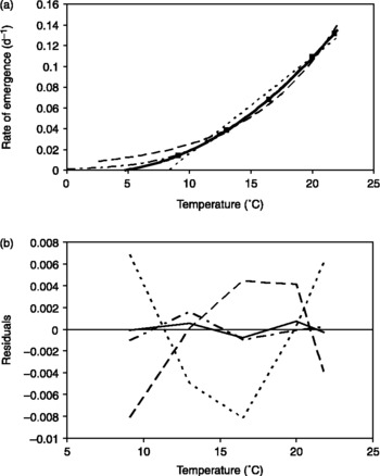
The four temperature response models for germination fitted well to the experimental data of emergence rates (Fig. 3a; Table 1). However, R 2 of the quadratic and the expolinear model were higher than those of the linear thermal time and the Q10 model. The residuals of the quadratic and the expolinear models showed no systematic trend with temperature (Fig. 3b) and were smaller than the residuals of the other models. The residuals of the linear thermal time model and the Q10 models showed parabolic, but opposite relations with treatment temperature (Fig. 3b), indicating inferior fit to the data over the entire range of temperature in comparison with the quadratic and expolinear models.

Figure 3 (a) Rate of emergence (t 50− 1) of Solanum sisymbriifolium seedlings at a water potential of − 0.017 MPa, as a function of treatment temperature in Experiment 1 (■). Standard errors were always smaller than 0.0015 d− 1 and are not shown. Linear (dotted line), Q10 (broken line), expolinear (dot-stripe-dot line) and the quadratic (solid line) models were fitted on rates to 50% emergence. (b) Residuals of the fits of the four models as a function of treatment temperature. The four models are indicated with the same line types as in (a).
Table 1 Overview of the parameter values and their respective standard errors (SE) of the four fitted temperature response models for germination when applied to observed emergence data from Experiment 1

Plots of the observed cumulative emergence versus f (Fig. 4) showed that the seemingly small deviations for data of the linear thermal time and Q10 models in the low temperature range led to large errors in the accuracy of prediction of 50% emergence. If a data series fits perfectly to the model, the cumulative emergence curve passes through the point (θ, 50) for the linear model and (1, 50) for the other three models. For the 9.1°C temperature treatment, the linear thermal time model grossly underestimated and the Q10 model overestimated the progress in emergence. For the linear model, f accumulates faster than is justified in reality, and the curve for 9.1°C in Fig. 4 is shifted to the left of (θ, 50); the opposite is true for the Q10 model.

Figure 4 Cumulative seedling emergence (percentage of sown seeds) of Solanum sisymbriifolium at constant temperatures of 21.8°C (♦), 20.0°C (Δ), 16.5°C (▲), 13.0°C (□) and 9.1°C (●) as function of the linear thermal time (a), and f t calculated with the Q10 model (b), the expolinear model (c) and the quadratic model (d). Lines indicate the point on the x-axis where 50% germination should be reached if the model fit was perfect. This is θ (°C d) for the linear model and a fraction f t = 1 for the other three models.
Germination at fluctuating temperatures (Experiment 2)
In Experiment 2, the point in time of the onset of the steep ‘rise’ of cumulative germination curves occurred at the same value of f t (expolinear model) for all temperature regimes (regardless the magnitude of fluctuation in temperature). This shows that progress in germination was not specifically influenced by temperature fluctuations (Fig. 5) and was completely explained by the daily increment in f t as in constant temperature regimes. Final percentages of germination varied to some extent for temperature regimes 1, 2 and 3 (temperatures of 9°C average and amplitudes of sine-wave fluctuations of 0°C, 2°C and 4°C, respectively.)

Figure 5 Cumulative germination of Solanum sisymbriifolium seeds on filter paper (percentage of sown seeds) for the 13 fluctuating temperature regimes (Experiment 2, indicated by the numbers defined in the legend of Fig. 1) as a function of f t calculated with the expolinear model. Note that in Experiment 2, germination was recorded (versus seedling emergence in Experiments 1 and 3). Germination data do not incorporate time from radicle emergence to seedling emergence.
Effects of soil water potential on emergence (Experiment 1)
The rate of seedling emergence (t 50− 1) at 20°C was not strongly influenced by soil water potential between − 0.21 MPa and − 2.6 × 10− 3 MPa (Fig. 6a). Emergence rate was reduced to practically zero at water potentials of − 0.96 MPa and − 1.8 × 10− 3 MPa, at which almost no seedlings emerged. Final emergence percentages in Experiment 1 had the same trend, being not influenced by soil water potential for water potentials ranging between − 0.21 MPa and − 2.6 × 10− 3 MPa (Fig. 6b), but practically zero at − 0.96 MPa and − 1.8 × 10− 3 MPa.

Figure 6 (a) Rate of seedling emergence of Solanum sisymbriifolium at 20°C as a function of water potential (range: − 0.96 to − 1.8 × 10− 3 MPa) in Experiment 1. (b) Final percentage seedling emergence of sown seeds at 20.0°C as a function of water potential in Experiment 1. Error bars indicate standard errors of the mean.
Comparison of model predictions and observations of field emergence (Experiment 3)
Both indicators for goodness of fit, RMSE and SB, showed little differences (less than 1 d) between the four models when applied to predict field emergence (Table 2). RMSE was highest (1.37 d) for the Q10 model and lowest (0.81 d) for the exponential model. Squared bias (SB) was highest (0.42 d) for the linear model and lowest (0.01 d) for the Q10 model. Figures 7 and 8 show excellent performance of the expolinear model to predict time to 50% emergence (Fig. 7) and the time course of emergence (Fig. 8).
Table 2 Root mean square error, RMSE (equation 9) and squared bias, SB (equation 10) calculated to compare goodness of fit between simulated and observed time of 50% emergence for field sowings in 2001, 2002, 2003 and 2004 (Experiment 3). The sowings with presumed water-potential-influenced emergence rates (open symbols, Fig. 7) were not included

Figure 7 Simulated (using the expolinear model) and observed time from sowing to 50% of seedling emergence from sown seeds of Solanum sisymbriifolium in the field in 2001, 2002, 2003 and 2004 in Experiment 3. Dotted line indicates y = x. The open triangle indicates a data point from a sowing under extremely wet conditions (fields were submerged for several days), and the open square indicates a sowing under extremely hot and dry conditions.

Figure 8 Simulated (using the expolinear model) and observed cumulative emergence curves for the four field sowings of Solanum sisymbriifolium seeds in 2004 (Experiment 3). Model simulations are full-drawn lines; field measurements are individual data points. Sowing dates are shown (Julian day) in the series name. Error bars indicate standard errors of the mean.
Discussion
Especially for the early sowings of S. sisymbriifolium in temperate climates, it can be important to predict emergence rates at temperatures around c. 10°C. Linear thermal time or hydrothermal time models are most commonly used to predict germination rates in various species (e.g. Grundy et al., Reference Grundy, Phelps, Reader and Burston2000; Alvarado and Bradford, Reference Alvarado and Bradford2002; Allen, Reference Allen2003; Larsen et al., Reference Larsen, Bailly, Côme and Corbineau2004). The linear models can be applied only to the range of temperatures for which the data points of rate versus temperature follow a linear relation. As was also pointed out by Hardegree (Reference Hardegree2006), this is a limitation of the linear thermal time model, since data points are bound to deviate from the linear relation near the base end of the response, and near the optimum temperature at the high end of the response. Hardegree (Reference Hardegree2006) suggests that use of other than the linear cardinal-temperature models could be better if the aim is to predict germination rates. Indeed, for S. sisymbriifolium, emergence rates at the base end of its temperature response were systematically underestimated by the linear thermal time model. Quadratic and expolinear models clearly performed better near the ‘base temperature’; virtually all variation in emergence rates of S. sisymbriifolium, associated with temperature treatments in the range of 9.1–21.8°C, could be explained using the quadratic and the expolinear models. Perhaps the expolinear model should be preferred over the quadratic model, as the former behaves linearly at higher temperatures and does not rise quadratically monotonically, which is not in accordance with the generally observed linearity and is conceptually difficult to understand.
The concept of non-linear temperature dependency of rates in plant development is not new (Yin et al., Reference Yin, Kropff, McLaren and Visperas1995; Holshouser et al., Reference Holshouser, Chandler and Wu1996). However, proposed models are often more intricate (beta functions or Weibull functions) and include a decline in rate at temperatures above an optimum temperature. For S. sisymbriifolium, no such decline in germination rate was found for temperatures up to 33°C (unpublished additional results), and the simpler, expolinear model sufficed in describing most of the variations in (field) emergence rates. As temperatures during emergence of over 33°C have little relevance under field conditions in potato-growing areas, further complications seem unnecessary.
Fluctuating temperature regimes were not found to exert specific effects on rate of germination (Fig. 5). Current findings contrast with rate-accelerating effects of fluctuating temperature reported for several other species (Chenopodium album and Panicum maximum, Murdoch et al., Reference Murdoch, Roberts and Goedert1989; Orobanche spp., Kebreab and Murdoch, Reference Kebreab and Murdoch1999b). However, in two of the 11 field sowings, measured emergence rates were substantially lower than the expolinear model predicted (Experiment 3). Weather conditions during the first of these sowings (first week of August, 2002) were very wet; measurements at the nearby Wageningen weather station recorded 37.2 mm of rain immediately after sowing, and as a consequence, two of the four replicate plots were flooded with water for 1 week from the day after sowing onward. In contrast, the late sowing in the first week of August 2003 took place under extremely hot and dry weather conditions. Only 4.8 mm of rain was recorded over the last week of July, and no rain occurred during the first 2 weeks of August in 2003, when the mean diurnal soil temperature at − 5 cm under bare soil was 25.8°C during that period. These extreme wet or dry conditions suggested that emergence rates were probably delayed by high or low water potential, as was also observed in the laboratory (Experiment 1). The fact that such conditions actually occur in field sowings emphasizes the necessity to include moisture effects in a final germination model for S. sisymbriifolium, as has been done for other species, e.g. Solanum tuberosum (Alvarado and Bradford, Reference Alvarado and Bradford2002) and Stellaria media (Grundy et al., Reference Grundy, Phelps, Reader and Burston2000). For the mentioned species, a modification of thermal time on the basis of soil water potential (hydrothermal time) was suggested, but current data are not sufficient to complete this task for S. sisymbriifolium.
The four models were used to predict field emergence data. It should be realized that all models were originally based on emergence data in Experiment 1, and incorporate both germination and post-germination growth of the seedlings to the soil surface. These processes were separated by other authors (Finch-Savage et al., Reference Finch-Savage, Steckel and Phelps1998; Finch-Savage, Reference Finch-Savage, Benech-Arnold and Sánchez2004). It was pointed out that soil penetration resistance is especially important for post-germination seedling growth (Finch-Savage, Reference Finch-Savage, Benech-Arnold and Sánchez2004). By not separating these processes and using the models to predict field emergence, the assumption was made that the penetration resistance of the sandy field soil was the same for all sowings and comparable to that of the sand–clay mixture used in Experiment 1. Part of the deviations in timing between model simulations and field emergence could be caused by these assumptions.
In the application of the four models to predict field emergence date, goodness of fit criteria for models differed only slightly (Table 2), because the field experiments did not include prolonged periods with temperatures around 7–10°C. However, such conditions do occur, especially early in the season, and then predictions with the quadratic or expolinear models would be superior to those obtained with the other models. For S. sisymbriifolium the current expolinear temperature response model of germination rate sufficed to predict temperature effects on field emergence rates (under fluctuating field conditions) without further modifications (Fig. 7). Some unexplained variation in rates of emergence in the field originated presumably from differences in sowing depth and soil compaction. Nevertheless, model predictions of the time from sowing until emergence were so accurate that there is no need for a more complex model for application in agroecological modelling of this species.
It is concluded that the expolinear model is suitable to quantify the temperature dependence of germination and emergence of S. sisymbriifolium in temperate regions. Also, for other crop species that are grown near the low temperature limit of their geographical distribution, including maize, soybean and sunflower, such a simple non-linear model could potentially increase the accuracy of the prediction of emergence rates. In conditions where either too much or too little soil moisture can be expected, a hydro-thermal time model may be needed.
Acknowledgements
The project WEB.5567 was financed by the Technology Foundation STW, Utrecht, The Netherlands. The authors also acknowledge contributions from the Main Board for Arable Products, HPA, The Hague, The Netherlands and from VanDijke Semo, Scheemda, The Netherlands. Thanks are due to members of the STW Users Committee for stimulating discussions.