II. Hedonic Price Theory and Estimation

Rosen (Reference Rosen1974) assumes a good can be characterized by n different attributes z_i whose price is described by a hedonic price function p(z) = p(z ₁, z ₂,…. z_n). The partial derivative of p(z) is termed the marginal implicit price p_i (=∂p(z)/∂z_i). Rosen (Reference Rosen1974) assumes perfect competition and prices p(z) are determined by the market.

Given the market determined p(z), consumers are assumed to choose levels for attributes by maximizing utility (u) subject to an income (y) constraint. This results in a bid (or value) function θ(z; u, y, α), where α specifies individual consumer-specific tastes. The bid function specifies the maximum price they are willing to pay for an attribute z at a fixed level of utility and income given their tastes.

Symmetrically, given p(z), producers are assumed to choose the number of units (M) of the good and levels of z to produce by maximizing profits (π).

(1)$$\eqalignno{& Max\;\pi = M\;p( z ) -C( M, \;\;z_1, \;z_2, \;\ldots z_n ) , \;\cr & \,m, \;z\; } $$

where C(.) represents the total cost function gained after minimizing factor costs given its production technology. It is assumed that C is convex with C_M > 0, $C_{z_i}$> 0, and $C_{z_iz_i}$ > 0.

The first order conditions for maximizing Equation (1) imply:

(2)$$p_i( z ) = C_{z_i}( {M, \;z_1, \;\ldots z_n} ) /M\;\;\;i = 1, \;\ldots n$$

(3)$$p( z ) = C_M( {M, \;\;z_1, \;\ldots .z_n} ) $$

This program results in an offer function ϕ(z; π, β), where β specifies differences among producers in terms of factor prices and technology. The offer function describes the minimum price that producers are willing to receive for attributes z at the fixed level of profit, for the optimally chosen output level. Using Equation (2), profit maximization results in $\phi _{z_i}$ (= ∂ϕ/∂z_i) = $C_{z_i}/M$, that is, the marginal offer function equals the marginal cost per unit of producing the attribute. The optimization program assumes $\phi _{z_i}$ > 0 and $\phi _{z_iz_i}$ > 0.

In equilibrium, tangents among the bid and offer functions “kiss” at various levels of z to trace out p(z). The marginal bid $\theta _{z_i}\;$(= ∂θ/∂z_i), marginal offer $\phi _{z_i}$, and marginal price p_i are equal in equilibrium for attribute z_i. The p(z) function is just a function of z and does not reveal any information about y, α, and β as it is a result of a joint envelope of the bid and offer functions.

To estimate marginal bid and marginal offer functions, a two-stage approach was initially recommended by Rosen (Reference Rosen1974). In the first stage, estimate the hedonic price function in Equation (4):

(4)$$p( z ) = H( {z_{1, }z_{2, } \ldots .z_n} ) $$

and calculate the respective marginal hedonic prices

(5)$$\widehat{{\,p_i}} = \partial \hat{H}( z ) /\partial z_i\;\;\;i = 1, \;2, \;..n.$$

Substitute Equation (5) into the empirical counterpart marginal bid and marginal offer functions:

(6)$$\widehat{{\,p_i}} = F_i( z_1, \;z_2, \;\ldots z_{n, }Y_1)\;\;\;i = 1, \;2, \;..n$$

(7)$$\widehat{{\,p_i}} = G_i( {z_1, \;z_2, \;\ldots z_{n, }Y_2} ) \;\;\;i = 1, \;2, \;..n$$

Equation (6) is the empirical marginal bid function where Y ₁ captures the demand shifters y (income) and α (taste differences). While Equation (7) is the empirical marginal offer (inverse supply) function where Y ₂ captures the supply shifters β (factor price and technology differences).Footnote ¹

Brown and Rosen (Reference Brown and Rosen1982) point out a fundamental identification problem in estimating Equations (6) and (7) from single market data as effectively Equation (4) contains the same information as Equations (6) and (7) unless further restrictions are imposed. At least three methods have been employed to overcome this identification problem: (1) impose restrictions on the functional forms employed (e.g., Quigley, Reference Quigley1982); (2) employ data from multiple markets (Brown and Rosen, Reference Brown and Rosen1982); and (3) use a quasi-experimental setting analyzing markets before and after treatment, event, or shock (Greenstone, Reference Greenstone2017; Banzhaf, Reference Banzhaf2021). For a recent overview of the various approaches, see Taylor (Reference Taylor, Champ, Boyle and Brown2017).

We focus on the use of data from multi-markets for model identification. In this case, Equation (4) is estimated separately for each market, and then using marginal prices from Equation (5), data from all markets are combined to estimate a single marginal bid (Equation (6)) and marginal offer (Equation (7)) function for the individual attributes. Importantly, as articulated by Epple (Reference Epple1987) and subsequently recognized by most studies examining marginal prices, the level of attributes is chosen optimally based on marginal prices and, as such, are endogenous in Equations (6) and (7). This requires the use of techniques such as instrumental variables (IV) to consistently estimate the marginal offer and bid functions.

In terms of identification, as summarized by Ekeland, Heckman, and Nesheim (Reference Ekeland, Heckman and Nesheim2002, p. 309), if there is no variation in consumer preferences or producer technologies across markets, then only one price function exists across markets, and the identification problem arises. However, if preferences and/or technologies differ across markets, then identification is possible. In particular, if consumer preferences do not differ across markets, but technologies do, then the demand function or marginal bid function can be identified. This approach has frequently been employed for housing markets to estimate inverse demand functions, see, for example, Palmquist (Reference Palmquist1984), Bartik (Reference Bartik1987), Zabel and Kiel (Reference Zabel and Kiel2000), Mei, Hite, and Sohngen (Reference Mei, Hite and Sohngen2017), Jun (Reference Jun2019), and Shaw et al. (Reference Shaw, Huang, Lin, Hsu and Tsai2021). In contrast, if consumer preferences differ across markets but producer technologies do not, then the supply function or marginal offer function can be identified.

For the wine market application, we focus on the latter case and the estimation of a marginal offer or inverse supply using a multi-market data approach. Unlike demand studies, it appears only a few studies have explicitly estimated marginal offer functions employing the multi-market data; examples include Witte, Sumka, and Erekson (Reference Witte, Sumka and Erekson1979), Kinzy (Reference Kinzy1982), and Coulson, Dong, and Sing (Reference Coulson, Dong and Sing2021) for housing markets, Pardew, Shane, and Yanagida (Reference Pardew, Shane and Yanagida1986) for agricultural land prices, and Thomas (Reference Thomas1993) for the motor carrier industry. Effectively, the task is to identify separate groups of consumers who have different tastes and preferences for similar goods. If the marginal prices across these separate markets are different, then sufficient data variability will exist to trace out the marginal offer or inverse supply function.

The intuition behind the multiple market approach to supply identification is illustrated in Figure 1, where two separate consumer markets (A and B) exist for the same good. Assume the marginal price function for attribute z_i is downward sloping and exists for two separate markets depicted by the curves $p_{z_i}^A$ and $p_{z_i}^B$. Downward sloping marginal price functions reflect price functions that are increasing at a decreasing rate in attribute levels, which is typical of applications (Taylor, Reference Taylor, Champ, Boyle and Brown2017, p. 239). An upward sloping marginal offer curve is also depicted by the $\phi _{z_i}$ curve. If only one market A existed, the marginal offer curve cannot be identified as only one point (X) on it exists. However, assuming that the model types are similar across the two markets A and B, two points (X and Y) can be identified to trace out the marginal offer curve.Footnote ²

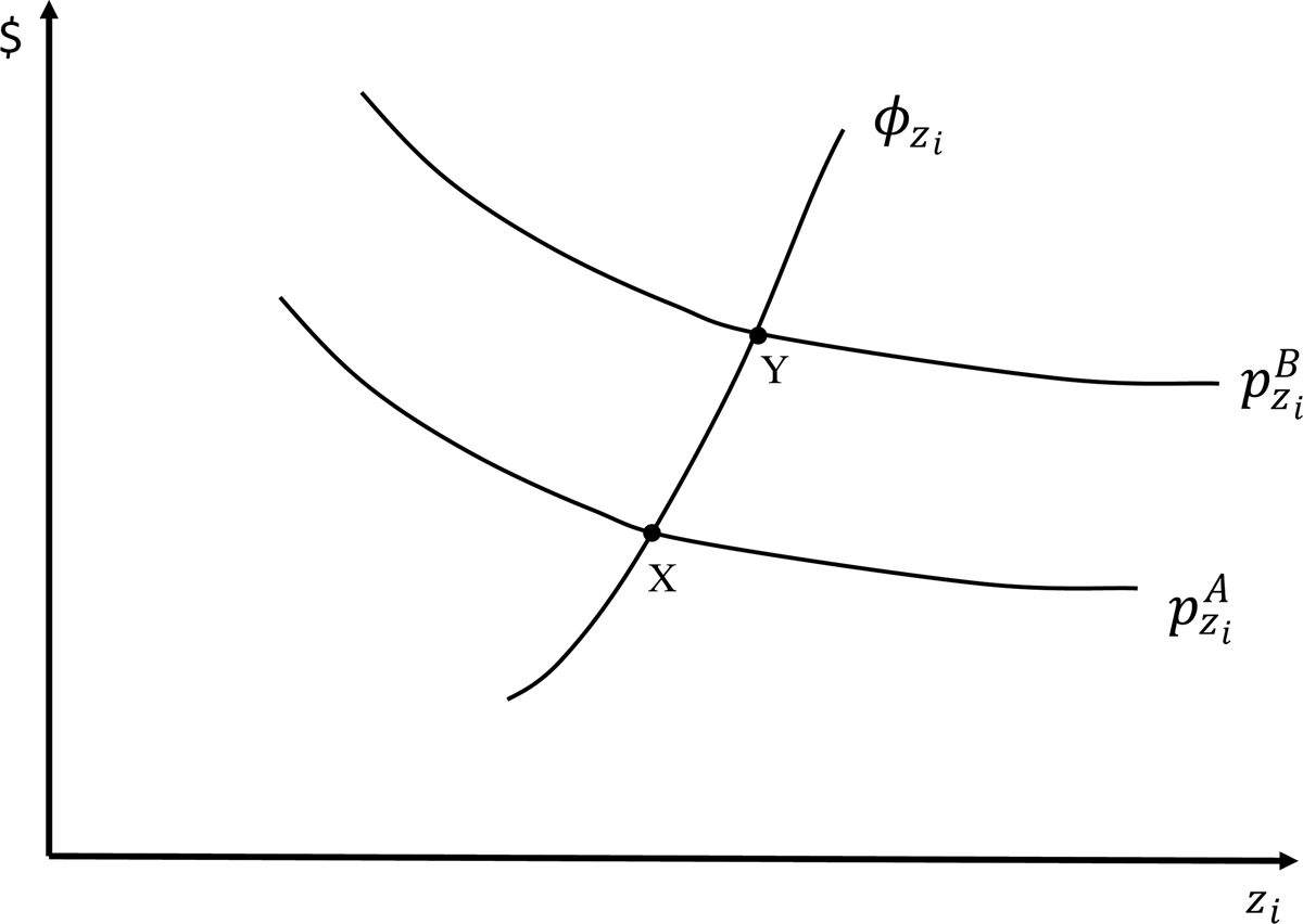
Figure 1 Multi-Market Marginal Offer Function

Given our focus on inverse supply estimation, it is useful to discuss some of the properties of Equation (7). We expect that the own attribute price marginal estimate is positive $\phi _{z_iz_i}$= ∂G_i / ∂z _i > 0, this flows from the convexity assumption of the total cost function and suggests that at the profit maximizing position producers operate on a positively sloped marginal cost curve for the attribute (see, e.g., Palmquist (Reference Palmquist1989, p. 25)). Theoretically, the cross marginal attribute estimates (∂G_i / ∂z _j) are difficult to sign a priori. One possibility is cross attribute effects may also reflect the increased marginal costs of the production of an attribute, as the use of other attributes are increased and hence $\phi _{z_iz_j}$= ∂G_i / ∂z _j > 0. For example, Witte, Sumka, and Erekson (Reference Witte, Sumka and Erekson1979, p. 1168), suggest that their finding that an increase in dwelling size produces an increase in the marginal offer price for dwelling quality simply reflects the greater costs required to produce better dwelling quality as the size of a dwelling increases. Similarly, Thomas (Reference Thomas1993, p. 668) for the motor carrier industry, suggests the estimated higher marginal offer price of service intensity as a result of higher performance, reflects that higher service intensity becomes more costly as performance increases. For non-attribute-related regressors contained in Y ₂, the nature of the supply shifter will determine its impact on marginal offer prices.

It will prove instructive to comment on the role that M (the number of units of the good produced) plays in previously estimated marginal offer functions. The interpretation of estimates for the impact of M on $\phi _{z_i}$ typically relates to a discussion of economies of scale, which may or may not be consistent with the original Rosen (Reference Rosen1974) producer framework. For example, Witte, Sumka, and Erekson (Reference Witte, Sumka and Erekson1979) estimate a negative impact for the number of units owned by a landlord for both dwelling quality and dwelling size marginal prices and suggest this implies economies of scale in the production of houses and quantity discounts. While Thomas (Reference Thomas1993) finds that quantity is largely unimportant and statistically insignificant in various marginal offer models for the motor carrier industry and concludes this implies firms are producing quality in the constant returns of scale range. In general, these interpretations effectively view M as a supply shifter identifying differences among firms in terms of their scale of operation.

III. Hedonic Wine Price Models

In the hedonic wine pricing literature, it appears most studiesFootnote ³ have only estimated the first stage hedonic price function, using Equation (4). Outreville and Le Fur (Reference Outreville and Le Fur2020) provide a classification and summary description of most previously estimated hedonic wine price models and point to a vast array of variables employed in first stage hedonic wine price functions that include weather/climate, soil/terroir, grape region of origin/appellation, grape varieties, public information (including label information and expert ratings), and the wine's age. Outreville and Le Fur (Reference Outreville and Le Fur2020) further classify some studies that suggest the supply of wine impacts price through the use of variables such as producer size or quantity produced in hedonic price functions. An important issue is that some of these previous studies have not made an explicit distinction between z (attributes) and Y ₂ (supply shifters) and have included both variable types in hedonic price functions.

The Rosen (Reference Rosen1974) framework suggests, for a given distribution of consumers (Y ₁) and producers (Y ₂), attributes (z) consist of variables, which influence the utility of consumers and the production costs of producers, in the sense bid and offer functions kiss to determine the market hedonic price function. For example, consider an improvement in a wine's quality (however measured); this will increase a consumer's utility (increasing their bid price) but will also increase the costs of producing the wine for the producer (increasing their offer price). As a consequence, the kiss between bid and offer functions (across Y ₁ and Y ₂) occurs at higher levels of wine quality resulting in a positive marginal price for wine quality. This occurs not because of changes in variation among consumers (Y ₁) and producers (Y ₂) but because of how wine quality enters the typical consumer's utility function and producer's cost function. To this extent, most variables employed in hedonic wine functions can be justified as attributes as they influence the utility and costs of the representative consumer and producer.

If the Rosen framework is adopted, however, the quantity of the wine produced and producer size is producer specific and as such should be excluded from Equation (4) and only employed as Y ₂ in estimating a marginal offer function. Outreville and Le Fur (Reference Outreville and Le Fur2020) list 11 papers that employ the quantity of the wine produced and six studies that employ some measure of producer size in hedonic price functions. In nearly every study, a negative relation between quantity (or producer size) and the price is estimated, and arguments about economies of scale are offered as interpretations.

Several counterarguments, however, have been offered for the inclusion of producer size in Equation (4). For example, Oczkowski (Reference Oczkowski2016a) argues the production from small producers may have some “rarity, scarcity, collectability, exclusivity and cult status” (p. 45) consumer desirable value and hence producer size is included in the price function because it appears in the typical consumer's utility function. Alternatively, the perfect competition assumption is said to be violated, and Rosen's framework is abandoned as some production levels for individual producers are too large, and some aspects of imperfect competition price making occur. Both these arguments are typically not supported by any explicit theoretical development and are offered as ad-hoc justifications for including quantity and producer size in hedonic price functions.

The criticism of the use of producer-specific variables directly in hedonic price functions also applies to the use of producer fixed effects in price models as they control for differences among producers, which are supply shifters rather than attributes. A similar criticism could be made to hedonic price functions where consumer-specific characteristics are included in first-stage models. However, models that employ different consumer characteristics to identify different market segments for wine (Caracciolo and Furno, Reference Caracciolo and Furno2020) may be theoretically justified using a modified Rosen theoretical framework for different market segments (Baudry and Maslianskaia-Pautrel, Reference Baudry and Maslianskaia-Pautrel2016).

IV. Data and the Hedonic Wine Price Function

We consider Australian produced wine sold in different countries as the multi-market data set. Effectively, the same product (Australian wine) is sold in a variety of countries and it is postulated consumers across these countries have different tastes and preferences. In total value terms, Australia is the fourth largest exporter of wines in the world (OIV, 2019). In terms of the total export value of bottled wines, the major export markets Australia serves are China (including Hong Kong and Macau), the United States, and the United Kingdom (Wine Australia, Reference Australia2019a).

The database employed to collect information on the main characteristics of wines is James Halliday's Australian Wine Companion (AWC) (https://www.winecompanion.com.au/). The AWC provides expert quality ratings for approximately 9,000 wines each year. The AWC provides the most authoritative and comprehensive assessment of Australian wines and has been extensively used in hedonic price studies, including Schamel and Anderson (Reference Schamel and Anderson2003) and Oczkowski and Pawsey (Reference Oczkowski and Pawsey2019). Using the AWC as the sampling frame, data on market prices is accessed from wine searcher (https://www.wine-searcher.com/). Average retail market prices were collected for Australian produced wines available for sale during January 2020 from wine merchants located and selling to consumers in four countries: Australia, Hong Kong, the United States, and the United Kingdom.Footnote ⁴ The specific criteria employed for wine sample inclusion is (1) the vintage of the wine is quality rated in the AWC (2020 edition); (2) it is sold by at least three retailers in the country; (3) it is priced less than AUD$500 (to avoid outliers); and (4) it is rated by at least ten Vivino (www.vivino.com) consumer raters (to be employed as an instrument for estimation). To capture the notion of different consumers purchasing similar Australian wines, wines sold in Australia are only included in the analysis if they are available in at least one other country and meet all four sample inclusion criteria. If all wines only sold in Australia were included in the sample, thousands of Australian wines would be part of the sample leading to too many dissimilar wines across countries and the dominance of Australian consumer preferences. The sample of wines is outlined in Table 1. Some noteworthy features include: 48 wines meet all four inclusion criteria for all four countries; the largest wine group occurs with the same 159 wines sold in both Australia and the United Kingdom only. In total, there are 1,297 observations, with most wines sold in Australia (496) and the least in the United States (186).Footnote ⁵

Table 1 Australian Produced Wines Sample: Retailer Locations

Notes: Number of wines sold listed. AUS: Australia; UK: United Kingdom; HK: Hong Kong; US: United States.

For the hedonic price function we employ a standard specification:

(8)$$Price = f( {quality\; rating, \;age\; years, \;wine\; variety, \;wine\; region} ) $$

where Price is the average market retail priceFootnote ⁶ measured in $AUD, all non-Australian prices are converted to $AUD using the average of daily exchange rates for January 2020 (https://rba.gov.au/); Quality Rating is the expert rating score out of 100 from the AWC; Age Years is the difference between 2019 and the year of grape harvest; Wine Variety is a series of dummy variables reflecting the variety employed; and Wine Region is a series of dummy variables reflecting the region from where the grapes are sourced.

The use of expert quality ratings is a dominant feature of many hedonic wine studies. Oczkowski and Doucouliagos (Reference Oczkowski and Doucouliagos2015) have identified more than 40 studies that have employed expert ratings to explain the price. Expert ratings might be viewed as an average measure of consumer preferences (Costanigro, McCluskey, and Goemans, Reference Costanigro, McCluskey and Goemans2010) or as providing opinion leadership for consumers. Both arguments imply that ratings potentially reflect consumer preferences for higher-quality wines. Expert ratings may also capture the higher costs in producing better quality wines, such as the use of better quality grapes or new oak barrels for maturation. Further, in the Australian context, Oczkowski (Reference Oczkowski2016c) demonstrates how expert ratings may also capture the indirect effects of annual weather variations or vintage effects on prices.

Age years capture any consumer preferences for aged wines and the additional costs of maturation and storage for older wines. To control the sample design, we limited the analysis to five major single varieties where at least ten wines are available in each of the four designated countries. The identification of wine regions was based on Australian geographical indications (GIs) and dummy variables defined if at least ten sampled wines in each country existed. For wines not classified to a main region, two variables were employed, wines sourced from a cool climate (long term growing degree days (GDD) less than 1,668) and those from a warm climate (GDD = 1,668 or greater), see Hall and Jones (Reference Hall and Jones2010). Both wine variety and region capture consumer preference and cost of production features for these wine characteristics.Footnote ⁷

Summary sample statistics for the entre sample of wines from all four countries are provided in Table 2. The sample comprises a wide variety of different priced and quality wines. Prices range from less than $9 to more than $350; the mean price of $52 indicates that mainly premium wines dominate the sample. The median price of $39 indicates a highly skewed distribution. Quality scores vary accordingly, from a low of 84 to a high of 99 and an average of 93. The age of wines varies from one to seven years. The most dominant varieties are shiraz (38.5%), chardonnay (20.4%), and cabernet sauvignon (16.9%). The main wine regions are different region cool climate wines (31.2%), Barossa Valley (16.1%), and Margaret River (14%). Wines available in Australia make up (38%) of the sample, the United Kingdom (27%), Hong Kong (20%), and the United States (14%).

Table 2 Summary Statistics

Notes: N = 1,297 covering Australia (496), United Kingdom (355), Hong Kong (260), and United States (186).

The choice of functional form for the hedonic price function has commanded considerable attention in the literature (e.g., Cropper, Deck, and McConnell, Reference Cropper, Deck and McConnell1988). We explicitly consider five commonly employed functions described in Table 3 and choose among them using theoretical and empirical considerations. Rosen (Reference Rosen1974) theoretically questions the use of the linear specification as it implies the possible repacking of a good using different attribute contributions in non-meaningful ways. Further, the linear specification implies a constant marginal price for the attribute. For marginal offer function estimation, this implies marginal prices take on as many values as there are distinct markets, in our case, only four. Rasmussen and Zuehlke (Reference Rasmussen and Zuehlke1990) point to the theoretical limitations of the log-linear specification. For the log-linear specification, marginal attribute prices are just product prices scaled by different constants for each market. This is possibly too restrictive. The other three forms (log-log, quadratic, and log-quadratic) are more theoretically attractive as marginal prices also explicitly depend on attribute levels and can either be increasing or decreasing in attribute levels.

Table 3 Hedonic Functional Forms

Notes: P = price, X ₁ = quality rating, X ₂ = age years. Dummy variables for variety and region only enter as linear terms and each equation contains a constant and error term.

The RESET specification test has been found to usefully discriminate among various linear and log specifications (Godfrey, McAleer, and McKenzie, Reference Godfrey, McAleer and McKenzie1988). RESET tests for the five functional forms and four markets are presented in Table 4. The log-quadratic specification is not rejected for any country, while the log-linear specification is not rejected for two of the four markets. The linear, log-log, and quadratic specifications are all rejected by the RESET test, with the log-log specification being the most strongly rejected. Based on the RESET tests, the log-quadratic form is the preferred specification and is highlighted later with references made to the results from other functional forms.Footnote ⁸

Table 4 Hedonic Price Functions: RESET

Notes: RESET is the robust Ramsey specification error test using the squared predictions and t statistics. ***, **, and * denotes statistically significant at the 1%, 5%, and 10% levels, respectively.

An important issue for the accurate identification of the marginal offer (cost) function is the existence of separate, distinct price functions across markets, as illustrated in Figure 1. Chow tests are presented in Table 5 to examine whether the estimated parameters are statistically the same across the four markets using the log-quadratic form. Pairwise market comparisons indicate that parameters are statistically different among all markets except for the United Kingdom and the United States. Similar results are obtained for the other functional forms. In summary, the Chow tests possibility point to sufficiently significant differences in parameters across markets to justify the multi-market estimation of the marginal offer function.

Table 5 Hedonic Price Functions: Chow-Tests

Notes: Chow Test employs cluster robust (by wine_id) standard errors.

***, **, and * statistically significant at the 1%, 5%, and 10% levels, respectively.