2.1. The structure of the GO system

Figure 1 illustrates the basic structure of a GO system (for Mars rovers), consisting of a matching algorithm with three inputs and one output. First, the dead-reckoned odometry is implemented by CN and WCO to generate the initial trajectory. Second, the gravity measurement (gravity anomaly (adopted by this paper), gravity gradient or deviation of plumb line) of each point is measured by gravimeter or gradiometer. Third, the matching algorithm (Iterative Closest Point (ICP) in this paper) is applied to search the gravity map around the initial trajectory for the optimal gravity sequence. Finally, the position corresponding to the optimal gravity sequence is regarded as the matched trajectory.

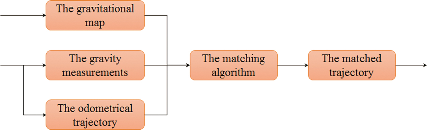
Figure 1. The flowchart of the proposed GO system. The initial trajectory is solved by integrated CN and WCO systems, which is the main PN method for Mars rovers in practical situations. The measurements used in this paper are gravity anomalies.

2.2. Gravity map of Mars

As depicted in Figure 1, the gravitational map itself has influence on the GO system, which has been extensively investigated (Wang et al., Reference Wang, Wang, Fang, Chai and Zheng2012; Reference Wang, Yu, Deng and Fu2016b; Han et al., Reference Han, Wang, Deng, Wang and Fu2017). The attempts to investigate Mars' gravity field started at the end of the 1960s (Ash et al., Reference Ash, Shapiro and Smith1967; Anderson et al., Reference Anderson, Efron and Wong1970). In most cases, the gravitational coefficients are retrieved indirectly from precise spacecraft orbits. The current harmonic coefficients of the models of the Mars gravity field can be achieved to 110 degrees and orders, for example, MRO110B (Konopliv et al., Reference Konopliv, Asmar, Folkner, Karatekin, Nunes, Smrekar and Zuber2011). However, more sophisticated models are needed, while the MRO110B with a spatial resolution of 125 km cannot be used for navigational purposes. Hirt et al. (Reference Hirt, Claessens, Kuhn and Featherstone2012) present a model resolving the resolution down to km-scale, called the Mars Gravity Model 2011 (MGM2011). This model, which combines MRO110B2 with the Mars Orbiter Laser Altimeter (MOLA) topographic model to estimate the short-scale waves (scales of ~3 km to ~125 km), provides surface gravity accelerations and vertical deflections over the entire Martian surface at 3 arcmin resolution. The grid resolution of the map is higher than 2·964 km × 2·964 km (semimajor axis a  =  3,395,428 m).

The statistical properties of the gravity map have a significant influence on the GO system since the core idea of the algorithm is serial correlation (Wang et al., Reference Wang, Zhu, Deng and Fu2016a). Several statistical indices, such as variance, global absolute value of roughness, or slope variance, can be used to evaluate the feature diversity of the gravity map. The indices were used to estimate the topographic features. The absolute value of the roughness of an arbitrary point, however, is the most straightforward and useful property to describe the variations of the gravity feature.

Assuming g(i, j) is the gravity anomaly at a given point (i, j), the roughness R _G of the point is the arithmetic mean value of the roughness in two orthogonal directions R _B and R _L:

(1)$$R_G =(R_B +R_L )/2$$

The subscripts B and L represents the latitude and longitude direction (dimensionless), respectively. The roughness of the two directions is estimated by computing the expected value of the absolute difference of the adjacent points:

(2)$$\eqalign{& R_L = E \vert g(i,j) - g(i,j + 1) \vert \cr & R_B = E \vert g(i,j) - g(i + 1,j) \vert} $$

Figure 2(a) and Figure 3(a) show the 3′ × 3′ (MGM2011) roughness of gravity map of Opportunity and Spirit, respectively. Figure 2(b) and Figure 3(b) are the 0·25′ × 0·25′ (by interpolation) cases. The map roughness around Opportunity is larger than Spirit in most of the image except for some peak values at the edge of the map. Moreover, the traverse points of the rovers are in the middle of the image. The gravity field around the trajectory of Opportunity is rougher.

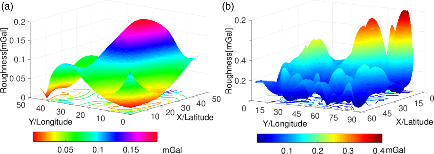
Figure 2. The roughness of gravity map of Opportunity. (a) grid interval 3′ × 3′, (b) 0·25′ × 0·25′. The curve on the underside are roughness isolines of the anomaly. The colour bar represents the roughness value of the map. The X, Y represents latitude and longitude direction (dimensionless), respectively. (a) and (b) are the same area. They have different matrix dimensions.

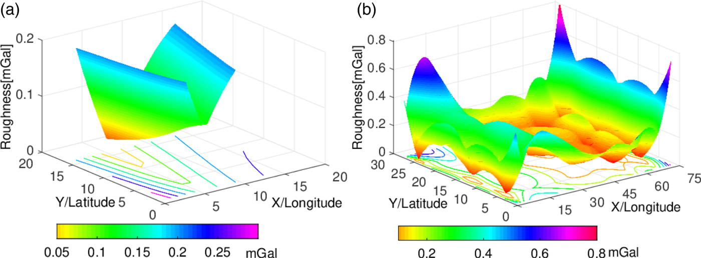
Figure 3. The roughness of gravity map of Spirit. (a) the grid interval is 3′ × 3′, (b) 0·25′ × 0·25′.

2.3. The Matching algorithm

The matching algorithm used in this paper is called Iterative Closest Point (ICP). Besl and McKay (Reference Besl and McKay1992) proposed the algorithm which is based on point-to-point quaternion matching and has been improved many times (Champleboux et al., Reference Champleboux, Lavallee, Szeliski and Brunie1992; Chen and Medioni, Reference Chen and Medioni1991; Zhang, Reference Zhang1994). A high-quality overview of the ICP can be seen in Pomerleau et al., Reference Pomerleau, Colas and Siegwart2015). The idea of the ICP is to find the closest values to the measurements in a background database, which calculates the correlation function of the observations and the matched values iteratively. The relationship between the closest values ${\mathop{p}^{{\rightharpoonup}\prime}}_{ri}$ and the observations ${\mathop{p}^{\rightharpoonup}}_{ri}$ can be transferred by rotation $R({\mathop{q}^{\rightharpoonup}}_R)$ and translation ${\mathop{q}^{\rightharpoonup}}_T$ as:

(3)$${\mathop{p}^{{\rightharpoonup}\prime}}_{ri} = R({\mathop{q}^{\rightharpoonup}}_R){\mathop{p}^{\rightharpoonup}}_{ri} - {\mathop{q}^{\rightharpoonup}}_T$$

The elements of the rotation matrix $R({\mathop{q}^{\rightharpoonup}}_R)$ are the maximum eigenvector of the correlation function matrix aligned by quaternion (Pomerleau et al., Reference Pomerleau, Colas and Siegwart2015). In that way, the difference between ${\mathop{p}^{\rightharpoonup}}_{ri}$ and ${\mathop{p}^{{\rightharpoonup}\prime}}_{ri}$ is

(4)$$\Delta f = \left \vert {\mathop{p}^{{\rightharpoonup}\prime}}_{ri} - {\mathop{p}^{\rightharpoonup}}_{ri} \right \vert $$

The computational process will end if $\Delta f < \tau $ or the iterations are greater than the iterated thresholds. τ is a threshold value.

We use an ICP point-to-point algorithm in this paper for simulation convenience. The method is also adopted partly because the matching process can be completed within several tens of seconds and because the accuracy analysis would be clear and straightforward by using this method. The method can also keep a matched trajectory such as the simulated one.

2.4. The odometrical trajectories

The trajectory data of the twin rovers of MER, Opportunity and Spirit, have been used in this paper (Li et al., Reference Li, Squyres, Arvidson, Archinal, Bell, Cheng and Golombek2005; Matthies et al., Reference Matthies, Maimone, Johnson, Cheng, Willson, Villalpando and Angelova2007). The number of coordinate points for Spirit is 393 and for Opportunity is 1068. The grid resolution (by interpolation) of the maps used in the experiments is 0·25′ × 0·25′ described above for experiments in Sections 3.1 and 3.2. The whole relative trajectories of the rovers are set as one of the inputs. The number of interations is 30 for Sections 3.1 and 3.2 and it is 1000 for Section 3.3. The increase of the iterations is to keep the matched results more stable. The true trajectory is acquired from comprehensive positioning results determined by CN, WCO, and VO (Li et al., Reference Li, Di, Matthies, Folkner, Arvidson and Archinal2004; Reference Li, Squyres, Arvidson, Archinal, Bell, Cheng and Golombek2005; Matthies et al., Reference Matthies, Maimone, Johnson, Cheng, Willson, Villalpando and Angelova2007). The odometrical results of the MER rovers by the above methods are accurate, which can be used as an initial input to the GO system. Therefore, the biases added in Section 3 are assumed to be constant or errors with systematic growth.

3.1. The experiments with different magnitude initial errors

3.1.1. The experimental condition

The initial errors of the MER rovers are about 350 m. These errors will influence the ICP matching process. GO experiments with different magnitude initial errors are introduced in this section. The simulated trajectory is generated by adding biases into the true trajectory:

(5)$$\eqalign{& B_{sim} = B_{real} + \delta B \cr & L_{sim} = L_{real} + \delta L} $$

where the subscript “sim” represents the simulated traverse and “real” is the true trajectory. δ B and δ L are the latitudinal and the longitudinal position biases, respectively. There are six different magnitude errors, which are $\delta B = \delta L = \lsqb 0{\cdot}01^{\circ}\ 0{\cdot}008^{\circ}\ 0{\cdot}006^{\circ}\break 0{\cdot}004^{\circ}\ 0{\cdot}003^{\circ}\ 0{\cdot}002^{\circ}\rsqb $. The distance (on Mars' surface) approximates $\hbox{D}\ = \lsqb 592\, \hbox{m}\, 492\, \hbox{m}\ 392\, \hbox{m}\ 292\, \hbox{m}\ 192\, \hbox{m}\ 92\, \hbox{m}\rsqb$. The threshold value τ to end the ICP process is set as $\tau =2\times 0{\cdot}25^{\prime}$. The accuracy of the gravity anomaly can be up to 0·01 mGal (Lederer, Reference Lederer2009; Creutzfeldt et al., Reference Creutzfeldt, Troch, Guntner, Ferre, Graeff and Merz2014). Considering the differences between the map and measurements, 0·1 mGal random errors are added to the simulated measurements:

(6)$$g_m =g_{real} + rand(\pm 0{\cdot}1)$$

In Equation (7), g _m are the gravity anomaly measurements. g _real is the true value. The “rand” means random function.

3.1.2. Experimental results

3.1.2.1. Experimental result of Mars Spirit

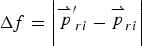
Two results are illustrated in Figure 4. The matching results for Spirit are illustrated in Figures 4(a) and 4(b) in which the initial errors are 600 m and 300 m, respectively. It is shown that the matching trace (green) drifts completely from both the true traverse (red) point and simulated traverse (blue) in Figure 4(a). The matching trace (green) is close to the true trajectory (red) in Figure 4(b). This indicates the GO system has successfully decreased the initial error.

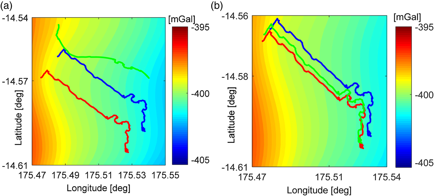
Figure 4. Two matching results between matched trajectory (green) and true trajectory (red) of Spirit when initial bias is about (a) 600 m and (b) 300 m, respectively. The blue trajectory in (a) and (b) means traverse deduced by dead-reckoned odometry. The colour bars represent gravity anomaly value. The meaning of the symbols and colours used here is same as in Figure 6.

The errors between the true trace and the matched trajectory are portrayed in Figures 5(a) and 5(b). The errors illustrated in the two figures show that the GO system has failed when the initial biases are greater than 500 m. The matching process is partially successful when the initial bias is about 400 m. The reason why some parts of the matching trace drift from the true trace is discussed in Section 3.4. The initial bias is significantly decreased when the magnitude of the bias is lower than 300 m. The longitude errors are within 110 m and the latitude errors are within 60 m.

Figure 5. (a) Longitude Error and (b) Latitude Error of the matching traverse in different initial bias (100–600 m) compared with the true trajectory of the Spirit Rover.

3.1.2.2. Experimental results of Mars Opportunity

The true trajectory (red), simulated trajectory (blue), and matched trajectory (green) are illustrated in Figure 6. The initial bias is approximately 600 m in Figure 6(a) and 300 m in Figure 6(b).

Figure 6. Two matching results for Opportunity when initial bias is about (a) 600 m and (b) 300 m, respectively.

As is portrayed in Figures 7(a) and 7(b), the difference between matched position and true trajectory is within 1100 m in longitude and is within 200 m in latitude. When the initial error goes down to around 0·008°, the point before the 1000th point is close to the true position. The difference is reduced by 300 m in longitude when the initial bias is 0·006°. The GO achieves perfect matching when the initial bias equals 0·004°. The difference in both directions remains within 60 metres. When the initial error is reduced to a lower magnitude, the improvement of the positioning result is limited.

Figure 7. (a) Longitude Error and (b) Latitude Error of the matching traverse in different initial bias compared with the true trajectory of the Opportunity Rover.

The absolute positioning results of the initial point (with simulated initial error 400 m) are compared with RT techniques and photographic feature comparison. The results are presented in Table 1. The results acquired by our method are in accordance with the current method. The differences between our method and photographic comparison are small. These results show the method has potential to be an alternative to current absolute-positioning techniques such as RT. The positioning errors of GO can be as large as 1000 m at some points as shown in Figure 7, but the system could be an in-situ, real-time, and autonomous navigational scheme.

Table 1. Absolute positioning results compared with other techniques.

3.2. Experiments with systematic cumulative error of the odometry

The calculated tracks of the rovers will have a large bias from the true trajectory because of the cumulative error caused by the odometry system. In fact, the rovers' calculated track will deviate from its normal path. The WCO and VO techniques cannot eliminate the systematic errors.

3.2.1. The experimental condition

We assume the initial errors have been reduced to within acceptable limits by the GO system described in Section 3.1. That is, the position bias of several points at the beginning between the simulated trajectory and the true trajectory is small. The simulated track is generated as follows:

(7)$$\eqalign{& B_{sim} = B_{real} + N \times 0\cdot 017/3600 \cr & L_{sim} = L_{real} + N \times 0\cdot 017/3600} $$

In Equation (7), the meaning of the subscripts of longitude L and latitude B are the same as in Equation (5). N is the number of points. For Spirit, N = 393 and Opportunity N = 1068. The grid interval of the gravity maps of Mars are 0·25′ × 0·25′. The measurements of gravity anomaly are generated from Equation (6).

3.2.2. Experimental results

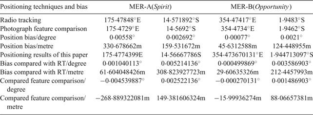
The matched trajectory of Spirit converges to the true track after the 75th point, in which the position biases are within 170 m in two directions. The results are illustrated in Figures 8(a) and 8(b). The matched trajectory (green) portrayed in Figure 8(a) indicates that the matching process is not perfect. The reason is the gravity field around the track is so smooth that the gravity feature cannot be extracted by the ICP algorithm. As portrayed in Figure 9, the matched trajectory of Opportunity converges to the true track quickly, and the position errors are also within 170 m in two directions.

Figure 8. Matching differences between matched trajectory and real (true) trajectory of Spirit with increasing cumulative error (maximum about 110 metres). (a) matching result, and (b) the position errors between the true trajectory and matched trajectory.

Figure 9. Matching differences between matched trajectory and real (true) trajectory of Opportunity with increasing cumulative error (maximum about 300 metres). (a) matching result, and (b) the position errors between the true trajectory and matched trajectory.

3.3. Experiments with other parameters

The relationships between positioning results and the map uncertainty as well as the grid resolution of the map are discussed in this section. The initial errors added to the simulation trajectory equals 400 m.

3.3.1. The uncertainty of the gravity map

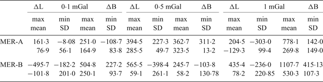
The uncertainty of the gravity map to the positioning results is discussed in term of different magnitude bias (0·1 mGal, 0·5 mGal and 1 mGal) between the map and the real gravity value. The grid resolution is 0·25′ × 0·25′. The positioning errors are shown in Figure 10. The blue line is latitude error and the black line represents longitude error. The ICP algorithm can tolerate a map uncertainty of 1 mGal in the region where the gravity field is coarser, such as in the area around Opportunity. The tolerance is 0·5 mGal in the region around Spirit. Statistical results are shown in Table 2. In most cases, the positioning errors are within 500 m for both Spirit and Opportunity, which suggests the GO could achieve considerable accuracy in practical situations. The mismatch of some points can be adjusted by other suitable algorithms. The ICP or other algorithms should be improved to tolerate larger map uncertainties up to 2–3 mGal. For an underwater case, the level is about 3-5 mGal (Wei et al., Reference Wei, Dong, Liu, Yang, Tang, Gong and Deng2017). The uncertainties are smaller if the measurements are observed in stable circumstances.

Figure 10. The positioning error with respect to different uncertainty of the gravity map. (a) Spirit (b) Opportunity.

Table 2. Statistical results with different gravity uncertainties.

3.3.2. The grid interval of the gravity map

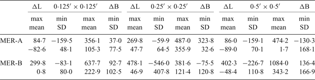
The relationship between the grid resolution and the positioning results is analysed in this section. The errors are illustrated in Figure 11. The grid intervals of the map are 0·125′ × 0·125′, 0·25′ × 0·25′, and 0·5′ × 0·5′. The initial errors added to the simulation trajectory equal 400 m. The measurement uncertainty is 0·1 mGal. The blue line shows errors in latitude and the black one represents the longitude differences. A gravity map with a higher grid interval is needed. A low-resolution map could introduce large positioning errors as shown in Figure 11. The statistical results are shown in Table 3. The improvements of the grid resolution are dependent on the increase of the order and degree of the models. This also needs both satellite and ground-based (on the surface of Mars) measurements. Most of the positioning accuracies are within 500 m.

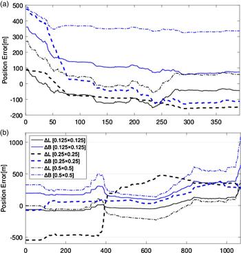
Figure 11. The positioning results with different map spatial resolution. (a) Spirit (b) Opportunity.

Table 3. Statistical results with different background resolution.

The results listed in Table 3 indicate a high grid resolution gravity map is needed because most of the positioning errors correlate with the grid intervals. The grid interval D should be set as small as possible. Table 3 shows that the grid interval of the map is important for the method, in which the lower resolution will mislead the matching process and result in position uncertainties.

3.4. Feasibility analysis

For the two cases, the Gravity-aided Odometry (GO) system can achieve a considerably improved positioning result compared with traditional methods. The system tolerates initial errors with a magnitude up to 500 m where the diversity of the gravity field is larger. The tolerance is about 300 m in a smoother gravity field. The ICP algorithm tolerates map uncertainty up to 1 mGal in the coarser gravity field around the Opportunity regions. A higher accuracy gravity map with lower uncertainty is important to the GO system for rover positioning and autonomous navigation. The GO requires a higher stage-order gravity field to improve both map accuracy and spatial resolution. Moreover, the grid resolution of the map should be as high as possible.

Incorrect matching occurs in the region where the gravity profile lines of the trajectory overlap each other (lines within red rectangle blocks in Figures 12 and 13). This is due to the features of the ICP algorithm. If the profile lines of the different tracks overlap each other in some regions, the matching result will mislead the algorithm, slipping into the wrong position.

Figure 12. The profile line of gravity anomaly of the Spirit trajectory with different magnitude initial error.

Figure 13. The profile line of gravity anomaly of the Opportunity trajectory with different magnitude initial error.

The GO system is highly feasible even though the position bias was large in some cases. The resolution of the map can be improved by new measurements from a Martian orbiter. The uncertainty of the measurements can be limited by using a high accuracy gravity meter or gradiometer and related algorithm. Real-time navigation can be solved by integrating a Kalman Filter with the matching method, as implemented in underwater applications (Wang et al., Reference Wang, Yu, Deng and Fu2016b; Wei et al., Reference Wei, Dong, Liu, Yang, Tang, Gong and Deng2017). The gradient of the gravity could provide more abundant observation information which could improve the positioning accuracy.