


1 Introduction
In this numerical and theoretical study, we examine the oscillatory flow in a swirling fuel injector. We choose this flow for three reasons. First, this flow exhibits self-sustained oscillations, whose control is of both fundamental and industrial interest (Lieuwen Reference Lieuwen2012). Our aim is to identify the wavemaker region of this flow and to devise strategies for its control. The flow is turbulent, so this information would be difficult, if not impossible, to obtain using either nonlinear CFD or stability methods based on equilibrium solutions of the Navier–Stokes equations. Second, we want to examine whether this global stability analysis can handle complex mean flows with several potential instability mechanisms, specifically whether it can identify the primary instability seen in nonlinear direct numerical simulations (DNS). Third, this is the first time to the authors’ knowledge that adjoint-based sensitivity analysis is applied on self-sustained oscillations in an internal turbulent flow.
The chosen flow (figure 1) is from the Datum air swirl fuel injector for a helicopter engine made by Turbomeca. The geometry is axisymmetric. The nozzle consists of an inner non-swirling stream and a coaxial swirling convergent outer flow (Midgley, Spencer & McGuirk Reference Midgley, Spencer and McGuirk2005). Both streams flow from this nozzle into a larger diameter chamber, with an annular outlet downstream. This models the flow in fuel injectors of gas turbine engines. The control of hydrodynamic oscillations in fuel injectors is important for two reasons. First, hydrodynamic oscillations improve mixing of the air/fuel mixture and help to reduce hot spots, which lead to increased nitrous oxide (NOx) formation. Second, hydrodynamic oscillations can couple with acoustic perturbations to enhance or alter thermoacoustic oscillations (Hansford et al. Reference Hansford, OĆonnor, Manoharan and Hemchandra2015; Manoharan et al. Reference Manoharan, Hansford, OĆonnor and Hemchandra2015), which can cause structural damage. At low to moderate Reynolds numbers, similar flows and nozzle geometries are found in the production of carbon nanotubes (Conroy et al. Reference Conroy, Moisala, Cardoso, Windle and Davidson2010).
The time-dependent flow is three-dimensional, while the mean flow is axisymmetric. The mean flow has two large recirculation zones – a conical region around the centreline and an annular region close to the outer wall (the streamlines of the present case will be shown in § 5, figure 4). The inner recirculation zone is formed through an axisymmetric vortex breakdown when the swirl increases in the contracting nozzle, due to conservation of angular momentum (Leibovich Reference Leibovich1978; Syred Reference Syred2006). The outer annular recirculation zone is formed due to confinement. Similar recirculation zones are found in other confined swirling flows, such as swirling pipe flows with sudden expansion (Revuelta Reference Revuelta2004), and confined swirling jet experiments (Billant, Chomaz & Huerre Reference Billant, Chomaz and Huerre1998). The flow in the present injector has been previously studied in the incompressible regime by experiments and large-eddy simulations (LES) (Dunham et al.
Reference Dunham, Spencer, McGuirk and Dianat2008) at relatively high Reynolds numbers (
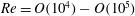 $Re=O(10^{4})-O(10^{5})$
based on the average inflow velocity and radius of the outer nozzle outlet). The observed large-scale oscillations were independent of the Reynolds number within this regime. With zero flow rate in the inner pipe, as in the present study, both LES and experiments showed two peaks in the spectrum. By monitoring the profile at the inlet to the combustion chamber, it was shown that the first peak corresponds to a spiralling mode, and the second peak a double-helical mode.
$Re=O(10^{4})-O(10^{5})$
based on the average inflow velocity and radius of the outer nozzle outlet). The observed large-scale oscillations were independent of the Reynolds number within this regime. With zero flow rate in the inner pipe, as in the present study, both LES and experiments showed two peaks in the spectrum. By monitoring the profile at the inlet to the combustion chamber, it was shown that the first peak corresponds to a spiralling mode, and the second peak a double-helical mode.

Figure 1. Illustration of the flow geometry. A cross-section in the axial–radial plane (constant azimuthal angle), showing the inflow (swirler inlet) and the outflow. The non-dimensional scales are shown: swirler outer diameter (
 $D$
), and the exit velocity from the swirler (
$D$
), and the exit velocity from the swirler (
 $U_{e}$
). The coordinate system is also defined: the origin is at the centreline at the swirler exit location. The relative dimensions of the geometry are the same as in the numerical simulation, except that the numerical domain is longer in the downstream direction.
$U_{e}$
). The coordinate system is also defined: the origin is at the centreline at the swirler exit location. The relative dimensions of the geometry are the same as in the numerical simulation, except that the numerical domain is longer in the downstream direction.
Vortex breakdown, which appears in this injector, is a phenomenon appearing in a wide class of highly swirling flows, with a rotating core and free vortex-like outer region (Leibovich Reference Leibovich1978). Examples are swirling jets and tip vortices around aeroplane wings. When the swirl is increased from zero, the steady axisymmetric breakdown appears as a separation zone near the centreline. With further increases of swirl, typically first the unsteady spiral vortex breakdown (azimuthal wavenumber of unity) appears, and second a succession of other modes with increasing wavenumbers. (In exceptional cases, a spiral vortex breakdown has been reported without axisymmetric breakdown Beran Reference Beran1994.)
A few computations of linear temporal global modes in swirling flows can be found in the literature, and these focus on unconfined vortex breakdown bubbles and swirling jets. The vortex breakdown bubble of the Grabowski vortex (Grabowski & Berger Reference Grabowski and Berger1976) has been studied by DNS (Ruith et al.
Reference Ruith, Chen, Meiburg and Maxworthy2003), by weakly nonlinear analysis (Meliga, Gallaire & Chomaz Reference Meliga, Gallaire and Chomaz2012a
) and by global temporal stability and sensitivity analyses (Gallaire et al.
Reference Gallaire, Ruith, Meiburg, Chomaz and Huerre2006; Qadri, Mistry & Juniper Reference Qadri, Mistry and Juniper2013). The base flow for the Grabowski vortex is axisymmetric and swirling, with a uniform inflow profile for the axial velocity, and a potential vortex for the swirl velocity. After axisymmetric breakdown, one or several recirculation bubbles appear at the centreline. When the swirl or Reynolds number is increased from zero, first a steady recirculation bubble is formed, and second the bubble becomes unstable to a spiralling global mode at a value of the swirl parameter of
 $Sw>0.915$
. The structural sensitivity of the spiralling mode is found to be strongest at the upstream edge of the recirculation bubble (Qadri et al.
Reference Qadri, Mistry and Juniper2013).
$Sw>0.915$
. The structural sensitivity of the spiralling mode is found to be strongest at the upstream edge of the recirculation bubble (Qadri et al.
Reference Qadri, Mistry and Juniper2013).
Global modes in swirling flows have also been successfully studied by local spatio-temporal and spatial stability analyses making the weakly non-parallel flow approximation. In the experiments of Oberleithner, Sieber & Nayeri (Reference Oberleithner, Sieber and Nayeri2011), the swirling jet flow was found to develop self-sustained oscillations when
 $Sw>0.88$
(at a very similar swirl to that of the Grabowski vortex). The frequency and shape of the oscillations was reconstructed through local analysis techniques, in excellent agreement with proper orthogonal decomposition (POD) modes of the experimental data, and more recently the same was done for subcritical (Oberleithner, Paschereit & Wygnanski Reference Oberleithner, Paschereit and Wygnanski2014a
) and forced swirling jets (Oberleithner, Rukes & Soria Reference Oberleithner, Rukes and Soria2014b
). The stability analyses in the above studies were performed around mean flows from experiments. The mean flow stability was observed to produce good results in all regions where the energy production of the eigenmode was positive (i.e. energy was extracted from the mean field), and less good results in the regions where the energy production of the eigenmode was negative (i.e. energy flowing back to the mean field) (Oberleithner et al.
Reference Oberleithner, Rukes and Soria2014b
). Finally, the effect of eddy-viscosity models was considered in Oberleithner et al. (Reference Oberleithner, Stöhr, Im, Arndt and Steinberg2015). While eddy-viscosity models did not change the absolute frequencies, they influenced the absolute growth rates, and by doing this could alter the streamwise location where the global mode frequency was selected. The Newtonian eddy model, as in the present study, was seen to provide the best agreement with experiments regarding both frequency and growth rate.
$Sw>0.88$
(at a very similar swirl to that of the Grabowski vortex). The frequency and shape of the oscillations was reconstructed through local analysis techniques, in excellent agreement with proper orthogonal decomposition (POD) modes of the experimental data, and more recently the same was done for subcritical (Oberleithner, Paschereit & Wygnanski Reference Oberleithner, Paschereit and Wygnanski2014a
) and forced swirling jets (Oberleithner, Rukes & Soria Reference Oberleithner, Rukes and Soria2014b
). The stability analyses in the above studies were performed around mean flows from experiments. The mean flow stability was observed to produce good results in all regions where the energy production of the eigenmode was positive (i.e. energy was extracted from the mean field), and less good results in the regions where the energy production of the eigenmode was negative (i.e. energy flowing back to the mean field) (Oberleithner et al.
Reference Oberleithner, Rukes and Soria2014b
). Finally, the effect of eddy-viscosity models was considered in Oberleithner et al. (Reference Oberleithner, Stöhr, Im, Arndt and Steinberg2015). While eddy-viscosity models did not change the absolute frequencies, they influenced the absolute growth rates, and by doing this could alter the streamwise location where the global mode frequency was selected. The Newtonian eddy model, as in the present study, was seen to provide the best agreement with experiments regarding both frequency and growth rate.
In the present study, we have chosen to perform a global mode analysis around a mean flow, instead of an equilibrium solution to the Navier–Stokes equations. Equilibrium solutions are very difficult to obtain for this flow at Reynolds numbers above
 $Re=250$
, due to axisymmetric convective shear layer instabilities, which appear as soon as the flow exits the nozzle. At higher Reynolds numbers, the convective instabilities develop into turbulence before the mean flow reaches the exit of the domain, and before the self-sustained oscillation (global instability) dominates.
$Re=250$
, due to axisymmetric convective shear layer instabilities, which appear as soon as the flow exits the nozzle. At higher Reynolds numbers, the convective instabilities develop into turbulence before the mean flow reaches the exit of the domain, and before the self-sustained oscillation (global instability) dominates.
Stability analysis around a turbulent mean flow is controversial but has been widely discussed, particularly in the reduced-order modelling community. The mean-field theory introduced by Noack et al. (Reference Noack, Afanasiev, Morzynski, Tadmor and Thiele2003) states that a stability analysis around a mean flow will produce the limit cycle as a neutrally stable global mode, which was later confirmed by Barkley (Reference Barkley2006) for the cylinder flow. The result for the cylinder flow is not universal; criteria for its validity and the effect of nonlinear harmonics has been discussed, for example, by Sipp & Lebedev (Reference Sipp and Lebedev2007) and Mezic (Reference Mezic2013). The need to include turbulent dissipation (eddy-viscosity) models in reduced-order models, independently of harmonics, has been discussed, for example, by Luchtenburg et al. (Reference Luchtenburg, Günther, Noack, King and Tadmor2009), Östh et al. (Reference Östh, Noack, Krajnovic, Barros and Bore2014) and Protas, Noack & Östh (Reference Protas, Noack and Östh2015). Mean flow stability has been used for many studies of convective instability (including the seminal works of Gaster, Kit & Wygnanski Reference Gaster, Kit and Wygnanski1985; Cohen & Wygnanski Reference Cohen and Wygnanski1987; Weisbrot & Wygnanski Reference Weisbrot and Wygnanski1988) and transient growth (Hoyas & Jimenez Reference Hoyas and Jimenez2006; Pujals et al. Reference Pujals, Garcia-Villalba, Cossu and Depardon2009). Here, we will focus on the oscillator behaviour and, in particular, its adjoint-based sensitivity.
After Barkley (Reference Barkley2006), global mode analysis has been applied to identify large-scale structures in turbulent flows in a number of studies, and these can be can be divided into three categories following Mettot, Sipp & Bézard (Reference Mettot, Sipp and Bézard2014b ). In the quasi-laminar approach, the Navier–Stokes equations, using molecular viscosity for the viscous term, are linearized around the mean flow derived from nonlinear simulations. In the base flow approach, a turbulence model equation such as URANS is considered, and the equation and the turbulence model are both linearized around a fixed point of the model. A special case in between the two is a frozen eddy viscosity approach, where a turbulent eddy viscosity is determined from nonlinear data, and applied as a spatially varying viscosity in the stability analysis, while the turbulent Reynolds stresses themselves are not linearized.
Here, we are especially interested in the sensitivity of the eigenvalue to changes in the system. Several sensitivity studies of turbulent flows have been performed recently. The base flow approach was used by, for example, Meliga, Pujals & Serre (Reference Meliga, Pujals and Serre2012b
) to compute the sensitivity of a turbulent (
 $Re=13\,000$
) flow around a D-shaped bluff body, using URANS equations combined with a linearized Spalart–Allmaras model. The most sensitive region for passive control was successfully matched against experiments. Other successful studies include Mettot, Renac & Sipp (Reference Mettot, Renac and Sipp2014a
) and Crouch, Garbaruk & Magidov (Reference Crouch, Garbaruk and Magidov2007). The base flow approach is mathematically fully consistent. However, an accurate representation of the physics requires a model which can reproduce both the mean flow and the perturbation field accurately. For swirling flows, URANS models generally struggle to predict the mean flow swirl profile accurately (Wallin & Johansson Reference Wallin and Johansson2000; Dunham et al.
Reference Dunham, Spencer, McGuirk and Dianat2008), whereas the mean swirl profile is crucial for vortex breakdown instabilities as seen above. Hence, we need to adopt an approach which ensures correct mean flow scales. Algebraic Reynolds stress models might be appropriate (Wallin & Johansson Reference Wallin and Johansson2000), but are very complicated to linearize even in one dimension (Gupta Reference Gupta2014), while our mean flow is two-dimensional.
$Re=13\,000$
) flow around a D-shaped bluff body, using URANS equations combined with a linearized Spalart–Allmaras model. The most sensitive region for passive control was successfully matched against experiments. Other successful studies include Mettot, Renac & Sipp (Reference Mettot, Renac and Sipp2014a
) and Crouch, Garbaruk & Magidov (Reference Crouch, Garbaruk and Magidov2007). The base flow approach is mathematically fully consistent. However, an accurate representation of the physics requires a model which can reproduce both the mean flow and the perturbation field accurately. For swirling flows, URANS models generally struggle to predict the mean flow swirl profile accurately (Wallin & Johansson Reference Wallin and Johansson2000; Dunham et al.
Reference Dunham, Spencer, McGuirk and Dianat2008), whereas the mean swirl profile is crucial for vortex breakdown instabilities as seen above. Hence, we need to adopt an approach which ensures correct mean flow scales. Algebraic Reynolds stress models might be appropriate (Wallin & Johansson Reference Wallin and Johansson2000), but are very complicated to linearize even in one dimension (Gupta Reference Gupta2014), while our mean flow is two-dimensional.
The frozen eddy viscosity performed almost as well as the fully linearized turbulent viscosity for a cavity flow (Crouch et al. Reference Crouch, Garbaruk and Magidov2007). It has also performed well in swirling flow studies using local spatio-temporal techniques in injector flows (Oberleithner et al. Reference Oberleithner, Stöhr, Im, Arndt and Steinberg2015). Finally, Camarri, Fallenius & Fransson (Reference Camarri, Fallenius and Fransson2013) obtained a good agreement with the experimental structural sensitivity region for a porous cylinder flow using only molecular viscosity (the quasi-laminar approach), and similarly Mettot et al. (Reference Mettot, Sipp and Bézard2014b ) for a D-shaped cylinder.
In the present study, we start by characterizing the nonlinear dynamics of the swirl injector in DNS, and extracting the dominant mode shapes and frequencies by POD. We then construct a Newtonian eddy-viscosity model (Reynolds & Hussain Reference Reynolds and Hussain1972) from nonlinear simulation data in the manner suggested but not implemented in Mettot et al. (Reference Mettot, Sipp and Bézard2014b ), and apply this in the global mode and sensitivity computation in the form of a frozen eddy viscosity. We investigate the instability mechanism for the dominant spiralling mode in terms of the location of the structural sensitivity and the relative magnitudes of structural sensitivity tensor components. Finally, we discuss the observed similarities and differences between the results with frozen eddy viscosity and molecular viscosity, and between this flow and the D-shaped cylinder.
2 Interpretation of stability analysis around a turbulent mean flow
Mathematical interpretation of the stability analysis around the mean flow is not as straightforward as the stability analysis around a steady solution of the Navier–Stokes equations. Nevertheless, a qualitative mathematical and physical interpretation of mean flow stability results and qualitative criteria for their validity can be found. The argument below follows the main lines presented in Turton, Tuckerman & Barkley (Reference Turton, Tuckerman and Barkley2015). In the present study, a triple decomposition of the flow field is introduced following Reynolds & Hussain (Reference Reynolds and Hussain1972):
 $$\begin{eqnarray}\boldsymbol{u}=\overline{\boldsymbol{u}}+\widetilde{\boldsymbol{u}}+\boldsymbol{u}^{\prime },\end{eqnarray}$$
where
 $\overline{\phantom{u}}$
is the time-average operator,
$\overline{\phantom{u}}$
is the time-average operator,
 $(\,\widetilde{\phantom{u}}+\overline{\phantom{u}})$
is the phase-average operator, and
$(\,\widetilde{\phantom{u}}+\overline{\phantom{u}})$
is the phase-average operator, and
 $\boldsymbol{u}^{\prime }=\boldsymbol{u}-\overline{\boldsymbol{u}}-\widetilde{\boldsymbol{u}}$
is the fluctuation with zero phase average. The three terms are the mean flow (
$\boldsymbol{u}^{\prime }=\boldsymbol{u}-\overline{\boldsymbol{u}}-\widetilde{\boldsymbol{u}}$
is the fluctuation with zero phase average. The three terms are the mean flow (
 $\overline{\boldsymbol{u}}$
), the organized wave containing all coherent time-periodic large-scale motions (
$\overline{\boldsymbol{u}}$
), the organized wave containing all coherent time-periodic large-scale motions (
 $\widetilde{\boldsymbol{u}}$
), and the stochastic part containing the remaining incoherent turbulent motions (
$\widetilde{\boldsymbol{u}}$
), and the stochastic part containing the remaining incoherent turbulent motions (
 $\boldsymbol{u}^{\prime }$
). The equation for the mean flow is obtained by taking the time average of the Navier–Stokes equations:
$\boldsymbol{u}^{\prime }$
). The equation for the mean flow is obtained by taking the time average of the Navier–Stokes equations:
 $$\begin{eqnarray}\overline{\boldsymbol{U}}\boldsymbol{\cdot }\boldsymbol{{\rm\nabla}}\overline{\boldsymbol{U}}=-\boldsymbol{{\rm\nabla}}\overline{P}+\boldsymbol{{\rm\nabla}}\boldsymbol{\cdot }(Re^{-1}\overline{\unicode[STIX]{x1D64E}}-\overline{\widetilde{\boldsymbol{u}}\widetilde{\boldsymbol{u}}}-\overline{\boldsymbol{u}^{\prime }\boldsymbol{u}^{\prime }}),\end{eqnarray}$$
while the organized wave satisfies the phase-averaged Navier–Stokes equations, with (2.2) subtracted:
 $$\begin{eqnarray}\frac{\partial \widetilde{\boldsymbol{u}}}{\partial t}+\overline{\boldsymbol{U}}\boldsymbol{\cdot }\boldsymbol{{\rm\nabla}}\widetilde{\boldsymbol{u}}+\widetilde{\boldsymbol{u}}\boldsymbol{\cdot }\boldsymbol{{\rm\nabla}}\overline{\boldsymbol{U}}=-\boldsymbol{{\rm\nabla}}\widetilde{p}+\boldsymbol{{\rm\nabla}}\boldsymbol{\cdot }(Re^{-1}\widetilde{\unicode[STIX]{x1D668}}-\widetilde{\widetilde{\boldsymbol{u}}\widetilde{\boldsymbol{u}}}-\widetilde{\boldsymbol{u}^{\prime }\boldsymbol{u}^{\prime }}).\end{eqnarray}$$
In the above,
 $\unicode[STIX]{x1D64E}=\boldsymbol{{\rm\nabla}}\boldsymbol{U}+\boldsymbol{{\rm\nabla}}\boldsymbol{U}^{\text{T}}$
is the mean flow shear stress tensor, and
$\unicode[STIX]{x1D64E}=\boldsymbol{{\rm\nabla}}\boldsymbol{U}+\boldsymbol{{\rm\nabla}}\boldsymbol{U}^{\text{T}}$
is the mean flow shear stress tensor, and
 $\widetilde{\unicode[STIX]{x1D668}}$
the stress tensor of the organized wave. We will proceed by assuming that the coherent motions consist of discrete fundamental limit cycles and their harmonics, and can hence be Fourier-decomposed as:
$\widetilde{\unicode[STIX]{x1D668}}$
the stress tensor of the organized wave. We will proceed by assuming that the coherent motions consist of discrete fundamental limit cycles and their harmonics, and can hence be Fourier-decomposed as:
 $\widetilde{\boldsymbol{u}}\approx \sum _{m>0}\sum _{n\neq 0}\boldsymbol{u}_{m,n}\exp (\text{i}n{\it\omega}_{m}t)$
.
$\widetilde{\boldsymbol{u}}\approx \sum _{m>0}\sum _{n\neq 0}\boldsymbol{u}_{m,n}\exp (\text{i}n{\it\omega}_{m}t)$
.
For simplicity, let us first consider the case where limit cycles with different
 $m$
, and their products, are harmonically unrelated to each other (at the end of the section, we will return to the case where they are harmonically related). When substituting the Fourier decomposition of the coherent part into (2.2), we obtain:
$m$
, and their products, are harmonically unrelated to each other (at the end of the section, we will return to the case where they are harmonically related). When substituting the Fourier decomposition of the coherent part into (2.2), we obtain:
 $$\begin{eqnarray}\overline{\boldsymbol{U}}\boldsymbol{\cdot }\boldsymbol{{\rm\nabla}}\overline{\boldsymbol{U}}=-\boldsymbol{{\rm\nabla}}\overline{P}+\boldsymbol{{\rm\nabla}}\boldsymbol{\cdot }\left(Re^{-1}\overline{\unicode[STIX]{x1D64E}}-\mathop{\sum }_{m>0}\mathop{\sum }_{n>0}\boldsymbol{u}_{m,n}\boldsymbol{u}_{m,-n}-\overline{\boldsymbol{u}^{\prime }\boldsymbol{u}^{\prime }}\right).\end{eqnarray}$$
This shows that the mean flow is influenced by the coherent motions, through the interaction of each fundamental mode with its conjugate, and the interaction of each harmonic with its conjugate. The mean flow is also influenced by the Reynolds stresses arising from the incoherent motions.
Similarly, when substituting the Fourier decomposition into (2.3), we obtain for
 $n=1$
(the limit cycle fundamental):
$n=1$
(the limit cycle fundamental):
 $$\begin{eqnarray}-\text{i}{\it\omega}\boldsymbol{u}_{m,1}+\overline{\boldsymbol{U}}\boldsymbol{\cdot }\boldsymbol{{\rm\nabla}}\boldsymbol{u}_{m,1}+\boldsymbol{u}_{m,1}\boldsymbol{\cdot }\boldsymbol{{\rm\nabla}}\overline{\boldsymbol{U}}=-\boldsymbol{{\rm\nabla}}p_{m,1}+\boldsymbol{{\rm\nabla}}\boldsymbol{\cdot }\left(\!Re^{-1}\unicode[STIX]{x1D64E}_{m,1}-\!\mathop{\sum }_{n\neq 0,1}\!\boldsymbol{u}_{m,n}\boldsymbol{u}_{m,1-n}-(\widetilde{\boldsymbol{u}^{\prime }\boldsymbol{u}^{\prime }})_{m}\!\right)\!.\end{eqnarray}$$
Hence, the limit cycle
 $m$
may be influenced by the coherent motions, through the interaction of the first harmonic
$m$
may be influenced by the coherent motions, through the interaction of the first harmonic
 $\boldsymbol{u}_{m,2}$
with the conjugate of the fundamental
$\boldsymbol{u}_{m,2}$
with the conjugate of the fundamental
 $\boldsymbol{u}_{m,-1}$
, and the interaction of each higher harmonic with the conjugate of its preceding harmonic. It may also be influenced by
$\boldsymbol{u}_{m,-1}$
, and the interaction of each higher harmonic with the conjugate of its preceding harmonic. It may also be influenced by
 $(\widetilde{\boldsymbol{u}^{\prime }\boldsymbol{u}^{\prime }})_{m}$
, which is the oscillation of the incoherent Reynolds stresses at frequency
$(\widetilde{\boldsymbol{u}^{\prime }\boldsymbol{u}^{\prime }})_{m}$
, which is the oscillation of the incoherent Reynolds stresses at frequency
 ${\it\omega}={\it\omega}_{m}$
.
${\it\omega}={\it\omega}_{m}$
.
Let us now introduce the linearized Navier–Stokes operator, where the linearization is performed around the mean flow, acting on any velocity field
 $\boldsymbol{u}$
:
$\boldsymbol{u}$
:
 $$\begin{eqnarray}{\mathcal{L}}_{\overline{U}}(\boldsymbol{u})=\overline{\boldsymbol{U}}\boldsymbol{\cdot }\boldsymbol{{\rm\nabla}}\boldsymbol{u}+\boldsymbol{u}\boldsymbol{\cdot }\boldsymbol{{\rm\nabla}}\overline{\boldsymbol{U}}+\boldsymbol{{\rm\nabla}}p-\boldsymbol{{\rm\nabla}}\boldsymbol{\cdot }(Re^{-1}\boldsymbol{u}).\end{eqnarray}$$
Equation (2.5) can be formally written as:
 $$\begin{eqnarray}{\mathcal{L}}_{\overline{U}}(\boldsymbol{u}_{m,1})=\text{i}{\it\omega}_{m}\boldsymbol{u}_{m,1}-{\mathcal{N}}_{1}-\widetilde{\boldsymbol{u}^{\prime }\boldsymbol{u}^{\prime }}.\end{eqnarray}$$
Here,
 ${\mathcal{N}}_{1}$
is a nonlinear harmonic interaction term given by:
${\mathcal{N}}_{1}$
is a nonlinear harmonic interaction term given by:
 $$\begin{eqnarray}{\mathcal{N}}_{1}=\boldsymbol{{\rm\nabla}}\boldsymbol{\cdot }(\boldsymbol{u}_{m,2}\boldsymbol{u}_{m,-1}+\boldsymbol{u}_{m,-1}\boldsymbol{u}_{m,2}+\boldsymbol{u}_{m,3}\boldsymbol{u}_{m,-2}+\boldsymbol{u}_{m,-2}\boldsymbol{u}_{m,3}+\cdots \,).\end{eqnarray}$$
No assumptions have been introduced so far, apart from the coherent motions being discrete (and this assumption could be relaxed by writing the coherent motions as an integral instead of a sum). It can be seen that (2.5) forms a linear eigenvalue problem for the fundamental mode
 $\boldsymbol{u}_{m,1}$
if and only if either of the two options is true:
$\boldsymbol{u}_{m,1}$
if and only if either of the two options is true:
-
(i)
 ${\mathcal{N}}_{1}+\widetilde{\boldsymbol{u}^{\prime }\boldsymbol{u}^{\prime }}=0$
.
${\mathcal{N}}_{1}+\widetilde{\boldsymbol{u}^{\prime }\boldsymbol{u}^{\prime }}=0$
.

As noted by Turton et al. (Reference Turton, Tuckerman and Barkley2015), we observe that the fundamental mode
 $m$
is then an exact eigenmode of the Navier–Stokes operator linearized around the mean flow:
$m$
is then an exact eigenmode of the Navier–Stokes operator linearized around the mean flow:
 $$\begin{eqnarray}{\mathcal{L}}_{\overline{U}}(\boldsymbol{u}_{m,1})=\text{i}{\it\omega}\boldsymbol{u}_{m,1},\end{eqnarray}$$
with the eigenvalue
 ${\it\omega}$
which has zero growth rate and the frequency of the fundamental limit cycle.
${\it\omega}$
which has zero growth rate and the frequency of the fundamental limit cycle.
-
(ii)
${\mathcal{N}}_{1}+\widetilde{\boldsymbol{u}^{\prime }\boldsymbol{u}^{\prime }}={\mathcal{A}}\boldsymbol{u}_{m,1}$
where
 ${\mathcal{A}}$
is a linear operator. Then, the fundamental mode
${\mathcal{A}}$
is a linear operator. Then, the fundamental mode
 $m$
is then an exact eigenmode of the modified Navier–Stokes operator
$m$
is then an exact eigenmode of the modified Navier–Stokes operator
 $({\mathcal{L}}_{\overline{U}}+{\mathcal{A}})$
:
$({\mathcal{L}}_{\overline{U}}+{\mathcal{A}})$
:
 $$\begin{eqnarray}({\mathcal{L}}_{\overline{U}}+{\mathcal{A}})\{\boldsymbol{u}_{m,1}\}=\text{i}{\it\omega}\boldsymbol{u}_{m,1}.\end{eqnarray}$$
Again, the fundamental mode
 $m$
will then have zero growth rate, and the same frequency as the limit cycle. (The first option is actually a special case of the second one, obtained where
$m$
will then have zero growth rate, and the same frequency as the limit cycle. (The first option is actually a special case of the second one, obtained where
 ${\mathcal{A}}=0$
.)
${\mathcal{A}}=0$
.)
To relate the above constraints into qualitative properties of a flow model, we proceed similarly to Turton et al. (Reference Turton, Tuckerman and Barkley2015), who pointed out that if the amplitude of the fundamental mode is
 $\Vert \boldsymbol{u}_{m,1}\Vert ={\it\epsilon}$
, the harmonics often decay as
$\Vert \boldsymbol{u}_{m,1}\Vert ={\it\epsilon}$
, the harmonics often decay as
 $\boldsymbol{u}_{m,n}\propto O({\it\epsilon}^{n})$
. If this is the case, then
$\boldsymbol{u}_{m,n}\propto O({\it\epsilon}^{n})$
. If this is the case, then
 ${\mathcal{N}}_{1}=O({\it\epsilon}^{3})$
(where the first term of
${\mathcal{N}}_{1}=O({\it\epsilon}^{3})$
(where the first term of
 ${\mathcal{N}}_{1}$
is the largest:
${\mathcal{N}}_{1}$
is the largest:
 $\boldsymbol{{\rm\nabla}}\boldsymbol{\cdot }(\boldsymbol{u}_{m,2}\boldsymbol{u}_{m,-1})=O({\it\epsilon}^{3})$
), and if
$\boldsymbol{{\rm\nabla}}\boldsymbol{\cdot }(\boldsymbol{u}_{m,2}\boldsymbol{u}_{m,-1})=O({\it\epsilon}^{3})$
), and if
 $A\boldsymbol{u}_{m,1}=\widetilde{\boldsymbol{u}^{\prime }\boldsymbol{u}^{\prime }}$
, then:
$A\boldsymbol{u}_{m,1}=\widetilde{\boldsymbol{u}^{\prime }\boldsymbol{u}^{\prime }}$
, then:
 $$\begin{eqnarray}({\mathcal{L}}+{\mathcal{A}})\{\boldsymbol{u}_{m,1}\}-\text{i}{\it\omega}\boldsymbol{u}_{m,1}=O({\it\epsilon}^{3}).\end{eqnarray}$$
Since the right hand side terms are
 $O({\it\epsilon}^{3})$
, the fundamental limit cycle is still approximately an eigenmode of
$O({\it\epsilon}^{3})$
, the fundamental limit cycle is still approximately an eigenmode of
 $({\mathcal{L}}+{\mathcal{A}})$
. In particular this assumption approximately implies that the second harmonic needs to be an order of magnitude weaker than the fundamental. A similar argument based on the relative amplitude of the second harmonic has been emphasized by several authors, for example Sipp & Lebedev (Reference Sipp and Lebedev2007). In the present study, we have verified a posteriori that the second harmonic is invisible among the broadband turbulent spectrum, and hence we conclude similarly to Turton et al. (Reference Turton, Tuckerman and Barkley2015) that
$({\mathcal{L}}+{\mathcal{A}})$
. In particular this assumption approximately implies that the second harmonic needs to be an order of magnitude weaker than the fundamental. A similar argument based on the relative amplitude of the second harmonic has been emphasized by several authors, for example Sipp & Lebedev (Reference Sipp and Lebedev2007). In the present study, we have verified a posteriori that the second harmonic is invisible among the broadband turbulent spectrum, and hence we conclude similarly to Turton et al. (Reference Turton, Tuckerman and Barkley2015) that
 ${\mathcal{N}}_{1}\leqslant O({\it\epsilon}^{2})$
in this flow.
${\mathcal{N}}_{1}\leqslant O({\it\epsilon}^{2})$
in this flow.
Now, for mean flow stability to reproduce the fundamental limit cycle, the broadband turbulent motions still need to satisfy
 ${\mathcal{A}}\boldsymbol{u}_{m,1}=\widetilde{\boldsymbol{u}^{\prime }\boldsymbol{u}^{\prime }}$
. In this study, we will assume the eddy-viscosity hypothesis for the incoherent motions, such that:
${\mathcal{A}}\boldsymbol{u}_{m,1}=\widetilde{\boldsymbol{u}^{\prime }\boldsymbol{u}^{\prime }}$
. In this study, we will assume the eddy-viscosity hypothesis for the incoherent motions, such that:
 ${\it\mu}_{t}(\unicode[STIX]{x1D64E}_{m,1}^{\star })=\boldsymbol{{\rm\nabla}}\boldsymbol{\cdot }(\widetilde{\boldsymbol{u}^{\star ^{\prime }}\boldsymbol{u}^{\star ^{\prime }}})$
, where
${\it\mu}_{t}(\unicode[STIX]{x1D64E}_{m,1}^{\star })=\boldsymbol{{\rm\nabla}}\boldsymbol{\cdot }(\widetilde{\boldsymbol{u}^{\star ^{\prime }}\boldsymbol{u}^{\star ^{\prime }}})$
, where
 ${\it\mu}_{t}$
denotes turbulent viscosity and the stars denote dimensional variables.
${\it\mu}_{t}$
denotes turbulent viscosity and the stars denote dimensional variables.
Finally, in the case that the frequencies of other limit cycles are harmonically related to the limit cycle under study, their amplitudes also need to be an order of magnitude smaller than that of the dominant limit cycle under investigation (and their harmonics need to decay as rapidly as for the dominant mode). If a product of two fundamental limit cycles (
 $m=i$
and
$m=i$
and
 $m=j$
) has a frequency equal to the dominant mode (
$m=j$
) has a frequency equal to the dominant mode (
 $m=1$
), i.e. if
$m=1$
), i.e. if
 ${\it\omega}_{1}={\it\omega}_{i}\pm {\it\omega}_{j}$
, then they may contribute to (2.5) but are by definition
${\it\omega}_{1}={\it\omega}_{i}\pm {\it\omega}_{j}$
, then they may contribute to (2.5) but are by definition
 ${\leqslant}O({\it\epsilon}^{2})$
. The sum of such modes needs to converge rapidly enough to remain
${\leqslant}O({\it\epsilon}^{2})$
. The sum of such modes needs to converge rapidly enough to remain
 $O({\it\epsilon}^{2})$
.
$O({\it\epsilon}^{2})$
.
2.1 Summary of main assumptions
Summarizing the main points from the above, the approach of mean flow stability as applied here relies on the following three assumptions:
-
(i) the harmonics have a much smaller amplitude than the fundamental mode(s) under investigation;
-
(ii) no other modes or their products are harmonically related to the dominant mode(s) under investigation (or, if they are harmonically related, the total amplitude of such modes remains an order of magnitude weaker than the dominant mode(s));
-
(iii) the eddy-viscosity hypothesis is appropriate for modelling of the remaining turbulent fluctuations.
Strictly speaking, all the above criteria can only be verified a posteriori from a fully nonlinear simulation. However, if the shape and frequency of the linear global mode approximates well the leading POD mode, and if its growth rate is approximately neutrally stable, this can serve as a check of consistency of the model.
An important distinction needs to be made here to avoid misunderstanding. The mean flow stability analysis does not assume that nonlinear interactions between different eigenmodes and their harmonics have never happened in this flow; in our case, such interactions, between some eigenmodes, have created the turbulent flow field in the first place. What we do assume is that the amplitudes of such nonlinear interactions are weak in the final flow field; they are of much lower amplitude than the dominant eigenmode and the chaotic turbulent fluctuations. If this holds true for the dominant limit cycle(s), then mean flow stability will approximate the frequency and mode shape of that limit cycle(s).
2.2 Structural sensitivity around mean flows
Finally, the structural sensitivity of the dominant eigenmode is considered in the present study. Structural sensitivity has the same meaning when computed around the mean flow, as around the base flow. The structural sensitivity describes the response of the eigenvalue to generic feedback from the perturbation variables into the perturbation governing equations. It does not have any influence through changes to the mean flow. Therefore, it makes the same assumptions as the perturbation governing equations and therefore is valid if they are valid. On the other hand, if responses to specific perturbations (such as suction on the boundary) are considered, the sensitivity operator may need to incorporate a model of changes to the mean flow and Reynolds stresses, but this is not the case for structural sensitivity.
2.3 Relation to mean-field theory and weakly nonlinear stability approaches
The above approach can be related to the mean-field theory by Stuart (Reference Stuart1958, Reference Stuart1971), used and developed in a long line of studies for model reduction. A Galerkin projection of the Navier–Stokes equations formally written as:
 $$\begin{eqnarray}\frac{\text{d}}{\text{d}t}a_{i}=\frac{1}{Re}\mathop{\sum }_{j=0}^{N+1}l_{ij}a_{j}+\mathop{\sum }_{j=0}^{N+1}q_{ijk}a_{j}a_{k},\end{eqnarray}$$
where
 $i>0$
,
$i>0$
,
 $l_{ij}$
is the linear operator part of Navier–Stokes,
$l_{ij}$
is the linear operator part of Navier–Stokes,
 $q_{ijk}$
the nonlinear operator part originating from the advection term and
$q_{ijk}$
the nonlinear operator part originating from the advection term and
 $a_{i}$
are constant coefficients. Here, the mean flow is the zeroth mode:
$a_{i}$
are constant coefficients. Here, the mean flow is the zeroth mode:
 $$\begin{eqnarray}\boldsymbol{u}_{0}=\overline{\boldsymbol{U}}.\end{eqnarray}$$
The mode number
 $N+1$
is the zero-frequency shift mode, representing the effect of coherent Reynolds stresses on the mean flow. (In the special case of a flow saturating towards a limit cycle starting from a steady base flow, the shift mode can be described as the difference between the period-averaged mean flow and the base flow:
$N+1$
is the zero-frequency shift mode, representing the effect of coherent Reynolds stresses on the mean flow. (In the special case of a flow saturating towards a limit cycle starting from a steady base flow, the shift mode can be described as the difference between the period-averaged mean flow and the base flow:
 $\overline{\boldsymbol{U}}=\boldsymbol{U}_{s}+\boldsymbol{u}_{{\it\Delta}}$
. Where
$\overline{\boldsymbol{U}}=\boldsymbol{U}_{s}+\boldsymbol{u}_{{\it\Delta}}$
. Where
 $\overline{\boldsymbol{U}}$
is the mean flow,
$\overline{\boldsymbol{U}}$
is the mean flow,
 $\boldsymbol{U}_{s}$
the steady solution to Navier–Stokes equations.) The minimal Galerkin system for a simple limit cycle is obtained with
$\boldsymbol{U}_{s}$
the steady solution to Navier–Stokes equations.) The minimal Galerkin system for a simple limit cycle is obtained with
 $N=2$
:
$N=2$
:
 $$\begin{eqnarray}\boldsymbol{u}=\boldsymbol{u}_{0}+\mathop{\sum }_{i=1}^{2}a_{i}\boldsymbol{u}_{i}+a_{{\it\Delta}}\boldsymbol{u}_{{\it\Delta}},\end{eqnarray}$$
where the modes 1–2 are the real and imaginary parts of the limit cycle (obtained in Noack et al. (Reference Noack, Afanasiev, Morzynski, Tadmor and Thiele2003) from the leading mode pair in a POD decomposition of the saturated state), and
 $\boldsymbol{u}_{{\it\Delta}}$
is the shift mode. The system is further simplified(Noack et al.
Reference Noack, Afanasiev, Morzynski, Tadmor and Thiele2003) by a Kryloff–Bogoliubov ansatz to yield the amplitudes:
$\boldsymbol{u}_{{\it\Delta}}$
is the shift mode. The system is further simplified(Noack et al.
Reference Noack, Afanasiev, Morzynski, Tadmor and Thiele2003) by a Kryloff–Bogoliubov ansatz to yield the amplitudes:
 $$\begin{eqnarray}\displaystyle & \displaystyle a_{1}=A({\it\epsilon}t)\cos ({\it\omega}t), & \displaystyle\end{eqnarray}$$
 $$\begin{eqnarray}\displaystyle & \displaystyle a_{2}=A({\it\epsilon}t)\sin ({\it\omega}t), & \displaystyle\end{eqnarray}$$
 $$\begin{eqnarray}\displaystyle & \displaystyle a_{{\it\Delta}}=B({\it\epsilon}t), & \displaystyle\end{eqnarray}$$
where
 ${\it\epsilon}$
is a slow time scale much longer than the limit cycle oscillation period. This minimal Galerkin system for a simple limit cycle reproduces the qualitative behaviour of the cylinder wake, such as saturation to the limit cycle from steady state, and influence of stabilizing control (Noack et al.
Reference Noack, Afanasiev, Morzynski, Tadmor and Thiele2003). Relating this to (2.4), we can interpret the shift mode as a change of the mean flow due to a change in the amplitude of the coherent fluctuation, through the term:
${\it\epsilon}$
is a slow time scale much longer than the limit cycle oscillation period. This minimal Galerkin system for a simple limit cycle reproduces the qualitative behaviour of the cylinder wake, such as saturation to the limit cycle from steady state, and influence of stabilizing control (Noack et al.
Reference Noack, Afanasiev, Morzynski, Tadmor and Thiele2003). Relating this to (2.4), we can interpret the shift mode as a change of the mean flow due to a change in the amplitude of the coherent fluctuation, through the term:
 $\boldsymbol{{\rm\nabla}}\boldsymbol{\cdot }(\overline{\boldsymbol{u}_{1,1}\boldsymbol{u}_{1,-1}})$
. The assumptions behind the minimal system are essentially the same as in the present study. The energy transfer from higher harmonics to the fundamental mode is ignored, while the energy transfer from the fundamental mode to the mean flow is taken into account. Similarly to the shift mode, a one-way effect of high-frequency actuation on Reynolds stresses has also been incorporated (Luchtenburg et al.
Reference Luchtenburg, Günther, Noack, King and Tadmor2009), and as in the present study the effect of turbulence using different eddy-viscosity models (Östh et al.
Reference Östh, Noack, Krajnovic, Barros and Bore2014; Protas et al.
Reference Protas, Noack and Östh2015). In some cases, a priori criteria for validity of the model may be found. Sipp & Lebedev (Reference Sipp and Lebedev2007) formulated a weakly nonlinear analysis of flows near the critical Reynolds number for bifurcation, and formulated criteria for validity of mean flow stability analysis based on Landau coefficients
$\boldsymbol{{\rm\nabla}}\boldsymbol{\cdot }(\overline{\boldsymbol{u}_{1,1}\boldsymbol{u}_{1,-1}})$
. The assumptions behind the minimal system are essentially the same as in the present study. The energy transfer from higher harmonics to the fundamental mode is ignored, while the energy transfer from the fundamental mode to the mean flow is taken into account. Similarly to the shift mode, a one-way effect of high-frequency actuation on Reynolds stresses has also been incorporated (Luchtenburg et al.
Reference Luchtenburg, Günther, Noack, King and Tadmor2009), and as in the present study the effect of turbulence using different eddy-viscosity models (Östh et al.
Reference Östh, Noack, Krajnovic, Barros and Bore2014; Protas et al.
Reference Protas, Noack and Östh2015). In some cases, a priori criteria for validity of the model may be found. Sipp & Lebedev (Reference Sipp and Lebedev2007) formulated a weakly nonlinear analysis of flows near the critical Reynolds number for bifurcation, and formulated criteria for validity of mean flow stability analysis based on Landau coefficients
 ${\it\mu}$
and
${\it\mu}$
and
 ${\it\nu}$
. Of these,
${\it\nu}$
. Of these,
 ${\it\mu}$
represents the magnitude of the interaction between the fundamental eigenmode and the zeroth harmonic (i.e. the mean flow change induced by the eigenmode, which can be compared to the shift mode), while
${\it\mu}$
represents the magnitude of the interaction between the fundamental eigenmode and the zeroth harmonic (i.e. the mean flow change induced by the eigenmode, which can be compared to the shift mode), while
 ${\it\nu}$
was the magnitude of the interaction between the eigenmode and its first harmonic. Consistently with the other models,
${\it\nu}$
was the magnitude of the interaction between the eigenmode and its first harmonic. Consistently with the other models,
 ${\it\nu}\ll {\it\mu}$
(small relative amplitude of the harmonic) indicated good behaviour of the mean flow stability. However, the criteria for frequency and growth rate were not the same. The mean flow stability would return a marginally stable mode if the ratio of imaginary parts (
${\it\nu}\ll {\it\mu}$
(small relative amplitude of the harmonic) indicated good behaviour of the mean flow stability. However, the criteria for frequency and growth rate were not the same. The mean flow stability would return a marginally stable mode if the ratio of imaginary parts (
 ${\it\mu}_{i}/{\it\lambda}_{i}$
) was small, while the frequency of the limit cycle would be well approximated if the ratio of the real parts (
${\it\mu}_{i}/{\it\lambda}_{i}$
) was small, while the frequency of the limit cycle would be well approximated if the ratio of the real parts (
 ${\it\mu}_{r}/{\it\lambda}_{r}$
) was small. This explains the observation that in many mean flow analyses the frequency and shape of the limit cycle is well reproduced, while the growth rate may remain strictly positive (especially when eddy-viscosity models are not used).
${\it\mu}_{r}/{\it\lambda}_{r}$
) was small. This explains the observation that in many mean flow analyses the frequency and shape of the limit cycle is well reproduced, while the growth rate may remain strictly positive (especially when eddy-viscosity models are not used).
3 Problem definition
The geometry consists of an inner pipe (without flow), and an outer coaxial inlet called ‘the swirler’ in this manuscript. Two non-dimensional parameters define the characteristics of the flow: the Reynolds number
 $Re$
and the swirl ratio
$Re$
and the swirl ratio
 $S_{w}$
. The Reynolds number is defined as
$S_{w}$
. The Reynolds number is defined as
 $$\begin{eqnarray}Re=\frac{U_{e}D}{{\it\nu}},\end{eqnarray}$$
where
 $U_{e}$
is the mean velocity at the swirler exit (
$U_{e}$
is the mean velocity at the swirler exit (
 $U_{e}=Q/A$
, where
$U_{e}=Q/A$
, where
 $Q$
is the flow rate and
$Q$
is the flow rate and
 $A$
the swirler exit area), and
$A$
the swirler exit area), and
 $D$
is the outer diameter of the swirler at the exit (these scales are illustrated in figure 1). The swirl ratio is defined as:
$D$
is the outer diameter of the swirler at the exit (these scales are illustrated in figure 1). The swirl ratio is defined as:
 $$\begin{eqnarray}S_{w}=\frac{W_{e}}{U_{e}},\end{eqnarray}$$
where
 $W_{e}$
is the mean azimuthal velocity at the swirler exit. By these definitions, the non-dimensional parameters become
$W_{e}$
is the mean azimuthal velocity at the swirler exit. By these definitions, the non-dimensional parameters become
 $Re=4800$
and
$Re=4800$
and
 $Sw=1.1$
. The coordinate system is defined in figure 1.
$Sw=1.1$
. The coordinate system is defined in figure 1.
3.1 Eddy-viscosity model
To proceed from (2.5) to create an eddy-viscosity model for the incoherent fluctuations, we need to set
 $\widetilde{\widetilde{\boldsymbol{u}}\widetilde{\boldsymbol{u}}}\approx 0$
and
$\widetilde{\widetilde{\boldsymbol{u}}\widetilde{\boldsymbol{u}}}\approx 0$
and
 $\overline{\widetilde{\boldsymbol{u}}\widetilde{\boldsymbol{u}}}=0$
. We can now define an eddy-viscosity field for both the mean flow and the organized wave by the use of the following Boussinesq relations between Reynolds stresses and the turbulent viscosity:
$\overline{\widetilde{\boldsymbol{u}}\widetilde{\boldsymbol{u}}}=0$
. We can now define an eddy-viscosity field for both the mean flow and the organized wave by the use of the following Boussinesq relations between Reynolds stresses and the turbulent viscosity:
 $$\begin{eqnarray}\displaystyle & \displaystyle \overline{\boldsymbol{u}^{\prime }\boldsymbol{u}^{\prime }}={\textstyle \frac{2}{3}}\overline{k}\unicode[STIX]{x1D644}-2\overline{{\it\nu}}_{t}\overline{\unicode[STIX]{x1D64E}} & \displaystyle\end{eqnarray}$$
 $$\begin{eqnarray}\displaystyle & \displaystyle \widetilde{\boldsymbol{u}^{\prime }\boldsymbol{u}^{\prime }}={\textstyle \frac{2}{3}}\tilde{k}\unicode[STIX]{x1D644}-2\overline{{\it\nu}}_{t}\tilde{\unicode[STIX]{x1D64E}}-2\tilde{{\it\nu}}_{t}\overline{\unicode[STIX]{x1D64E}}, & \displaystyle\end{eqnarray}$$
where
 $k=\boldsymbol{u}\boldsymbol{\cdot }\boldsymbol{u}$
is the kinetic energy of the organized wave, and
$k=\boldsymbol{u}\boldsymbol{\cdot }\boldsymbol{u}$
is the kinetic energy of the organized wave, and
 $\unicode[STIX]{x1D644}$
is the identity tensor. We now assume that the eddy-viscosity field itself is not oscillated by the perturbation,
$\unicode[STIX]{x1D644}$
is the identity tensor. We now assume that the eddy-viscosity field itself is not oscillated by the perturbation,
 $\widetilde{{\it\nu}}_{t}=0$
, and similarly for the turbulent kinetic energy:
$\widetilde{{\it\nu}}_{t}=0$
, and similarly for the turbulent kinetic energy:
 $\widetilde{k}=0$
, to obtain:
$\widetilde{k}=0$
, to obtain:
 $$\begin{eqnarray}\displaystyle & \overline{\boldsymbol{u}^{\prime }\boldsymbol{u}^{\prime }}={\textstyle \frac{2}{3}}\overline{k}\unicode[STIX]{x1D644}-2\overline{{\it\nu}}_{t}\overline{\unicode[STIX]{x1D64E}} & \displaystyle\end{eqnarray}$$
 $$\begin{eqnarray}\displaystyle & \widetilde{\boldsymbol{u}^{\prime }\boldsymbol{u}^{\prime }}=-2\overline{{\it\nu}}_{t}\widetilde{\unicode[STIX]{x1D64E}}. & \displaystyle\end{eqnarray}$$
This means that the eddy viscosity
 $\overline{{\it\nu}_{t}}$
can be determined from the averages using (3.5), and used as is for the oscillating Reynolds stresses (3.6). This is called the Newtonian eddy model. Looking carefully, the Newtonian eddy model is slightly inconsistent in that the mean flow averages will always contain the coherent fluctuations. Hence, it is strictly valid only when
$\overline{{\it\nu}_{t}}$
can be determined from the averages using (3.5), and used as is for the oscillating Reynolds stresses (3.6). This is called the Newtonian eddy model. Looking carefully, the Newtonian eddy model is slightly inconsistent in that the mean flow averages will always contain the coherent fluctuations. Hence, it is strictly valid only when
 $\widetilde{\widetilde{\boldsymbol{u}}\widetilde{\boldsymbol{u}}}\approx 0$
and
$\widetilde{\widetilde{\boldsymbol{u}}\widetilde{\boldsymbol{u}}}\approx 0$
and
 $\overline{\widetilde{\boldsymbol{u}}\widetilde{\boldsymbol{u}}}=0$
are both very small. This model was pointed out by Reynolds & Hussain (Reference Reynolds and Hussain1972) to work best for ‘relatively low frequency weak oscillations with wavelength considerably larger than the dominant scales of turbulence’.
$\overline{\widetilde{\boldsymbol{u}}\widetilde{\boldsymbol{u}}}=0$
are both very small. This model was pointed out by Reynolds & Hussain (Reference Reynolds and Hussain1972) to work best for ‘relatively low frequency weak oscillations with wavelength considerably larger than the dominant scales of turbulence’.
To determine
 $\overline{{\it\nu}_{t}}$
, we take the Frobenius product between (3.5) and
$\overline{{\it\nu}_{t}}$
, we take the Frobenius product between (3.5) and
 $\unicode[STIX]{x1D64E}$
, yielding:
$\unicode[STIX]{x1D64E}$
, yielding:
 $$\begin{eqnarray}\overline{{\it\nu}}_{t}=-\frac{\overline{\boldsymbol{u}^{\prime }\boldsymbol{u}^{\prime }}\boldsymbol{ : }\overline{\unicode[STIX]{x1D64E}}}{2\overline{\unicode[STIX]{x1D64E}}\boldsymbol{ : }\overline{\unicode[STIX]{x1D64E}}},\end{eqnarray}$$
where
 $\boldsymbol{ : }$
is the Frobenius product, defined in Cartesian tensor notation by
$\boldsymbol{ : }$
is the Frobenius product, defined in Cartesian tensor notation by
 $\unicode[STIX]{x1D63C}\boldsymbol{ : }\unicode[STIX]{x1D63D}=\unicode[STIX]{x1D608}_{ij}\unicode[STIX]{x1D609}_{ij}$
.
$\unicode[STIX]{x1D63C}\boldsymbol{ : }\unicode[STIX]{x1D63D}=\unicode[STIX]{x1D608}_{ij}\unicode[STIX]{x1D609}_{ij}$
.
Finally, we obtain the modified linear stability equation:
 $$\begin{eqnarray}{\it\sigma}\boldsymbol{u}+\overline{\boldsymbol{U}}\boldsymbol{\cdot }\boldsymbol{{\rm\nabla}}\boldsymbol{u}+\boldsymbol{u}\boldsymbol{\cdot }\boldsymbol{{\rm\nabla}}\overline{\boldsymbol{U}}=-\boldsymbol{{\rm\nabla}}p+\boldsymbol{{\rm\nabla}}\boldsymbol{\cdot }[Re_{eff}^{-1}(\boldsymbol{{\rm\nabla}}\boldsymbol{u}+\boldsymbol{{\rm\nabla}}\boldsymbol{u}^{\text{T}})],\end{eqnarray}$$
where
 $$\begin{eqnarray}Re_{eff}=\frac{{\it\nu}}{({\it\nu}+\overline{{\it\nu}}_{t})}Re,\end{eqnarray}$$
and the complex frequency will be denoted by
 ${\it\sigma}=-\text{i}{\it\omega}$
in the rest of this paper.
${\it\sigma}=-\text{i}{\it\omega}$
in the rest of this paper.
We note that a different approach could have been applied here, by performing the whole analysis around a turbulence model equation (‘base flow approach’), such as Unsteady RANS with the Spalart–Allmaras model as in Meliga et al. (Reference Meliga, Pujals and Serre2012b ). In that case, the base flow would be a fixed point of the URANS equations, which approximates the mean flow within the limit of validity of the turbulence model. The turbulence model (e.g. Spalart–Allmaras) would need to be linearized around the fixed point. This approach is mathematically fully consistent, and could be interesting to attempt in a future study. There is, however, a reason to believe that in swirling flow like the present one, the results from URANS might not be accurate due to a bad estimation of the mean flow swirl profile. A mathematically and physically fully consistent approach would be to linearize an algebraic Reynolds stress model (Wallin & Johansson Reference Wallin and Johansson2000), which is very complicated even in 1D (Gupta Reference Gupta2014), and was therefore considered to be out of the scope of the present study.
3.2 Linear global modes
Exploiting the homogeneity of the mean flow in the azimuthal direction, the perturbation
 $q$
takes the form:
$q$
takes the form:
 $$\begin{eqnarray}\boldsymbol{u}(z,r,{\it\theta},t)=\hat{\boldsymbol{u}}(z,r)\exp ({\it\sigma}t+\text{i}m{\it\theta}),\quad p(z,r,{\it\theta},t)=\hat{p}(z,r)\exp ({\it\sigma}t+\text{i}m{\it\theta}).\end{eqnarray}$$
Given an azimuthal wavenumber
 $m$
, (3.8) constitutes a linearized eigenvalue problem with the complex eigenvalue
$m$
, (3.8) constitutes a linearized eigenvalue problem with the complex eigenvalue
 ${\it\sigma}$
. The imaginary part of the eigenvalue,
${\it\sigma}$
. The imaginary part of the eigenvalue,
 ${\it\sigma}_{i}$
, is the angular oscillation frequency of the global mode, and the real part,
${\it\sigma}_{i}$
, is the angular oscillation frequency of the global mode, and the real part,
 ${\it\sigma}_{r}$
, gives the growth rate (usually called amplification rate in mean flow analysis). The Strouhal number is obtained from
${\it\sigma}_{r}$
, gives the growth rate (usually called amplification rate in mean flow analysis). The Strouhal number is obtained from
 $St={\it\sigma}_{i}/2{\rm\pi}$
. The growth rate does not have a straightforward physical meaning when computing the modes around a mean flow. Because an oscillatory instability leads to a constant amplitude limit cycle around the mean, a close to neutral (zero) growth rate is expected for an oscillator in a mean flow analysis (Noack et al.
Reference Noack, Afanasiev, Morzynski, Tadmor and Thiele2003). For the stability analysis, we set a zero Dirichlet velocity boundary condition for all boundaries.
$St={\it\sigma}_{i}/2{\rm\pi}$
. The growth rate does not have a straightforward physical meaning when computing the modes around a mean flow. Because an oscillatory instability leads to a constant amplitude limit cycle around the mean, a close to neutral (zero) growth rate is expected for an oscillator in a mean flow analysis (Noack et al.
Reference Noack, Afanasiev, Morzynski, Tadmor and Thiele2003). For the stability analysis, we set a zero Dirichlet velocity boundary condition for all boundaries.
The governing equations for the corresponding adjoint eigenmodes (
 $\boldsymbol{u}^{+}$
,
$\boldsymbol{u}^{+}$
,
 $p^{+}$
) can be derived for example by using the Lagrange identity (Giannetti & Luchini Reference Giannetti and Luchini2007). In this study, the continuous adjoint equations of (3.8) with varying
$p^{+}$
) can be derived for example by using the Lagrange identity (Giannetti & Luchini Reference Giannetti and Luchini2007). In this study, the continuous adjoint equations of (3.8) with varying
 $Re_{eff}$
and (3.10) have not been explicitly derived. Instead, a so-called discrete adjoint approach is utilized (Schmid & Henningson Reference Schmid and Henningson2001), where the adjoint equations are numerically derived from the discretized matrix form of (3.8). Hence, no separate boundary conditions are set for the adjoint. For the molecular viscosity cases, a continuous adjoint formulation with zero Dirichlet boundary conditions is used, and verified against existing adjoint formulation in Nek5000 (appendix A). In both cases, the adjoint is normalized to satisfy:
$Re_{eff}$
and (3.10) have not been explicitly derived. Instead, a so-called discrete adjoint approach is utilized (Schmid & Henningson Reference Schmid and Henningson2001), where the adjoint equations are numerically derived from the discretized matrix form of (3.8). Hence, no separate boundary conditions are set for the adjoint. For the molecular viscosity cases, a continuous adjoint formulation with zero Dirichlet boundary conditions is used, and verified against existing adjoint formulation in Nek5000 (appendix A). In both cases, the adjoint is normalized to satisfy:
 $\int _{V}\boldsymbol{u}^{+\ast }\boldsymbol{\cdot }\boldsymbol{u}\,\text{d}V=1$
, where
$\int _{V}\boldsymbol{u}^{+\ast }\boldsymbol{\cdot }\boldsymbol{u}\,\text{d}V=1$
, where
 $^{\ast }$
denotes the complex conjugate and
$^{\ast }$
denotes the complex conjugate and
 $V$
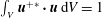
the volume of the computational domain. Finally, the structural sensitivity is defined as the region where a local perturbation of the equation system results in the largest drift of the eigenvalue, and is given by
$V$
the volume of the computational domain. Finally, the structural sensitivity is defined as the region where a local perturbation of the equation system results in the largest drift of the eigenvalue, and is given by
 $|\boldsymbol{u}||\boldsymbol{u}^{+}|$
. Here, the structural sensitivity is interpreted as the core of the instability or wavemaker (Giannetti & Luchini Reference Giannetti and Luchini2007).
$|\boldsymbol{u}||\boldsymbol{u}^{+}|$
. Here, the structural sensitivity is interpreted as the core of the instability or wavemaker (Giannetti & Luchini Reference Giannetti and Luchini2007).
4 Numerical methods
Two numerical codes have been used in this study. The Nek5000 code (Fischer Reference Fischer1997; Fischer, Lottes & Kerkemeier Reference Fischer, Lottes and Kerkemeier2008) was used for time integration of the nonlinear Navier–Stokes equations, which generated the DNS results and the POD modes presented in § 5.1. The global mode results without eddy viscosity included in appendix A were also obtained using Nek5000. The global mode results in the bulk of the manuscript were obtained by using the finite element package FreeFem++ (Hecht Reference Hecht2012). The variational formulation of the direct global mode equations including variable viscosity was derived and implemented in this work.
4.1 Nonlinear simulations and POD
Nek5000 is based on a spectral element method (Maday & Patera Reference Maday, Patera and Noor1989), which combines the accuracy of spectral methods with the flexibility of finite element methods. For details about the code implementation see Maday & Patera (Reference Maday, Patera and Noor1989). The same implementation including the Arnoldi method for modes in appendix A was used also in Lashgari et al. (Reference Lashgari, Tammisola, Citro, Brandt and Juniper2014).
In the DNS, the nonlinear Navier–Stokes equations were integrated forward in time for 481 non-dimensional time units, corresponding to around 40 flow through times from the nozzle inlet to the chamber exit. This simulation was run on high-performance computing clusters using between 256 and 1024 cores in parallel, and required over 100 000 CPU hours to complete. The time integration was performed by an explicit second-order extrapolation for the nonlinear terms, and an implicit second-order backwards-differentiation for the viscous terms, as in previous turbulent diffuser studies in Nek5000 (Ohlsson et al.
Reference Ohlsson, Schlatter, Fischer and Henningson2010). The non-dimensional time step was kept at
 ${\rm\Delta}t=1\times 10^{-4}$
to satisfy the Courant–Friedrichs–Lewy (CFL) condition. Our accuracy in time integration should compare well with other turbulent flow studies with spectral element methods, for example Ohlsson et al. (Reference Ohlsson, Schlatter, Fischer and Henningson2010).
${\rm\Delta}t=1\times 10^{-4}$
to satisfy the Courant–Friedrichs–Lewy (CFL) condition. Our accuracy in time integration should compare well with other turbulent flow studies with spectral element methods, for example Ohlsson et al. (Reference Ohlsson, Schlatter, Fischer and Henningson2010).
The computational grid used for the DNS had 58 720 spectral elements of order
 $p=6$
, giving 12.7 million grid points. The grid nearest the centreline contains a cylindrical region with a stretched Cartesian grid, similar to the grid used for a DNS of pipe flow in Nek5000 (El-Khoury et al.
Reference El-Khoury, Schlatter, Noorani, Fischer, Breethouwer and Johansson2013). In the present grid, this region contains 128 elements over the axial cross-section, and extends from
$p=6$
, giving 12.7 million grid points. The grid nearest the centreline contains a cylindrical region with a stretched Cartesian grid, similar to the grid used for a DNS of pipe flow in Nek5000 (El-Khoury et al.
Reference El-Khoury, Schlatter, Noorani, Fischer, Breethouwer and Johansson2013). In the present grid, this region contains 128 elements over the axial cross-section, and extends from
 $r=0$
to the outer radius of the inner pipe at
$r=0$
to the outer radius of the inner pipe at
 $r=0.14$
, where it attaches to an outer cylindrical grid. For
$r=0.14$
, where it attaches to an outer cylindrical grid. For
 $r>0.14$
, the grid is fully cylindrical with 32 elements over the circumference, which leads to a denser element distribution closer to the centreline where most of the interesting dynamics occur, and a coarser element distribution near the outer wall of the combustion chamber.
$r>0.14$
, the grid is fully cylindrical with 32 elements over the circumference, which leads to a denser element distribution closer to the centreline where most of the interesting dynamics occur, and a coarser element distribution near the outer wall of the combustion chamber.

Figure 2. Vorticity (helicity) from DNS at different axial cross-sections. The mesh is shown in red on top. This shows that the vorticity is continuous across the element boundaries, which is a sign of adequate resolution in spectral element method simulations of turbulent flows. (a) Typical contour upstream in the chamber (
 $z=0.2$
). (b) Typical contour downstream in the chamber (
$z=0.2$
). (b) Typical contour downstream in the chamber (
 $z=4$
). (c) Contours at
$z=4$
). (c) Contours at
 $z=4$
in a different colourscale (see colourbar), emphasizing regions of weak helicity.
$z=4$
in a different colourscale (see colourbar), emphasizing regions of weak helicity.
This study focuses on the large-scale structures, especially the precessing vortex core, so detailed turbulence statistics such as wavenumber spectra (which would require storing a huge number of snapshots) have not been computed. To ensure that the resolution is sufficient for the task at hand, the following checks have been made on the nonlinear simulation results. First, we investigated the sensitivity of the precessing vortex core to the mesh resolution by decreasing the polynomial order inside each element. Going from
 $p=6$
to
$p=6$
to
 $p=5$
(42 % less degrees of freedom), the frequency from PSD signals of the precessing vortex core remained unaltered at
$p=5$
(42 % less degrees of freedom), the frequency from PSD signals of the precessing vortex core remained unaltered at
 $St=0.67$
. Only when going from
$St=0.67$
. Only when going from
 $p=6$
to
$p=6$
to
 $p=4$
(70 % less degrees of freedom), did the frequency change slightly to
$p=4$
(70 % less degrees of freedom), did the frequency change slightly to
 $St=0.70$
. The frequency obtained with
$St=0.70$
. The frequency obtained with
 $p=6$
is also exactly the same as in experiments of Midgley et al. (Reference Midgley, Spencer and McGuirk2005) at much higher Reynolds number, confirming that the same physics is present. Furthermore, instantaneous velocity contours (showing the precessing vortex core) were confirmed to remain qualitatively the same with the coarser mesh. Finally, we investigated to what extent the turbulent motions are captured. In spectral element methods, the derivatives are not continuous across the spectral element boundaries, but become very close to continuous with increasing resolution. Therefore, in DNS using spectral element methods, a good indicator of adequate resolution of the turbulence is whether or not the vorticity or helicity fields look continuous across element boundaries (e.g. El-Khoury et al.
Reference El-Khoury, Schlatter, Noorani, Fischer, Breethouwer and Johansson2013). Figure 2 shows typical contours of the helicity in the same mesh used in the DNS in this paper. No discontinuities are seen across the element boundaries. Furthermore, the vorticity shows the expected physical trends. Upstream in the chamber (figure 2
a), we observe fine-scale vorticity, particularly in the vortex core, surrounded by a thin ring of vorticity originating at the inlet wall (
$p=6$
is also exactly the same as in experiments of Midgley et al. (Reference Midgley, Spencer and McGuirk2005) at much higher Reynolds number, confirming that the same physics is present. Furthermore, instantaneous velocity contours (showing the precessing vortex core) were confirmed to remain qualitatively the same with the coarser mesh. Finally, we investigated to what extent the turbulent motions are captured. In spectral element methods, the derivatives are not continuous across the spectral element boundaries, but become very close to continuous with increasing resolution. Therefore, in DNS using spectral element methods, a good indicator of adequate resolution of the turbulence is whether or not the vorticity or helicity fields look continuous across element boundaries (e.g. El-Khoury et al.
Reference El-Khoury, Schlatter, Noorani, Fischer, Breethouwer and Johansson2013). Figure 2 shows typical contours of the helicity in the same mesh used in the DNS in this paper. No discontinuities are seen across the element boundaries. Furthermore, the vorticity shows the expected physical trends. Upstream in the chamber (figure 2
a), we observe fine-scale vorticity, particularly in the vortex core, surrounded by a thin ring of vorticity originating at the inlet wall (
 $r=0.5$
). Near the downstream wall of the chamber (figure 2
b), the vorticity has larger scales and is smoothly distributed along the whole radial extent, although it is still strongest near the centre.
$r=0.5$
). Near the downstream wall of the chamber (figure 2
b), the vorticity has larger scales and is smoothly distributed along the whole radial extent, although it is still strongest near the centre.
The mean flows in the present study were computed by continuously time-averaging the velocity fields at every 10th time step over a time period of
 $150$
non-dimensional units. The mean flow was also averaged over the azimuthal direction, by interpolating the values at every grid point
$150$
non-dimensional units. The mean flow was also averaged over the azimuthal direction, by interpolating the values at every grid point
 $(z_{n},r_{n},{\it\theta}_{n})$
into
$(z_{n},r_{n},{\it\theta}_{n})$
into
 $(z_{n},r_{n},k2{\rm\pi}/32)$
,
$(z_{n},r_{n},k2{\rm\pi}/32)$
,
 $k=1,\ldots ,32$
, and taking the average over all
$k=1,\ldots ,32$
, and taking the average over all
 $k$
.
$k$
.
The POD modes were computed based on two different series of snapshots from DNS as follows. First, a series of 153 snapshots over a long time interval,
 $T=153$
, was saved and used to obtain the spatial shapes. A long time interval between the snapshots,
$T=153$
, was saved and used to obtain the spatial shapes. A long time interval between the snapshots,
 ${\rm\Delta}t=0.5$
, was chosen to make them statistically independent. Second, a shorter series of frequently spaced snapshots,
${\rm\Delta}t=0.5$
, was chosen to make them statistically independent. Second, a shorter series of frequently spaced snapshots,
 ${\rm\Delta}t=0.03$
apart, was used to obtain the mode frequencies. In both cases the procedure was as follows. First, the mean velocity field
${\rm\Delta}t=0.03$
apart, was used to obtain the mode frequencies. In both cases the procedure was as follows. First, the mean velocity field
 $\overline{\boldsymbol{U}}$
(obtained earlier) was subtracted from every snapshot. Subtracting the mean flow before performing the POD removes the mean flow mode, which otherwise would be the highest-energy mode. A similar zero-frequency mode will however be obtained at a lower energy, representing the difference between the mean flow averaged over all time steps, and the average over a finite number of snapshots. The snapshots with mean flow subtracted were then saved only on the part of the grid extending from
$\overline{\boldsymbol{U}}$
(obtained earlier) was subtracted from every snapshot. Subtracting the mean flow before performing the POD removes the mean flow mode, which otherwise would be the highest-energy mode. A similar zero-frequency mode will however be obtained at a lower energy, representing the difference between the mean flow averaged over all time steps, and the average over a finite number of snapshots. The snapshots with mean flow subtracted were then saved only on the part of the grid extending from
 $z=-1$
to
$z=-1$
to
 $z=4$
in the axial direction, and with a lower polynomial order
$z=4$
in the axial direction, and with a lower polynomial order
 $p=4$
. This was done in order to save memory so that postprocessing in Matlab became possible, and in order to focus on the region where the coherent structures were visible. Next, the snapshots were uploaded into Matlab and a matrix formed with these columns:
$p=4$
. This was done in order to save memory so that postprocessing in Matlab became possible, and in order to focus on the region where the coherent structures were visible. Next, the snapshots were uploaded into Matlab and a matrix formed with these columns:
 $$\begin{eqnarray}\unicode[STIX]{x1D653}\unicode[STIX]{x1D653}=[\boldsymbol{U}(t_{0})-\overline{\boldsymbol{U}},\boldsymbol{U}(t_{0}+{\it\delta}t)-\overline{\boldsymbol{U}},\ldots ,\boldsymbol{U}(t_{0}+T)-\overline{\boldsymbol{U}}].\end{eqnarray}$$
The POD modes were obtained from the singular value decomposition of the snapshot matrix:
 $\unicode[STIX]{x1D653}\unicode[STIX]{x1D653}=\boldsymbol{U}\unicode[STIX]{x1D64E}\boldsymbol{V}^{\text{T}}$
, where
$\unicode[STIX]{x1D653}\unicode[STIX]{x1D653}=\boldsymbol{U}\unicode[STIX]{x1D64E}\boldsymbol{V}^{\text{T}}$
, where
 $\boldsymbol{U}$
contains the POD modes, the energies are obtained using
$\boldsymbol{U}$
contains the POD modes, the energies are obtained using
 $\unicode[STIX]{x1D64E}$
, and the time coefficients are
$\unicode[STIX]{x1D64E}$
, and the time coefficients are
 $\boldsymbol{a}=\unicode[STIX]{x1D64E}\boldsymbol{V}^{\text{T}}$
.
$\boldsymbol{a}=\unicode[STIX]{x1D64E}\boldsymbol{V}^{\text{T}}$
.
4.2 Extraction of the eddy viscosity from POD
To compute the turbulent Reynolds stresses in DNS, we used the already computed POD modes from the long time series. First, the snapshot matrix
 $\unicode[STIX]{x1D653}\unicode[STIX]{x1D653}$
was reconstructed while setting to zero the time coefficients for the first four POD modes, which represent coherent structures, and the fifth POD mode, which represents the mean flow:
$\unicode[STIX]{x1D653}\unicode[STIX]{x1D653}$
was reconstructed while setting to zero the time coefficients for the first four POD modes, which represent coherent structures, and the fifth POD mode, which represents the mean flow:
 $$\begin{eqnarray}\unicode[STIX]{x1D653}\unicode[STIX]{x1D653}_{new}=\mathop{\sum }_{k=6}^{N}\boldsymbol{U}(\boldsymbol{ : },k)\boldsymbol{a}(k,\boldsymbol{ : }).\end{eqnarray}$$
Now, every column of
 $\unicode[STIX]{x1D653}\unicode[STIX]{x1D653}_{new}$
is a snapshot of the original time series excluding the coherent structures, which we label a ‘reduced snapshot’. Second, the Reynolds stresses were computed and an average taken over all reduced snapshots. Third, the stresses were transformed to cylindrical coordinates and averaged over the azimuthal direction in the same way as the mean flow. Finally, they were interpolated back to Cartesian coordinates, and combined with mean flow stresses to form the product shown in (3.7). It was observed that the ratio between the Reynolds stresses and mean flow stresses can become ill-conditioned in regions where both of them are extremely small. Hence, a cutoff of
$\unicode[STIX]{x1D653}\unicode[STIX]{x1D653}_{new}$
is a snapshot of the original time series excluding the coherent structures, which we label a ‘reduced snapshot’. Second, the Reynolds stresses were computed and an average taken over all reduced snapshots. Third, the stresses were transformed to cylindrical coordinates and averaged over the azimuthal direction in the same way as the mean flow. Finally, they were interpolated back to Cartesian coordinates, and combined with mean flow stresses to form the product shown in (3.7). It was observed that the ratio between the Reynolds stresses and mean flow stresses can become ill-conditioned in regions where both of them are extremely small. Hence, a cutoff of
 $10^{-4}$
was employed on both stresses, and a cutoff of 100 was employed on the turbulent viscosity.
$10^{-4}$
was employed on both stresses, and a cutoff of 100 was employed on the turbulent viscosity.
4.3 Linear global modes
We implemented the global cylindrical linear stability equations with an azimuthal wavenumber
 $m$
and a variable viscosity using the discretization and coding environment provided by FreeFem++ in combination with ARPACK, in the same way as Tammisola et al. (Reference Tammisola, Giannetti, Citro and Juniper2014) for a planar Cartesian geometry. The adjoint stability equations were also derived and implemented (continuous adjoint approach) in the case of molecular viscosity. For the variable viscosity case, the adjoint equations were not derived explicitly, but the adjoint modes were obtained using the conjugate transpose of the direct system matrix (discrete adjoint approach).
$m$
and a variable viscosity using the discretization and coding environment provided by FreeFem++ in combination with ARPACK, in the same way as Tammisola et al. (Reference Tammisola, Giannetti, Citro and Juniper2014) for a planar Cartesian geometry. The adjoint stability equations were also derived and implemented (continuous adjoint approach) in the case of molecular viscosity. For the variable viscosity case, the adjoint equations were not derived explicitly, but the adjoint modes were obtained using the conjugate transpose of the direct system matrix (discrete adjoint approach).
The spatial domain was discretized by a triangular finite elements mesh using a Delaunay–Voronoi algorithm, leading to a mesh with 213 620 triangles and 108 486 vertices. We employed the pair
 $\mathbb{P}_{2}{-}\mathbb{P}_{1}$
, consisting of piece-wise quadratic velocities and piece-wise linear pressure (Taylor–Hood elements), leading to
$\mathbb{P}_{2}{-}\mathbb{P}_{1}$
, consisting of piece-wise quadratic velocities and piece-wise linear pressure (Taylor–Hood elements), leading to
 $10^{6}$
degrees of freedom. The Nek5000 code was also used to compute modes without eddy viscosity in appendix A. The eigenmodes in Nek5000 were computed directly from the ansatz
$10^{6}$
degrees of freedom. The Nek5000 code was also used to compute modes without eddy viscosity in appendix A. The eigenmodes in Nek5000 were computed directly from the ansatz
 $\boldsymbol{u}(x,y,z,t)=\hat{\boldsymbol{u}}(x,y,z)\exp ({\it\sigma}t)$
, without setting an azimuthal wavenumber. This means that the obtained eigenspectrum from Nek5000 was a combination of all azimuthal wavenumbers. The two codes were cross-validated against each other, and the resolution independence of the eigenvalues tested, using molecular viscosity. The eigenvalues are documented in table 1 in appendix A.
$\boldsymbol{u}(x,y,z,t)=\hat{\boldsymbol{u}}(x,y,z)\exp ({\it\sigma}t)$
, without setting an azimuthal wavenumber. This means that the obtained eigenspectrum from Nek5000 was a combination of all azimuthal wavenumbers. The two codes were cross-validated against each other, and the resolution independence of the eigenvalues tested, using molecular viscosity. The eigenvalues are documented in table 1 in appendix A.

Figure 3. Mean flow from DNS at
 $Re=4800$
: (a) axial velocity, (b) radial velocity, (c) azimuthal velocity.
$Re=4800$
: (a) axial velocity, (b) radial velocity, (c) azimuthal velocity.

Figure 4. Mean flow from DNS at
 $Re=4800$
, contours of the axial–radial velocity streamfunction.
$Re=4800$
, contours of the axial–radial velocity streamfunction.

Figure 5. Instantaneous velocity from DNS at
 $Re=4800$
, axial velocity at a cross-section of the injector, at two different time instants (a and b). Light colours indicate high velocity positive in the streamwise direction, and dark colours negative velocity in the streamwise direction. Contours of (half of) the injector are also visible.
$Re=4800$
, axial velocity at a cross-section of the injector, at two different time instants (a and b). Light colours indicate high velocity positive in the streamwise direction, and dark colours negative velocity in the streamwise direction. Contours of (half of) the injector are also visible.

Figure 6. (a) Illustration showing the location of the probe signals A, B and C in the
 $z$
–
$z$
–
 $r$
plane (eight other probes were also recorded). (b) PSD spectrum of probe A at
$r$
plane (eight other probes were also recorded). (b) PSD spectrum of probe A at
 $z=0.25$
,
$z=0.25$
,
 $r=0$
, (c) PSD spectrum of probe B at
$r=0$
, (c) PSD spectrum of probe B at
 $z=0.05$
,
$z=0.05$
,
 $r=0.35$
(
$r=0.35$
(
 ${\it\theta}={\rm\pi}/4$
) (d) PSD spectrum of probe C at
${\it\theta}={\rm\pi}/4$
) (d) PSD spectrum of probe C at
 $z=1$
,
$z=1$
,
 $r=1.5$
(
$r=1.5$
(
 ${\it\theta}={\rm\pi}$
).
${\it\theta}={\rm\pi}$
).

Figure 7. POD mode 1 and mode 3 from the two leading mode pairs (mode 2 is the same as mode 1 with
 ${\rm\pi}/2$
phase difference, and mode 4 is the same as mode 3 with
${\rm\pi}/2$
phase difference, and mode 4 is the same as mode 3 with
 ${\rm\pi}/4$
phase difference): (a) mode 1, 3D contour of axial velocity; (b) the same for mode 3; (c) mode 1, axial velocity at the azimuthal cross-section at
${\rm\pi}/4$
phase difference): (a) mode 1, 3D contour of axial velocity; (b) the same for mode 3; (c) mode 1, axial velocity at the azimuthal cross-section at
 ${\it\theta}={\rm\pi}/2$
; (d) the same for mode 3; (e) mode 1, the same as (c) but filtered by FFT in the azimuthal direction; (f) the same for mode 3.
${\it\theta}={\rm\pi}/2$
; (d) the same for mode 3; (e) mode 1, the same as (c) but filtered by FFT in the azimuthal direction; (f) the same for mode 3.

Figure 8. The leading Fourier component only (
 $m=1$
) for the first POD mode pair: mode 1 (a,c,e) and mode 2 (b,d, f). (a,b) Axial, (c,d) radial and (e,f) azimuthal velocity.
$m=1$
) for the first POD mode pair: mode 1 (a,c,e) and mode 2 (b,d, f). (a,b) Axial, (c,d) radial and (e,f) azimuthal velocity.

Figure 9. The leading Fourier component only (
 $m=2$
) for the second POD mode pair: mode 3 (a,c,e) and mode 4 (b,d, f). (a,b) Axial, (c,d) radial and (e,f) azimuthal velocity.
$m=2$
) for the second POD mode pair: mode 3 (a,c,e) and mode 4 (b,d, f). (a,b) Axial, (c,d) radial and (e,f) azimuthal velocity.

Figure 10. (a) The FFT coefficients of the chronos (time-domain) part of the first 11 POD modes, multiplied by their respective energies (see legend for lines/markers). The figure illustrates that POD mode pair 1–2 (blue online) is relatively monofrequent, and also is the by far most energetic coherent structure in the flow. A weaker coherent structure is seen in POD mode pair 3–4 (red online). (b) The same but shown in a logarithmic scale on both axes.
5 Results
5.1 Nonlinear simulation
Here, we consider the nonlinear dynamics of the flow in the fuel injector at
 $Re=4800$
. We start from the mean flow, i.e. the time-averaged velocity field from DNS, shown in figure 3 (velocity components) and 4 (streamlines). The flow develops two large recirculation zones inside the combustion chamber, which is characteristic of swirl injectors (Syred Reference Syred2006). The inner wall separation develops into a central zone that starts near the centreline and expands radially, covering the whole back wall. This zone is in turn divided into two recirculation bubbles: one closer to the inlet and one closer to the back wall. Another large coaxial recirculation zone develops near the upstream wall of the combustion chamber through separation at the outer edge of the coaxial inlet and confinement by the upper wall. The reason for the formation of the central recirculation zone is analogous to the formation of an axisymmetric vortex breakdown bubble in a swirling jet, explained by Syred (Reference Syred2006) in the case of a straight combustor. For a swirling jet, the radial expansion of the potential vortex core, with its associated normal pressure gradient, creates an adverse pressure gradient along the centreline, and the flow separates, forming a vortex breakdown bubble. For the Turbomeca coaxial fuel injector, the flow separates inside the nozzle for two reasons. The first reason is that axisymmetric vortex breakdown occurs when the combination of swirl (tangential velocity) and the Reynolds number are high enough (Ruith et al.
Reference Ruith, Chen, Meiburg and Maxworthy2003). In the upstream, contracting part of the inlet, the flow contracts in the radial direction (the radial velocity is shown in figure 3
b), creating a high magnitude of swirl (3
c) near the inner wall of the outer channel due to the conservation of angular momentum, and the swirl profile there resembles a potential vortex. The axial flow velocity (3
a) is increased in the contraction by mass conservation, and hence the local Reynolds number increases. The second reason for vortex breakdown to occur inside the nozzle is that the area of the nozzle increases again with the straight outer wall at
$Re=4800$
. We start from the mean flow, i.e. the time-averaged velocity field from DNS, shown in figure 3 (velocity components) and 4 (streamlines). The flow develops two large recirculation zones inside the combustion chamber, which is characteristic of swirl injectors (Syred Reference Syred2006). The inner wall separation develops into a central zone that starts near the centreline and expands radially, covering the whole back wall. This zone is in turn divided into two recirculation bubbles: one closer to the inlet and one closer to the back wall. Another large coaxial recirculation zone develops near the upstream wall of the combustion chamber through separation at the outer edge of the coaxial inlet and confinement by the upper wall. The reason for the formation of the central recirculation zone is analogous to the formation of an axisymmetric vortex breakdown bubble in a swirling jet, explained by Syred (Reference Syred2006) in the case of a straight combustor. For a swirling jet, the radial expansion of the potential vortex core, with its associated normal pressure gradient, creates an adverse pressure gradient along the centreline, and the flow separates, forming a vortex breakdown bubble. For the Turbomeca coaxial fuel injector, the flow separates inside the nozzle for two reasons. The first reason is that axisymmetric vortex breakdown occurs when the combination of swirl (tangential velocity) and the Reynolds number are high enough (Ruith et al.
Reference Ruith, Chen, Meiburg and Maxworthy2003). In the upstream, contracting part of the inlet, the flow contracts in the radial direction (the radial velocity is shown in figure 3
b), creating a high magnitude of swirl (3
c) near the inner wall of the outer channel due to the conservation of angular momentum, and the swirl profile there resembles a potential vortex. The axial flow velocity (3
a) is increased in the contraction by mass conservation, and hence the local Reynolds number increases. The second reason for vortex breakdown to occur inside the nozzle is that the area of the nozzle increases again with the straight outer wall at
 $z>-0.5$
, strengthening the expansion of the vortex core (3
c).
$z>-0.5$
, strengthening the expansion of the vortex core (3
c).
The smooth mean flow is very different from the instantaneous flow structures that are shown in figure 5(a,b). Snapshots of the axial velocity are shown at two different time instants, over an azimuthal cross-section of the domain (
 ${\it\theta}={\rm\pi}/2$
). The flow starts as laminar through the coaxial inlet, but when it separates at its inner wall near the combustion chamber, the separation point oscillates back and forth towards the centreline in a violent spiralling motion. This large-scale motion is visible in (b), where the axial velocity field is clearly asymmetric with respect to the centreline. The same region in (a) displays a Kelvin–Helmholtz-like wavy pattern which is symmetric with respect to the centreline over the cross-section, indicating an oscillation with an even azimuthal wavenumber. Apart from the large scales, both subfigures show a continuous range of smaller spatial scales. The flow at the separation zone near the central inlet, and downstream in the combustion chamber, becomes turbulent.
${\it\theta}={\rm\pi}/2$
). The flow starts as laminar through the coaxial inlet, but when it separates at its inner wall near the combustion chamber, the separation point oscillates back and forth towards the centreline in a violent spiralling motion. This large-scale motion is visible in (b), where the axial velocity field is clearly asymmetric with respect to the centreline. The same region in (a) displays a Kelvin–Helmholtz-like wavy pattern which is symmetric with respect to the centreline over the cross-section, indicating an oscillation with an even azimuthal wavenumber. Apart from the large scales, both subfigures show a continuous range of smaller spatial scales. The flow at the separation zone near the central inlet, and downstream in the combustion chamber, becomes turbulent.
To give an idea of the temporal scales, the temporal probe signal data from different parts of the domain is shown next. The power spectral density (PSD) of the instantaneous azimuthal velocity is shown in figure 6. The probe at A in figure 6(a) at the centreline near the chamber inlet (
 $z=0.5$
,
$z=0.5$
,
 $r=0$
) shows a clear peak at Strouhal number
$r=0$
) shows a clear peak at Strouhal number
 $St=0.67$
from the oscillating separation point. This value is exactly the same as in experiments of Midgley et al. (Reference Midgley, Spencer and McGuirk2005) at higher
$St=0.67$
from the oscillating separation point. This value is exactly the same as in experiments of Midgley et al. (Reference Midgley, Spencer and McGuirk2005) at higher
 $Re$
. The probe at B in figure 6(b) shows two peaks: a large sharp peak
$Re$
. The probe at B in figure 6(b) shows two peaks: a large sharp peak
 $St=0.67$
and a small bump at
$St=0.67$
and a small bump at
 $St=1.45$
(
$St=1.45$
(
 $St=1.39$
in experiments of Midgley et al. (Reference Midgley, Spencer and McGuirk2005)). The probe at C in figure 6(c) shows no visible peaks but only broadband turbulence.
$St=1.39$
in experiments of Midgley et al. (Reference Midgley, Spencer and McGuirk2005)). The probe at C in figure 6(c) shows no visible peaks but only broadband turbulence.
To characterize the coherent structures behind the spectral peak and the bump, we have performed proper orthogonal decomposition (POD) on two different series of snapshots, as explained in § 4.2, the first to obtain the spatial structures and the second to resolve the temporal frequencies. The two most energetic structures from POD are contained in two mode pairs: the first mode pair (POD modes 1 and 2) accounts for 17.9 % of the total energy, and the second mode pair (modes 3 and 4) for 5.4 %. The following two POD mode pairs (6–9) have a spiralling structure (
 $m=1$
), and each contribute 2 % of the energy. The POD mode 5 is the remnant of the zero-frequency mean flow mode, as explained in § 4.1.
$m=1$
), and each contribute 2 % of the energy. The POD mode 5 is the remnant of the zero-frequency mean flow mode, as explained in § 4.1.
As is typical for POD modes of oscillating flows, the two modes in each pair represent the same oscillation but with an azimuthal phase shift between them. This indicates that each mode pair represents one azimuthally travelling wave (where the group speed may be zero or finite). Mode 1 is shown in figure 7(a,c,e), and mode 3 in (b,d,e). In (a,b), 3D contours of the axial velocity are shown, as seen from the front of the injector. This clearly shows that the first mode pair (a) depicts the precessing vortex core (
 $m=1$
), and the second mode pair (b) reveals a double-helical mode (
$m=1$
), and the second mode pair (b) reveals a double-helical mode (
 $m=2$
). Both of these structures were seen in previous experiments (Midgley et al.
Reference Midgley, Spencer and McGuirk2005) and LES (Dunham et al.
Reference Dunham, Spencer, McGuirk and Dianat2008), where both modes had equal magnitudes in the PSD spectrum of the inlet probe signal. At
$m=2$
). Both of these structures were seen in previous experiments (Midgley et al.
Reference Midgley, Spencer and McGuirk2005) and LES (Dunham et al.
Reference Dunham, Spencer, McGuirk and Dianat2008), where both modes had equal magnitudes in the PSD spectrum of the inlet probe signal. At
 $Re=4800$
, however, the precessing vortex core dominates over the double-helical mode in both the PSD spectrum of the probe signals, and in the POD energies.
$Re=4800$
, however, the precessing vortex core dominates over the double-helical mode in both the PSD spectrum of the probe signals, and in the POD energies.
Despite the structures still being noisy due to the limited number of snapshots, the azimuthal cross-sections shown in figure 7(c,d) give a picture of the mode shapes. First, both modes are efficiently contained in the region
 $z=-1$
to
$z=-1$
to
 $z=3$
, diffusing into the turbulence downstream. Second, the wavelength of the precessing vortex core (c) seems to be longer (
$z=3$
, diffusing into the turbulence downstream. Second, the wavelength of the precessing vortex core (c) seems to be longer (
 ${\it\lambda}\approx 2$
near the chamber inlet) than the double-helical mode (d,
${\it\lambda}\approx 2$
near the chamber inlet) than the double-helical mode (d,
 ${\it\lambda}\approx 1.5$
). The wavelengths were extracted from these figures manually as the distance between two consecutive negative peaks (dark colour) in the wave propagation direction.
${\it\lambda}\approx 1.5$
). The wavelengths were extracted from these figures manually as the distance between two consecutive negative peaks (dark colour) in the wave propagation direction.
To improve the spatial resolution of the POD modes, for comparisons with global modes later on, we have used the knowledge of their azimuthal wavenumber and filtered them by a Fourier decomposition in the azimuthal direction, where only the
 $m=1$
component was kept for modes 1–2, and the
$m=1$
component was kept for modes 1–2, and the
 $m=2$
component for modes 3–4. This approach increases the amount of available data, as many azimuthal cross-sections are used to determine each mode shape, rather than only one cross-section. In addition, it acts as an azimuthal low-pass filter. The effect of this procedure is similar to taking the azimuthal average of DNS mean flows to improve their quality. The mode shape after the azimuthal filtering becomes substantially smoother and more well defined, while retaining all the large-scale features, as can be seen in figure 7(e, f). All velocity components of the azimuthally filtered POD modes are shown for reference in figures 8 (modes 1 and 2), and 9 (modes 3 and 4). From these figures, the detailed structure of the two POD mode pairs can be seen.
$m=2$
component for modes 3–4. This approach increases the amount of available data, as many azimuthal cross-sections are used to determine each mode shape, rather than only one cross-section. In addition, it acts as an azimuthal low-pass filter. The effect of this procedure is similar to taking the azimuthal average of DNS mean flows to improve their quality. The mode shape after the azimuthal filtering becomes substantially smoother and more well defined, while retaining all the large-scale features, as can be seen in figure 7(e, f). All velocity components of the azimuthally filtered POD modes are shown for reference in figures 8 (modes 1 and 2), and 9 (modes 3 and 4). From these figures, the detailed structure of the two POD mode pairs can be seen.
The above long-time snapshot series has a long time interval between consecutive snapshots (
 ${\rm\Delta}T=1$
), which prevents us from extracting frequency information from it. To obtain the frequency content of the most energetic structures, a second POD was performed with 864 frequently spaced snapshots, and a fast Fourier transform (FFT) taken on their time coefficients. The spatial shapes of modes 1–4 were nearly identical to the long time series. The peak amplitudes of the modes gave the frequency
${\rm\Delta}T=1$
), which prevents us from extracting frequency information from it. To obtain the frequency content of the most energetic structures, a second POD was performed with 864 frequently spaced snapshots, and a fast Fourier transform (FFT) taken on their time coefficients. The spatial shapes of modes 1–4 were nearly identical to the long time series. The peak amplitudes of the modes gave the frequency
 $0.70\pm 0.06$
for the precessing vortex core mode (POD mode 1–2), and
$0.70\pm 0.06$
for the precessing vortex core mode (POD mode 1–2), and
 $1.37\pm 0.06$
for the double-helical mode (POD mode 3–4).
$1.37\pm 0.06$
for the double-helical mode (POD mode 3–4).
By normalizing the FFT coefficients of POD mode
 $n$
with the energy of POD mode
$n$
with the energy of POD mode
 $n$
, it is also possible to compare the relative amplitudes from different POD modes at each frequency. The FFT coefficients for the first 11 POD modes normalized by their energies are shown in figure 10. The mode pair 1–2 has a clear high peak at
$n$
, it is also possible to compare the relative amplitudes from different POD modes at each frequency. The FFT coefficients for the first 11 POD modes normalized by their energies are shown in figure 10. The mode pair 1–2 has a clear high peak at
 $St=0.70$
, showing that this POD mode represents an efficiently monofrequent coherent structure. The mode pair 3–4 contains a broader distribution of frequencies, indicating that this mode may be a convectively unstable mode. The peak amplitude of mode 3–4 is an order of magnitude lower than that of mode 1–2. Any other modes have still an order of magnitude lower peak amplitudes (figure 10
b shows them in a double-logarithmic scale), and still broader FFT distributions. Based on this data, we draw the following two conclusions. First, the precessing vortex core (mode 1–2) is a monofrequent POD mode, and can be compared with temporal linear global modes later on. Second, the precessing vortex core is unlikely to have significant nonlinear interactions with any other coherent structure (including harmonics). However, the precessing vortex core is very likely to interact with the broadband random turbulent fluctuations, which when all added together will contain a significant amount of energy. To take the extra dissipation caused by these random fluctuations into account, we next create an eddy-viscosity model based on the bulk of (incoherent) POD modes.
$St=0.70$
, showing that this POD mode represents an efficiently monofrequent coherent structure. The mode pair 3–4 contains a broader distribution of frequencies, indicating that this mode may be a convectively unstable mode. The peak amplitude of mode 3–4 is an order of magnitude lower than that of mode 1–2. Any other modes have still an order of magnitude lower peak amplitudes (figure 10
b shows them in a double-logarithmic scale), and still broader FFT distributions. Based on this data, we draw the following two conclusions. First, the precessing vortex core (mode 1–2) is a monofrequent POD mode, and can be compared with temporal linear global modes later on. Second, the precessing vortex core is unlikely to have significant nonlinear interactions with any other coherent structure (including harmonics). However, the precessing vortex core is very likely to interact with the broadband random turbulent fluctuations, which when all added together will contain a significant amount of energy. To take the extra dissipation caused by these random fluctuations into account, we next create an eddy-viscosity model based on the bulk of (incoherent) POD modes.
6 Turbulent viscosity from DNS
To approximate the effect of turbulent dissipation and its modelling on the linear global modes in the next section, we have extracted an approximate eddy-viscosity distribution from our DNS data using the simple Newtonian eddy model, as very recently used by Oberleithner et al. (Reference Oberleithner, Stöhr, Im, Arndt and Steinberg2015), and also suggested by Mettot et al. (Reference Mettot, Sipp and Bézard2014b ). The idea is based on a triple decomposition of the turbulent flow field:
 $$\begin{eqnarray}\boldsymbol{u}_{tot}=\boldsymbol{U}+\widetilde{\boldsymbol{u}}+\boldsymbol{u}^{\prime },\end{eqnarray}$$
where
 $\boldsymbol{U}$
is the mean flow,
$\boldsymbol{U}$
is the mean flow,
 $\widetilde{\boldsymbol{u}}$
are the large-scale coherent structures, and
$\widetilde{\boldsymbol{u}}$
are the large-scale coherent structures, and
 $\boldsymbol{u}^{\prime }$
the small-scale turbulent fluctuations, which we assume can be modelled by an eddy viscosity (§ 3.1). To extract the latter from the DNS data, we first estimated that the large-scale coherent structures
$\boldsymbol{u}^{\prime }$
the small-scale turbulent fluctuations, which we assume can be modelled by an eddy viscosity (§ 3.1). To extract the latter from the DNS data, we first estimated that the large-scale coherent structures
 $\widetilde{\boldsymbol{u}}$
would be represented by the first four POD modes (the
$\widetilde{\boldsymbol{u}}$
would be represented by the first four POD modes (the
 $m=1$
and
$m=1$
and
 $m=2$
modes analysed in § 5.1). We then reconstructed the flow field using all the other POD modes while setting the time coefficients for the first four to zero, to obtain
$m=2$
modes analysed in § 5.1). We then reconstructed the flow field using all the other POD modes while setting the time coefficients for the first four to zero, to obtain
 $\boldsymbol{u}^{\prime }$
. Further, we extracted an isotropic turbulent viscosity as detailed in § 4.2. Contours of the turbulent viscosity (normalized by the molecular viscosity) are shown in figure 11. The turbulent viscosity is seen to be negligible in the upstream part of the nozzle and near the walls, while it is very high (
$\boldsymbol{u}^{\prime }$
. Further, we extracted an isotropic turbulent viscosity as detailed in § 4.2. Contours of the turbulent viscosity (normalized by the molecular viscosity) are shown in figure 11. The turbulent viscosity is seen to be negligible in the upstream part of the nozzle and near the walls, while it is very high (
 ${\it\mu}_{t}/{\it\mu}>10$
) in most parts of the combustion chamber, where turbulence kinetic energy is high and mean flow stresses comparably low due to the expansion.
${\it\mu}_{t}/{\it\mu}>10$
) in most parts of the combustion chamber, where turbulence kinetic energy is high and mean flow stresses comparably low due to the expansion.
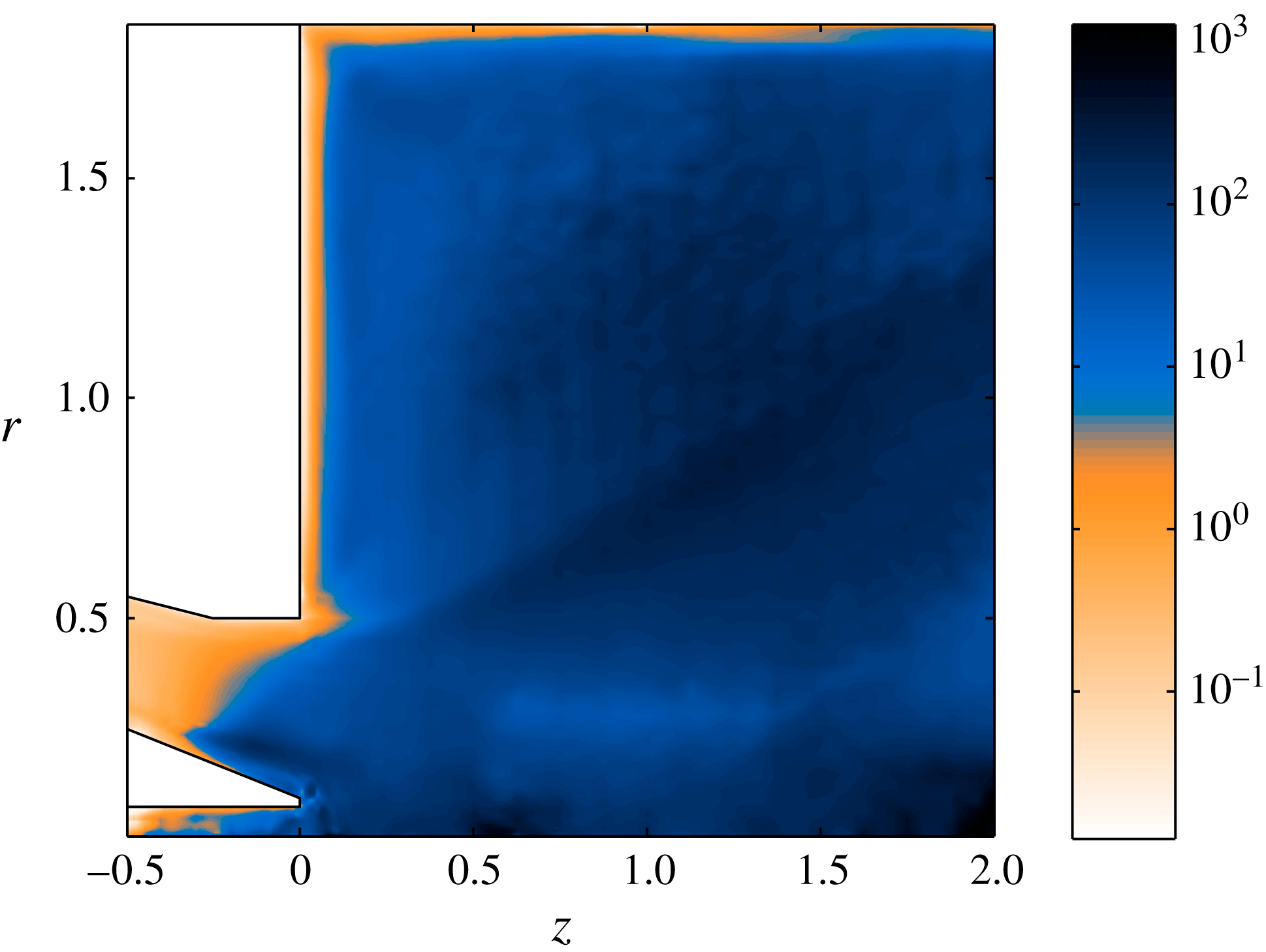
Figure 11. Contours of
 ${\it\mu}_{t}/{\it\mu}$
, where
${\it\mu}_{t}/{\it\mu}$
, where
 ${\it\mu}_{t}$
is the turbulent viscosity extracted from the POD modes excluding the coherent structures (1–4).
${\it\mu}_{t}$
is the turbulent viscosity extracted from the POD modes excluding the coherent structures (1–4).
 ${\it\mu}_{t}$
is used to form the effective Reynolds number ((3.9) and (3.7)). Observe that the contours are logarithmically spaced.
${\it\mu}_{t}$
is used to form the effective Reynolds number ((3.9) and (3.7)). Observe that the contours are logarithmically spaced.

Figure 12. The global linear eigenvalue spectrum around the DNS mean flow (figure 3) at
 $Re=4800$
: (a) modes with
$Re=4800$
: (a) modes with
 $m=1$
, (b) modes with
$m=1$
, (b) modes with
 $m=2$
.
$m=2$
.

Figure 13.
 $m=1$
mode. (a,c,e) Global mode: (a) axial, (c) radial, (e) azimuthal velocity. (b,d, f) POD mode 1 from DNS: (b) axial, (d) radial and (f) azimuthal velocity.
$m=1$
mode. (a,c,e) Global mode: (a) axial, (c) radial, (e) azimuthal velocity. (b,d, f) POD mode 1 from DNS: (b) axial, (d) radial and (f) azimuthal velocity.

Figure 14. (a) Magnitude of the adjoint velocity of the global mode representing the precessing vortex core (the direct mode shown in figure 13 a,c,e). (b) Structural sensitivity of the same precessing vortex core mode.
7 Precessing vortex core as a global mode
We now seek to identify the precessing vortex core (PVC) as a global mode, with the aim of quantifying its structural sensitivity. Structural sensitivity can indicate where in the flow the PVC originates, and where the PVC may be influenced by changes in the flow and geometry.
The linear global modes were computed in FreeFem++ around the mean flow obtained from DNS. The whole eigenvalue spectra were first computed with different azimuthal wavenumbers on the coarser mesh with
 $5.5\times 10^{5}$
degrees of freedom. The computation was then repeated using a shift around the dominant mode, on a finer mesh with
$5.5\times 10^{5}$
degrees of freedom. The computation was then repeated using a shift around the dominant mode, on a finer mesh with
 $1.23\times 10^{6}$
degrees of freedom, and the finer mesh was used to obtain results for eigenmode shapes and wavemakers. To include the effect of turbulent dissipation on the eigenmodes, the turbulent viscosity (figure 11) was used to generate a spatially varying Reynolds number
$1.23\times 10^{6}$
degrees of freedom, and the finer mesh was used to obtain results for eigenmode shapes and wavemakers. To include the effect of turbulent dissipation on the eigenmodes, the turbulent viscosity (figure 11) was used to generate a spatially varying Reynolds number
 $Re_{eff}(z,r,{\it\theta})$
. The effective Reynolds number was subsequently used in the stability computations. This is the approach in which the Reynolds stresses themselves are not linearized, named the ‘frozen eddy viscosity’ approach in § 1.
$Re_{eff}(z,r,{\it\theta})$
. The effective Reynolds number was subsequently used in the stability computations. This is the approach in which the Reynolds stresses themselves are not linearized, named the ‘frozen eddy viscosity’ approach in § 1.
The global eigenvalue spectra computed this way are shown in figure 12 for azimuthal wavenumbers
 $m=1$
(a) and
$m=1$
(a) and
 $m=2$
(b). To find oscillators, we turn our attention to the discrete global modes, separated from the continuous branch (which represents convective instabilities). Precisely one oscillator candidate is found: a
$m=2$
(b). To find oscillators, we turn our attention to the discrete global modes, separated from the continuous branch (which represents convective instabilities). Precisely one oscillator candidate is found: a
 $m=1$
mode with close to neutral growth rate. All other modes have very low growth rates. Modes at higher wavenumbers (
$m=1$
mode with close to neutral growth rate. All other modes have very low growth rates. Modes at higher wavenumbers (
 $m=3$
,
$m=3$
,
 $m=4$
) have also been computed, and have an even lower growth rate.
$m=4$
) have also been computed, and have an even lower growth rate.
To confirm that the selected global mode captures the correct physics, we compare the nearly neutral
 $m=1$
global mode with the most energetic POD mode pair, which was seen to be very close to monofrequent (figure 10). The frequency of the linear global mode is
$m=1$
global mode with the most energetic POD mode pair, which was seen to be very close to monofrequent (figure 10). The frequency of the linear global mode is
 $St=0.74$
, which compares very well with the POD mode frequency:
$St=0.74$
, which compares very well with the POD mode frequency:
 $St=0.7$
. The resulting direct global instability eigenmode with
$St=0.7$
. The resulting direct global instability eigenmode with
 $m=1$
is shown in figure 13. The global mode is shown in (a,c,e), and the corresponding POD mode from DNS in (b,d,f) for comparison. The agreement with the POD mode shapes is excellent: the wavelength matches throughout the whole domain, and the shape and amplitude distribution also agree well.
$m=1$
is shown in figure 13. The global mode is shown in (a,c,e), and the corresponding POD mode from DNS in (b,d,f) for comparison. The agreement with the POD mode shapes is excellent: the wavelength matches throughout the whole domain, and the shape and amplitude distribution also agree well.
With the goal of finding the wavemaker of the precessing vortex core more, its corresponding adjoint eigenmode has also been computed. The adjoint mode represents the optimal initial condition to excite the global mode (Chomaz Reference Chomaz2005). The magnitude of the adjoint velocity eigenmode is shown in figure 14(a). The adjoint mode is strongest inside the nozzle, along the whole extent of a shear/vorticity layer which starts at the inlet and includes the vortex breakdown location. This shows that any velocity perturbation that is on the streamline that impinges on the wavemaker region (discussed next) will have the strongest influence.
For oscillators such as the precessing vortex core, an optimal initial condition is not enough to alter the system dynamics. The eigenvalue needs to change, so the receptivity (adjoint mode) needs to overlap with a high amplitude of the direct mode. We will now overlap the direct and adjoint modes to obtain the structural sensitivity, given by the 2-norm of the structural sensitivity tensor. The structural sensitivity of the precessing vortex core is shown in figure 14(b). Knowing that the adjoint mode is strong upstream of the separation point, and the direct mode is strong downstream of the separation point, it is not surprising a posteriori that the wavemaker (structural sensitivity) resides near the separation point, which is the upstream point of the inner vortex breakdown bubble. Without prior knowledge, however, one might not have guessed that the structural sensitivity is so localized. The complicated mean flow with multiple recirculation zones (figure 4) might be expected to give rise to a range of different instability mechanisms. The sensitivity, however, points out a very specific region as the origin of the dominant instability: the vorticity layer and high-swirl region prior to the separation region near the nozzle exit.

Figure 15. Profiles in the axial location of the maximum structural sensitivity inside the nozzle (
 $z=-0.24$
): (a) mean flow velocity profile, axial (
$z=-0.24$
): (a) mean flow velocity profile, axial (
 $U_{z}$
) and swirl (
$U_{z}$
) and swirl (
 $U_{{\it\theta}}$
) components. Structural sensitivity magnitude is shown by the greyscale on top. (b) Profile of the structural sensitivity magnitude in the same axial location.
$U_{{\it\theta}}$
) components. Structural sensitivity magnitude is shown by the greyscale on top. (b) Profile of the structural sensitivity magnitude in the same axial location.
8 Instability mechanism
We will now use the structural sensitivity to investigate which instability mechanisms are active in the precessing vortex core instability.
The axial location of the maximum structural sensitivity is inside the nozzle, at
 $z=-0.24$
. Mean flow velocity profiles in the axial location of the maximum sensitivity are shown in figure 15(a). Spiral vortex breakdown is an oscillatory motion which may occur in swirling flows that have a potential core and decaying swirl in the outer region (Leibovich Reference Leibovich1978), as in the mean swirl profile shown here. Spiral vortex breakdown occurs at swirl values slightly higher than that of the steady axisymmetric breakdown. Axisymmetric breakdown is the cause of flow separation inside a nozzle in swirl injectors (Leibovich Reference Leibovich1978; Syred Reference Syred2006). This flow (figure 3) separates in the nozzle and spiral vortex breakdown is possible.
$z=-0.24$
. Mean flow velocity profiles in the axial location of the maximum sensitivity are shown in figure 15(a). Spiral vortex breakdown is an oscillatory motion which may occur in swirling flows that have a potential core and decaying swirl in the outer region (Leibovich Reference Leibovich1978), as in the mean swirl profile shown here. Spiral vortex breakdown occurs at swirl values slightly higher than that of the steady axisymmetric breakdown. Axisymmetric breakdown is the cause of flow separation inside a nozzle in swirl injectors (Leibovich Reference Leibovich1978; Syred Reference Syred2006). This flow (figure 3) separates in the nozzle and spiral vortex breakdown is possible.
The swirl number for spiral vortex breakdown is similar in different swirling flows:
 $S=0.915$
for a vortex breakdown bubble (Ruith et al.
Reference Ruith, Chen, Meiburg and Maxworthy2003; Meliga et al.
Reference Meliga, Gallaire and Chomaz2012a
) and
$S=0.915$
for a vortex breakdown bubble (Ruith et al.
Reference Ruith, Chen, Meiburg and Maxworthy2003; Meliga et al.
Reference Meliga, Gallaire and Chomaz2012a
) and
 $S=0.88$
for a swirling jet (Oberleithner et al.
Reference Oberleithner, Sieber and Nayeri2011). In the position of the wavemaker in this flow, the swirl number based on the average velocities is
$S=0.88$
for a swirling jet (Oberleithner et al.
Reference Oberleithner, Sieber and Nayeri2011). In the position of the wavemaker in this flow, the swirl number based on the average velocities is
 $Sw=1.13$
. We suggest that the precessing vortex core is a spiral vortex breakdown instability, which takes place inside the nozzle in this injector flow mainly for two reasons: (i) the contraction leads to an increase of swirl through conservation of angular momentum until the swirl number reaches a critical value, and (ii) the favourable pressure gradient (which otherwise may suppress vortex breakdown, Leibovich Reference Leibovich1978) is less strong near the nozzle outlet where the flow starts to expand radially.
$Sw=1.13$
. We suggest that the precessing vortex core is a spiral vortex breakdown instability, which takes place inside the nozzle in this injector flow mainly for two reasons: (i) the contraction leads to an increase of swirl through conservation of angular momentum until the swirl number reaches a critical value, and (ii) the favourable pressure gradient (which otherwise may suppress vortex breakdown, Leibovich Reference Leibovich1978) is less strong near the nozzle outlet where the flow starts to expand radially.
The structural sensitivity of the spiral vortex breakdown around an axisymmetric vortex breakdown bubble was studied by Qadri et al. (Reference Qadri, Mistry and Juniper2013). The structural sensitivity magnitude was high at the upstream end of the recirculation zone, with maximum amplitude at the centreline just upstream of the recirculation bubble. By considering different components of the structural sensitivity tensor, the instability mechanism was proposed to be due to the conservation of angular momentum upstream of the bubble, amplified by Kelvin–Helmholtz instability waves in the shear layer around the bubble.
In our flow, the structural sensitivity is also high just upstream of the separation point. However, the peak of the structural sensitivity in the vertical direction (light colours in figure 15) is in the shear layer. More tellingly, the peak of the structural sensitivity coincides with the inflection point in the shear layer. The whole profile of structural sensitivity magnitude as a function of vertical coordinate is shown in figure 15(b). The structural sensitivity of a parallel wake, shown in Qadri et al. (Reference Qadri, Mistry and Juniper2013), has a very similar appearance. This suggests that Kelvin–Helmholtz mechanism may be more influential for the injector flow than it is for the axisymmetric vortex breakdown bubble.

Figure 16. Magnitude of components of the structural sensitivity tensor: (a)
 $u_{z}u_{z}^{+}$
, (b)
$u_{z}u_{z}^{+}$
, (b)
 $u_{z}u_{r}^{+}$
, (c)
$u_{z}u_{r}^{+}$
, (c)
 $u_{z}u_{{\it\theta}}^{+}$
, (d)
$u_{z}u_{{\it\theta}}^{+}$
, (d)
 $u_{r}u_{z}^{+}$
, (e)
$u_{r}u_{z}^{+}$
, (e)
 $u_{r}u_{r}^{+}$
, (f)
$u_{r}u_{r}^{+}$
, (f)
 $u_{r}u_{{\it\theta}}^{+}$
, (g)
$u_{r}u_{{\it\theta}}^{+}$
, (g)
 $u_{{\it\theta}}u_{z}^{+}$
, (h)
$u_{{\it\theta}}u_{z}^{+}$
, (h)
 $u_{{\it\theta}}u_{r}^{+}$
, (i)
$u_{{\it\theta}}u_{r}^{+}$
, (i)
 $u_{{\it\theta}}u_{{\it\theta}}^{+}$
. The colourscale goes from
$u_{{\it\theta}}u_{{\it\theta}}^{+}$
. The colourscale goes from
 $0$
(dark) to
$0$
(dark) to
 $17.2$
(light).
$17.2$
(light).
In Qadri et al. (Reference Qadri, Mistry and Juniper2013), the relative importance of angular momentum conservation and Kelvin–Helmholtz instability was investigated based on the relative magnitudes of individual components of the structural sensitivity tensor
 $\unicode[STIX]{x1D61A}_{ij}=u_{i}u_{j}^{+}$
, where the index represents the axial, radial or azimuthal velocity component of the eigenmode
$\unicode[STIX]{x1D61A}_{ij}=u_{i}u_{j}^{+}$
, where the index represents the axial, radial or azimuthal velocity component of the eigenmode
 $u$
or its adjoint
$u$
or its adjoint
 $u^{+}$
. For example, the component
$u^{+}$
. For example, the component
 $\unicode[STIX]{x1D61A}_{zr}$
represents a physical feedback mechanism where the radial momentum equation is perturbed by a force proportional to
$\unicode[STIX]{x1D61A}_{zr}$
represents a physical feedback mechanism where the radial momentum equation is perturbed by a force proportional to
 $u_{z}$
(for example, axial drag). The magnitude
$u_{z}$
(for example, axial drag). The magnitude
 $\Vert \unicode[STIX]{x1D61A}_{zr}\Vert$
represents the maximal eigenvalue change caused by such a mechanism. The magnitudes of the nine components of
$\Vert \unicode[STIX]{x1D61A}_{zr}\Vert$
represents the maximal eigenvalue change caused by such a mechanism. The magnitudes of the nine components of
 $\unicode[STIX]{x1D61A}_{ij}$
are shown in figure 16(a–i). The
$\unicode[STIX]{x1D61A}_{ij}$
are shown in figure 16(a–i). The
 $\unicode[STIX]{x1D61A}_{zz}$
component dominates, as was shown to be the case for the Kelvin–Helmholtz instability of a parallel wake in Qadri et al. (Reference Qadri, Mistry and Juniper2013). In contrast to the axisymmetric vortex breakdown, the feedback from angular momentum is weaker in comparison (components
$\unicode[STIX]{x1D61A}_{zz}$
component dominates, as was shown to be the case for the Kelvin–Helmholtz instability of a parallel wake in Qadri et al. (Reference Qadri, Mistry and Juniper2013). In contrast to the axisymmetric vortex breakdown, the feedback from angular momentum is weaker in comparison (components
 $\unicode[STIX]{x1D61A}_{r{\it\theta}}$
,
$\unicode[STIX]{x1D61A}_{r{\it\theta}}$
,
 $\unicode[STIX]{x1D61A}_{rr}$
,
$\unicode[STIX]{x1D61A}_{rr}$
,
 $\unicode[STIX]{x1D61A}_{{\it\theta}r}$
,
$\unicode[STIX]{x1D61A}_{{\it\theta}r}$
,
 $\unicode[STIX]{x1D61A}_{{\it\theta}{\it\theta}}$
). This further confirms that the frequency of the global mode is selected at the shear layer inflection point by a pure Kelvin–Helmholtz mechanism. The shear layer inflection point in turn is caused by the axisymmetric vortex breakdown, and appears upstream of the breakdown (separation). This also appears to be the frequency selection of the final oscillation in the system where nonlinearities and turbulence are fully developed.
$\unicode[STIX]{x1D61A}_{{\it\theta}{\it\theta}}$
). This further confirms that the frequency of the global mode is selected at the shear layer inflection point by a pure Kelvin–Helmholtz mechanism. The shear layer inflection point in turn is caused by the axisymmetric vortex breakdown, and appears upstream of the breakdown (separation). This also appears to be the frequency selection of the final oscillation in the system where nonlinearities and turbulence are fully developed.

Figure 17. Global mode derived by including eddy viscosity (a,c) compared to the same global mode derived without eddy viscosity (b,d): (a)
 $m=1$
axial velocity, with eddy viscosity, (b)
$m=1$
axial velocity, with eddy viscosity, (b)
 $m=1$
, axial velocity, with molecular viscosity, (c) structural sensitivity, with eddy viscosity, (d) structural sensitivity, with molecular viscosity.
$m=1$
, axial velocity, with molecular viscosity, (c) structural sensitivity, with eddy viscosity, (d) structural sensitivity, with molecular viscosity.
9 Effects of excluding the turbulent dissipation on the eigenmodes
In figure 17, the axial velocity of the global mode with eddy viscosity (a) is shown alongside the leading global mode computed around the mean flow, but with only molecular viscosity (b). The latter is the quasi-laminar approach used in Mettot et al. (Reference Mettot, Sipp and Bézard2014b
). In the mode shape with molecular viscosity, we can see the boundary of the central recirculation zone, showing that the mode shape and inclination is sensitive to the local shear. In contrast, the mode shape with eddy viscosity (figure 17
a) contains vertically aligned smooth structures extending inside and outside of the recirculation zone, exactly like the POD mode. We also see that the wavelength of the global mode with molecular viscosity shortens downstream, and the mode has still a visible amplitude at
 $z=4$
, while the wavelength of the mode with eddy viscosity does not shorten and the mode disappears around
$z=4$
, while the wavelength of the mode with eddy viscosity does not shorten and the mode disappears around
 $z=3$
, in agreement with the POD mode.
$z=3$
, in agreement with the POD mode.
There is little doubt that eddy viscosity improves the agreement of the global mode shapes with the POD, and the same seems to apply to the frequencies. The mode with eddy viscosity has
 $St=0.74$
, compared to
$St=0.74$
, compared to
 $St=0.70\pm 0.06$
from DNS, and
$St=0.70\pm 0.06$
from DNS, and
 $St=0.87$
for the mode with molecular viscosity. Hence, eddy viscosity also notably improves the frequency agreement. The only drawback of the eddy viscosity is noted when looking at the mode growth rates: the stabilizing influence of turbulent dissipation is overestimated by making all eigenmodes stable. The
$St=0.87$
for the mode with molecular viscosity. Hence, eddy viscosity also notably improves the frequency agreement. The only drawback of the eddy viscosity is noted when looking at the mode growth rates: the stabilizing influence of turbulent dissipation is overestimated by making all eigenmodes stable. The
 $m=1$
mode is slightly stable with amplification rate
$m=1$
mode is slightly stable with amplification rate
 ${\it\sigma}_{r}=-0.17$
. This highlights the issue known from previous studies that it may be difficult to obtain neutral growth rates in a mean flow analysis, and this might be a problem in cases where the growth rate is used as an indicator to identify the dominant eigenmodes. It should be mentioned that the mean flow stresses used to determine the eddy-viscosity distribution include the effects from both the turbulent fluctuations and the coherent structures. To be fully consistent, the base flow for a stability computation with eddy viscosity should include the effect of turbulent dissipation but not dissipation by coherent structures (termed base flow approach in Mettot et al. (Reference Mettot, Sipp and Bézard2014b
)). A new base flow forced only by the turbulent Reynolds stresses could be computed, and this would lead to a somewhat smaller eddy viscosity, and possibly closer to neutral mode growth rates.
${\it\sigma}_{r}=-0.17$
. This highlights the issue known from previous studies that it may be difficult to obtain neutral growth rates in a mean flow analysis, and this might be a problem in cases where the growth rate is used as an indicator to identify the dominant eigenmodes. It should be mentioned that the mean flow stresses used to determine the eddy-viscosity distribution include the effects from both the turbulent fluctuations and the coherent structures. To be fully consistent, the base flow for a stability computation with eddy viscosity should include the effect of turbulent dissipation but not dissipation by coherent structures (termed base flow approach in Mettot et al. (Reference Mettot, Sipp and Bézard2014b
)). A new base flow forced only by the turbulent Reynolds stresses could be computed, and this would lead to a somewhat smaller eddy viscosity, and possibly closer to neutral mode growth rates.
Finally, as the eddy viscosity influences the mode shapes, and the mode shapes are used to construct the structural sensitivity, the eddy viscosity also has some influence on the structural sensitivity (wavemaker). The wavemakers with and without eddy viscosity are compared in figure 17(c,d). By comparing the wavemaker with eddy viscosity (c) and that with molecular viscosity (d), we see that the eddy viscosity has two effects: it makes the wavemaker more dispersed, and lifts it up slightly from the wall. Hence, the wavemaker with eddy viscosity has the same amplitude over a region starting just upstream of the separation point and ending just beyond the injector lip, while the wavemaker without eddy viscosity is more focused in the immediate vicinity of the separation point. Although the amplitude of the structural sensitivity is strongly influenced by the viscosity model used, the location of its maximum (the wavemaker region) does not change. It is inside the nozzle in the upstream part of the central recirculation zone.
The structural sensitivity gives the influence of a local perturbation of the system matrix on the eigenvalue, whether the perturbation comes from a physical or a numerical origin. Hence, apart from estimating the physical origin of the instability, the structural sensitivity also has a numerical interpretation. We can observe that eddy viscosity reduces the maximum amplitude of the structural sensitivity of the
 $m=1$
mode by an order of magnitude, from approximately 20.5 to approximately 2.5, showing that the eigenmode with molecular viscosity is more sensitive to perturbations. From the numerical solution point of view, this means that the modes without eddy viscosity, and the underlying mean flow, need to be highly resolved near the nozzle, and in particular in the region near the separation point. This makes sense based on what is known about high-Reynolds-number flows. However, the modes with eddy viscosity have a lower effective Reynolds number, and hence a more even and weaker structural sensitivity. Therefore, the use of eddy viscosity makes the global mode problem better conditioned numerically.
$m=1$
mode by an order of magnitude, from approximately 20.5 to approximately 2.5, showing that the eigenmode with molecular viscosity is more sensitive to perturbations. From the numerical solution point of view, this means that the modes without eddy viscosity, and the underlying mean flow, need to be highly resolved near the nozzle, and in particular in the region near the separation point. This makes sense based on what is known about high-Reynolds-number flows. However, the modes with eddy viscosity have a lower effective Reynolds number, and hence a more even and weaker structural sensitivity. Therefore, the use of eddy viscosity makes the global mode problem better conditioned numerically.
10 Discussion
10.1 Nonlinear interaction with harmonics and other oscillators
The role of nonlinear interaction with harmonics, and its implications for the mean flow stability results, have been investigated in the global instability community. For example, Sipp & Lebedev (Reference Sipp and Lebedev2007) considered criteria based on the coefficients of a weakly nonlinear expansion (the Landau coefficients). These criteria indicated the relative strength of the mean flow harmonic, and the second harmonic. If the nonlinearities acted more strongly to modify the mean flow, and less strongly to amplify the harmonic, then mean flow stability could give meaningful results. Criteria based on the presence of subharmonics were expressed by Mezic (Reference Mezic2013).
For the swirl injector flow in the present study, harmonics are observed neither in the PSD spectra nor in the FFT coefficients of the leading 11 POD modes. We therefore conclude that any harmonics of the precessing vortex core are unobservable compared to the mode itself. The mode is likely to interact more with the mean flow than with its second harmonic. We therefore conclude that the criteria of Sipp & Lebedev (Reference Sipp and Lebedev2007) are highly likely to be satisfied. Furthermore, the strength of the next highest spectral peak (the double-helical mode, POD mode 3–4) is an order of magnitude lower than that of the precessing vortex core. Hence, any nonlinear interactions with other oscillators or coherent structures (such as for the swirling flow in Meliga et al. (Reference Meliga, Gallaire and Chomaz2012a )) are also likely to be weak and can be ignored.
However, neither of the above studies considers the interactions between the eigenmode and the bulk of the incoherent fluctuations. The random incoherent fluctuations contain a significant part of the total energy for the swirl injector flow, and hence the precessing vortex core is highly likely to be influenced by them. This is the stochastic interaction we aim to model with the eddy viscosity.
10.2 Effect of turbulent dissipation – eddy viscosity versus molecular viscosity
First, we note that different eddy-viscosity models extracted from experimental data were tried in a local absolute instability analysis of a similar injector flow (Oberleithner et al. Reference Oberleithner, Stöhr, Im, Arndt and Steinberg2015). All eddy-viscosity models resulted in a nearly neutral growth rate. The differences between different models were less than the qualitative difference between eddy viscosity and molecular viscosity. However, the Newtonian eddy model, which is that used in the present study, provided the best match with the experiments. These findings support the hypothesis that the choice of the model for turbulent dissipation is less crucial than the choice of including it. A possible reason for this is discussed below.
The findings of the present study can be related to what is known about global stability analysis around turbulent mean flows, particularly in bluff-body flows. The effect of mean flow and dissipation has been discussed extensively in the context of reduced-order models, which is a closely related topic. The mean-field theory introduced by Noack et al. (Reference Noack, Afanasiev, Morzynski, Tadmor and Thiele2003) stated that a stability analysis around a mean flow will produce the limit cycle as a neutrally stable global mode, which was later confirmed by Barkley (Reference Barkley2006). Both authors investigated the saturation to a limit cycle oscillation of a cylinder wake at a supercritical but laminar Reynolds number. Subsequent studies have addressed the effect of small scales in a high-lift configuration (Luchtenburg et al. Reference Luchtenburg, Günther, Noack, King and Tadmor2009) and turbulent fluctuations in a complex bluff-body wake (Östh et al. Reference Östh, Noack, Krajnovic, Barros and Bore2014; Protas et al. Reference Protas, Noack and Östh2015). These studies concluded that unresolved incoherent fluctuations dissipate energy from larger scales, and this dissipation must be included in the reduced-order model in order not to overestimate the growth rates of the large scales, and even for the Galerkin approximation to converge to a finite value.
The reduced-order POD models are used to reconstruct the time evolution of the system. The above findings suggest that a time evolution around a turbulent mean can only be reproduced by including an effect of dissipation on the modes themselves. This is in line with the results of the present study. The global modes with extracted eddy viscosity gave a better agreement with DNS than the global modes with molecular viscosity. The eddy viscosity also brought the growth rate closer to neutral. Neutral growth rates would be expected according to the mean-field theory (Noack et al. Reference Noack, Afanasiev, Morzynski, Tadmor and Thiele2003). The mode shapes provide further evidence of the role of dissipation. The global modes with molecular viscosity are more localized in the shear layers, while the modes with eddy viscosity are more spread out in the vertical direction (in a better agreement with DNS). This can be compared to the instability in parallel flows such as channel flows and shear layers: the instability modes at higher Reynolds numbers have narrower and more localized shapes than those at lower Reynolds numbers. To support this hypothesis, we show instability modes at different instability and base flow Reynolds numbers in appendix B.
10.3 Structural sensitivity in turbulent external flows
The main aim of this study was to locate the structural sensitivity of the precessing vortex core. Structural sensitivity has been computed in a few earlier studies in external, non-swirling turbulent flows. Very recently, it was shown (Mettot et al.
Reference Mettot, Sipp and Bézard2014b
) that for the flow around a D-shaped cylinder, the most sensitive region remains effectively the same, and agrees with experimental results, irrespective of whether or not an eddy-viscosity model is applied in the stability analysis around a mean flow. Furthermore, the frequency is relatively well captured whether or not eddy viscosity is used – the Strouhal number was
 $St=0.26$
in the stability analysis without eddy viscosity, and
$St=0.26$
in the stability analysis without eddy viscosity, and
 $St=0.23$
in a nonlinear simulation, giving a discrepancy of 15 %. Similar agreement with experimental sensitivity regions has been obtained for other cylinder wakes, e.g. in Camarri et al. (Reference Camarri, Fallenius and Fransson2013).
$St=0.23$
in a nonlinear simulation, giving a discrepancy of 15 %. Similar agreement with experimental sensitivity regions has been obtained for other cylinder wakes, e.g. in Camarri et al. (Reference Camarri, Fallenius and Fransson2013).
On the other hand, in the present study of a swirling flow in a complex geometry, the precessing vortex core (
 $m=1$
) mode seems to be affected by turbulent dissipation. When the effect of turbulent dissipation on the eigenmodes is taken into account in the form of the extracted eddy viscosity, the frequency comes out as
$m=1$
) mode seems to be affected by turbulent dissipation. When the effect of turbulent dissipation on the eigenmodes is taken into account in the form of the extracted eddy viscosity, the frequency comes out as
 $St=0.74$
, with 6 % accuracy. If the effect of extra dissipation is not taken into account (molecular viscosity), the frequency comes out as
$St=0.74$
, with 6 % accuracy. If the effect of extra dissipation is not taken into account (molecular viscosity), the frequency comes out as
 $St=0.87$
, compared to
$St=0.87$
, compared to
 $St=0.7$
in DNS, giving a discrepancy of 25 %. Furthermore, the eddy-viscosity approach distinguishes the
$St=0.7$
in DNS, giving a discrepancy of 25 %. Furthermore, the eddy-viscosity approach distinguishes the
 $m=1$
mode from the rest of the spectrum, in agreement with DNS, while with molecular viscosity, the
$m=1$
mode from the rest of the spectrum, in agreement with DNS, while with molecular viscosity, the
 $m=2$
mode is predicted to have a similar growth to the
$m=2$
mode is predicted to have a similar growth to the
 $m=1$
mode, in contrast with DNS.
$m=1$
mode, in contrast with DNS.
Hence, one might ask why the frequency selection for the cylinder flow is somewhat more robust. We believe that the main reason is that the injector mean flow varies rapidly in the region around the structural sensitivity. The difference between figure 17(c) with eddy viscosity and (d) with molecular viscosity is small, so the streamwise location of the structural sensitivity is quite robust. However, the swirl varies rapidly in space. Hence, small changes in the location of the wavemaker will result in non-negligible changes of the swirl velocity in the wavemaker location.
We also hypothesize that eddy viscosity is less important for the cylinder flows because the laminar and turbulent regions are separated in space. The structural sensitivity is contained in a relatively laminar region, and therefore is relatively unaffected by dissipation. From the figures in Mettot et al. (Reference Mettot, Sipp and Bézard2014b ), the main part of the wavemaker is located close to the wall at the top and the bottom of the cylinder. The Reynolds stresses shown in Parezanovic & Cadot (Reference Parezanovic and Cadot2012) on the other hand have their maximum in the wake region downstream of the cylinder, where the von Kármán vortices are fully developed. For the fuel-injector flow, the wavemaker without eddy viscosity is localized at the upstream part of the central recirculation zone, around the same region at which the global mode and the Reynolds stresses (not shown) both have their maxima. From figure 5(a,b) and from the probe signals, we see that turbulent small-scale motions are present in this location, moving back and forth together with the organized wave (cf. (3.6)). Hence, the effect of a (structural) perturbation may not travel straight from point A to point B along the mean flow streamlines, as a fully laminar analysis assumes, but be dissipated around a larger region by the turbulent motions, spreading out the structural sensitivity.
10.4 Relation to local stability analyses in swirling jets and injector flows
These results can also be related to previous results obtained by local stability analysis. Similar injector flows (Juniper Reference Juniper2012; Oberleithner et al. Reference Oberleithner, Stöhr, Im, Arndt and Steinberg2015) have been studied by local stability analysis in the combustion chamber region, excluding the nozzle region. For the precessing vortex core, a region of absolute instability was identified very close to the chamber inlet. In the present study, we find that the wavemaker of the precessing vortex core has its maximum inside the nozzle.
It has been observed in laminar flows (Tammisola Reference Tammisola2012; Qadri et al. Reference Qadri, Mistry and Juniper2013) that the maximum magnitude of structural sensitivity coincides with the wavemaker location in local stability analysis. A formal link between the two concepts was established in Juniper & Pier (Reference Juniper and Pier2014). Here, we have shown that the global mode wavemaker of the Turbomeca flow lies inside the nozzle.
The frequency selection in local stability analyses of injector flows seems somewhat more robust than in global stability analyses, in that local analysis around the mean flow with molecular viscosity gives quite accurate predictions of the frequency (Juniper Reference Juniper2012; Oberleithner et al. Reference Oberleithner, Stöhr, Im, Arndt and Steinberg2015). This could be due to the nature of local analysis, which resolves the absolute frequency in each streamwise point independently, based on the instability of the local profile, and without taking into account other streamwise locations. In global analysis, the whole domain is coupled for each eigenmode, and hence the global dissipation information (or the stochasticity introduced by turbulent motions) might become more important.
11 Conclusions
The dynamics of a swirling flow in a realistic fuel-injector geometry has been studied at relatively high Reynolds number:
 $Re=4800$
based on the mean velocity and the diameter at entry to the combustion chamber. To the authors’ knowledge, this is the first global stability and sensitivity analysis for either a turbulent flow in an internal complex geometry or a turbulent swirling flow.
$Re=4800$
based on the mean velocity and the diameter at entry to the combustion chamber. To the authors’ knowledge, this is the first global stability and sensitivity analysis for either a turbulent flow in an internal complex geometry or a turbulent swirling flow.
POD modes extracted from the DNS snapshots were compared with linear global modes computed around the mean flow, modelling turbulent dissipation by a frozen eddy viscosity model extracted from the nonlinear data. The global modes accurately reproduce the shape and frequency of the dominant coherent structure (the leading POD mode pair), which is the precessing vortex core. The structural sensitivity (wavemaker) of the mode resides in the upstream part of the central recirculation zone in and around the nozzle, showing that, despite the complicated mean flow structure, only this region is dynamically important for the self-sustained oscillation. This result is similar to that of Qadri et al. (Reference Qadri, Mistry and Juniper2013) for a laminar vortex breakdown bubble.
The wavemaker can be relatively well captured with molecular viscosity only, in agreement with previous studies. However, eddy viscosity significantly improves the agreement of the direct mode shapes with POD, and hence the wavemaker with eddy viscosity is likely to be more accurate. In addition, the structural sensitivity becomes more spread out when eddy viscosity is used, indicating that the modes are less sensitive to numerical resolution, which will be advantageous when moving to higher Reynolds numbers.
Future studies can include refined, dynamic, eddy-viscosity models which should be linearized around a fixed point of the equations including a turbulence model. The model should be selected carefully in order not to lose the correct scales of the mean flow swirl profile.
This study as a whole shows that sensitivity analysis can be applied to industrially relevant problems in which the flow is turbulent and the geometry is relatively complex. These results show designers which part of the flow has most influence on the spiralling mode often seen in fuel injectors. With further developments, this will show how the geometry should be changed in order to enhance or remove this motion.
Acknowledgements
This work was supported by the European Research Council through Project ALORS 2590620. This work was performed on the computational facilities provided by the Hector UK National Supercomputing Resource, and the Darwin cluster of the University of Cambridge High-Performance Computing Service (http://www.hpc.cam.ac.uk/).
Table 1. Influence of the grid resolution on the growth rate of the leading linear global mode eigenvalues around the DNS mean flow, molecular viscosity.


Figure 18. Nek5000 leading eigenvalues, computed with a TriGlobal ansatz, resulting in a combination of all azimuthal wavenumbers. The
 $m=2$
eigenvalue (
$m=2$
eigenvalue (
 ${\it\sigma}=10.25+0.94\text{i}$
 $\rightarrow$
 $St=1.6$
) is shown by a blue star, and the
$St=1.6$
) is shown by a blue star, and the
 $m=1$
eigenvalue (
$m=1$
eigenvalue (
 ${\it\sigma}=5.64+0.61\text{i}$
 $\rightarrow$
 $St=0.90$
) by a red star. Only the leading five eigenvalues shown are converged.
$St=0.90$
) by a red star. Only the leading five eigenvalues shown are converged.
Appendix A. Global mode results with molecular viscosity using Nek5000
In this appendix, we show the linear global modes computed around the mean flow in Nek5000, when using a molecular viscosity in the global mode computation. These modes are computed in a 3D Cartesian framework, with the linearized Nek5000 time-stepper as the only tool (already validated in several previous studies). This serves as a basic validation of the FreeFem++ axisymmetric code, and also a direct validation of the results computed with molecular viscosity. Results from TriGlobal linear global mode analysis in Nek5000 with molecular viscosity are summarized in figures 18 (spectrum) and 19 (direct and adjoint eigenmodes), and can be compared to the ones obtained in FreeFem++ in the bulk of the manuscript. Grid convergence data is given in table 1.

Figure 19. The two most unstable eigenmodes (red and blue in figure 18) derived with molecular viscosity using Nek5000: (a)
 $m=1$
, direct mode, axial velocity, (b)
$m=1$
, direct mode, axial velocity, (b)
 $m=2$
mode, direct mode, axial velocity.
$m=2$
mode, direct mode, axial velocity.
Appendix B. Effect of stability problem Reynolds number
Here, a small test is shown in which the Reynolds number is artificially changed to another value in the stability problem for (1) a high-Reynolds-number mean flow (figure 20 a,c), and (2) a low-Reynolds-number base flow – equilibrium solution to Navier–Stokes (figure 20 b,d). In both cases, when the Reynolds number in the stability problem is high, the structures are finer and localized in the shear layer, and when the Reynolds number in the stability problem is low, they are broader. This can be seen by comparing the mode in figure 20(a,b) to the mode in figure 20(c,d). This simple example illustrates how changing the effective Reynolds number changes the mode shapes, and that this feature is common for base flows and mean flows.

Figure 20. Global modes calculated at different Reynolds numbers for the stability analysis,
 $Re_{st}$
, and for the mean flow,
$Re_{st}$
, and for the mean flow,
 $Re_{m}$
, or base flow,
$Re_{m}$
, or base flow,
 $Re_{b}$
. (a)
$Re_{b}$
. (a)
 $Re_{m}=1250$
,
$Re_{m}=1250$
,
 $Re_{st}=1250$
. (b)
$Re_{st}=1250$
. (b)
 $Re_{b}=100$
,
$Re_{b}=100$
,
 $Re_{st}=1500$
. (c)
$Re_{st}=1500$
. (c)
 $Re_{m}=1250$
,
$Re_{m}=1250$
,
 $Re_{st}=50$
. (d)
$Re_{st}=50$
. (d)
 $Re_{b}=100$
,
$Re_{b}=100$
,
 $Re_{st}=100$
. (a)
$Re_{st}=100$
. (a)
 ${\it\sigma}=0.79+5.85\text{i}$
. (b)
${\it\sigma}=0.79+5.85\text{i}$
. (b)
 ${\it\sigma}=0.34+0.71\text{i}$
. (c)
${\it\sigma}=0.34+0.71\text{i}$
. (c)
 ${\it\sigma}=0.03+5.18\text{i}$
. (d)
${\it\sigma}=0.03+5.18\text{i}$
. (d)
 ${\it\sigma}=0.28+0.51\text{i}$
.
${\it\sigma}=0.28+0.51\text{i}$
.


