


INTRODUCTION
Historically, the late Quaternary record of mammoths and mastodons in the Midwest has played an important role in understanding megafaunal extinctions in North America (e.g., Fisher, Reference Fisher and Haynes2009, Reference Fisher2018; Saunders et al., Reference Saunders, Grimm, Widga, Dennis Campbell, Curry, Grimley and Hanson2010; Yansa and Adams, Reference Yansa and Adams2012; Widga et al., Reference Widga, Lengyel, Saunders, Hodgins, Walker and Wanamaker2017a). Whether extinctions are viewed as human induced (Mosimann and Martin, Reference Mosimann and Martin1975; Alroy, Reference Alroy2001; Surovell et al., Reference Surovell, Waguespack and Brantingham2005, Reference Surovell, Pelton, Anderson-Sprecher and Myers2016; Fisher, Reference Fisher and Haynes2009), the result of late Pleistocene landscape changes (Stuart et al., Reference Stuart, Kosintsev, Higham and Lister2004; Nogués-Bravo et al., Reference Nogués-Bravo, Rodríguez, Hortal, Batra and Araújo2008; Widga et al., Reference Widga, Lengyel, Saunders, Hodgins, Walker and Wanamaker2017a), a function of other ecological processes (Ripple and Van Valkenburgh, Reference Ripple and Van Valkenburgh2010), or some combination, this region is unparalleled in its density of large late Quaternary vertebrates and associated paleoecological localities. For these reasons, the midcontinent has proven critical in understanding ecological dynamics in proboscidean taxa leading up to extinction. In recent years, it has been recognized that multiple proboscidean taxa shared an ecological niche in late Pleistocene landscapes (Saunders et al., Reference Saunders, Grimm, Widga, Dennis Campbell, Curry, Grimley and Hanson2010), despite distinct extinction trajectories (Widga et al., Reference Widga, Lengyel, Saunders, Hodgins, Walker and Wanamaker2017a). Chronological studies indicate that proboscideans in this region experienced extinction in situ, rather than mobilizing to follow preferred niche space (Saunders et al., Reference Saunders, Grimm, Widga, Dennis Campbell, Curry, Grimley and Hanson2010). Despite refinements in our understanding of mammoths and mastodons in the region, many significant questions remain. Modern megafauna have a profound impact on local vegetation (Guldemond and Van Aarde, Reference Guldemond and Van Aarde2008; Valeix et al., Reference Valeix, Fritz, Sabatier, Murindagomo, Cumming and Duncan2011), and it is unclear what effect late Pleistocene mammoths and mastodons would have had on canopy cover, nutrient cycling, and fruit dispersal in nonanalogue vegetation communities. There are still issues of equifinality in how the presence of human predators (Fisher, Reference Fisher and Haynes2009) or the absence of both humans and large carnivores (Widga et al., Reference Widga, Lengyel, Saunders, Hodgins, Walker and Wanamaker2017a) impacted proboscidean populations in the region as they neared extinction.
The high-profile debate surrounding the cause of late Pleistocene megafaunal extinctions spurred several productive regional studies to address the timing and paleoecology of extinction in megafaunal taxa (Pacher and Stuart, Reference Pacher and Stuart2009; Stuart and Lister, Reference Stuart and Lister2011, Reference Stuart and Lister2012; Stuart, Reference Stuart2015; Widga et al., Reference Widga, Lengyel, Saunders, Hodgins, Walker and Wanamaker2017a). The results of this research serve to constrain the number of possible extinction scenarios and highlight the need for regional-scale and taxon-specific analyses.
As in modern ecosystems, Proboscidea in late Pleistocene North America were long-lived taxa that likely had a profound impact on the landscape around them. Owing to their size and energetic requirements, elephantoids are a disruptive ecological force, promoting open canopies in forests through tree destruction (Chafota and Owen-Smith, Reference Chafota and Owen-Smith2009) and trampling vegetation (Plumptre, Reference Plumptre1994). Their dung is a key component of soil nutrient cycling (Owen-Smith, Reference Owen-Smith1992; Augustine et al., Reference Augustine, McNaughton and Frank2003) and was likely even more important in nitrogen-limited tundra and boreal forest systems of temperate areas during the late Pleistocene. Even in death, mammoths and mastodons probably wrought major changes on the systems in which they were interred (Coe, Reference Coe1978; Keenan et al., Reference Keenan, Widga, Debruyn, Schaeffer, Engel and Hatcher2018), providing valuable nutrient resources to scavengers and microbial communities. Precisely because proboscideans play such varied and important roles in the ecosystems they inhabit, they are good study taxa to better understand Pleistocene ecosystems. They are also central players in many extinction scenarios.
One of the major challenges to ecological questions such as these is scale (Delcourt and Delcourt, Reference Delcourt and Delcourt1991; Denny et al., Reference Denny, Helmuth, Leonard, Harley, Hunt and Nelson2004; Davis and Pineda-Munoz, Reference Davis and Pineda-Munoz2016). Processes that are acting at the level of an individual or a locality can vary significantly in space and time (Table 1). Paleoecological data collected from individual animals from local sites are constrained by larger regional patterns that may or may not be apparent (e.g., taphonomic contexts, predator-prey dynamics). Paleoecological studies of vertebrate taxa often begin with the premise that the individual is an archive of environmental phenomena experienced in life. In long-lived taxa such as proboscideans, this window into past landscapes may span many decades. This longevity is both a benefit and a challenge to studies of proboscidean paleoecology.
Table 1. Temporal scale in paleoecological analyses.

Some approaches offer relatively high-resolution snapshots of animal ecology at a scale that is of a short duration (days). Microwear analyses of dentin and enamel (Green et al., Reference Green, DeSantis and Smith2017; Smith and DeSantis, Reference Smith and DeSantis2018) are increasingly sophisticated and have the potential to track short-term dietary trends. The remains of stomach contents—essentially the “last meal” representing a few hours of individual browsing—also provide ecological information at this scale (Lepper et al., Reference Lepper, Frolking, Fisher, Goldstein, Sanger, Wymer and Ogden1991; Newsom and Mihlbachler, Reference Newsom, Mihlbachler and Webb2006; van Geel et al., Reference van Geel, Fisher, Rountrey, van Arkel, Duivenvoorden, Nieman and van Reenen2011; Fisher et al., Reference Fisher, Tikhonov, Kosintsev, Rountrey, Buigues and van der Plicht2012; Teale and Miller, Reference Teale and Miller2012; Birks et al., Reference Birks, van Geel, Fisher, Grimm, Kuijper, van Arkel and van Reenen2019). These techniques offer paleoecological insights that are minimally time-averaged and at a timescale that may be comparable to modern observations of animal behavior.
Other approaches resolve time periods that are weeks to months in duration. Fisher's work on incremental growth structures in proboscidean tusk and molar dentin reliably records weekly to monthly behaviors (Fisher and Fox, Reference Fisher, Fox and Webb2006; Fisher, Reference Fisher and Haynes2009, Reference Fisher2018). The resolution of these methods may even include short-term, often periodic, life history events, such as reproductive competition (musth) and calving. Other researchers (Hoppe et al., Reference Hoppe, Koch, Carlson and Webb1999; Metcalfe and Longstaffe, Reference Metcalfe and Longstaffe2012, Reference Metcalfe and Longstaffe2014; Pérez-Crespo et al., Reference Pérez-Crespo, Schaaf, Solís-Pichardo, Arroyo-Cabrales, Alva-Valdivia and Torres-Hernández2016) have explored incremental growth trends in proboscidean tooth enamel. Adult molars form over the course of 10–12 years with an enamel extension rate of ~1 cm/year in modern elephants (Uno et al., Reference Uno, Quade, Fisher, Wittemyer, Douglas-Hamilton, Andanje and Omondi2013) and mammoths (Dirks et al., Reference Dirks, Bromage and Agenbroad2012; Metcalfe and Longstaffe, Reference Metcalfe and Longstaffe2012), providing the opportunity to understand mesoscale (potentially monthly) changes in diet and behavior.
Finally, some techniques measure animal diet and behavior over much longer scales (years–decades). In humans, bone collagen is replaced at a rate of 1.5–4% per year (Hedges et al., Reference Hedges, Clement, David, Thomas and O'Connell2007). For equally long-lived proboscideans, and assuming a similar rate of collagen replacement, this means that stable isotope analyses of bone collagen is essentially sampling a moving average of ~20 years of animal growth. For younger age groups, this average will be weighted toward time periods of accelerated maturation (adolescence), when collagen is replaced at a much greater rate (Hedges et al., Reference Hedges, Clement, David, Thomas and O'Connell2007). Tooth enamel can also be sampled at a resolution (i.e., “bulk” enamel) that averages a year (or more) of growth (Hoppe, Reference Hoppe2004; Baumann and Crowley, Reference Baumann and Crowley2015), and it is likely that this is the approximate temporal scale that is controlling tooth mesowear (Fortelius and Solounias, Reference Fortelius and Solounias2000).
Stable isotope studies are an important part of the paleoecological toolkit for understanding Quaternary proboscideans and are capable of resolving animal behavior at multiple timescales. Progressively larger, more complete datasets characterize isotopic studies of Beringian mammoths, where stable carbon and oxygen isotopes in bone collagen and tooth enamel reliably track climate and landscape changes throughout the late Pleistocene (Bocherens et al., Reference Bocherens, Pacaud, Lazarev and Mariotti1996; Iacumin et al., Reference Iacumin, Di Matteo, Nikolaev and Kuznetsova2010; Szpak et al., Reference Szpak, Gröcke, Debruyne, MacPhee, Guthrie, Froese and Zazula2010; Arppe et al., Reference Arppe, Karhu, Vartanyan, Drucker, Etu-Sihvola and Bocherens2019), the place of mammoths in regional food webs (Fox-Dobbs et al., Reference Fox-Dobbs, Bump, Peterson, Fox and Koch2007, Reference Fox-Dobbs, Leonard and Koch2008), and characteristics of animal growth and maturation (Metcalfe and Longstaffe, Reference Metcalfe and Longstaffe2012; Rountrey et al., Reference Rountrey, Fisher, Tikhonov, Kosintsev, Lazarev, Boeskorov and Buigues2012; El Adli et al., Reference El Adli, Fisher, Vartanyan and Tikhonov2017).
These studies have also been important in understanding both lineages of proboscideans in temperate North America. From the West Coast (Coltrain et al., Reference Coltrain, Harris, Cerling, Ehleringer, Dearing, Ward and Allen2004; El Adli et al., Reference El Adli, Cherney, Fisher, Harris, Farrell and Cox2015) to the southwestern (Metcalfe et al., Reference Metcalfe, Longstaffe, Ballenger and Haynes2011) and eastern United States (Koch et al., Reference Koch, Hoppe and Webb1998; Hoppe and Koch, Reference Hoppe and Koch2007), isotopic approaches have been very successful in understanding local- to regional-scale behavior in mammoths and mastodons. Although there have been efforts to understand mammoth and mastodon behaviors in the Midwest at relatively limited geographic scales (Saunders et al., Reference Saunders, Grimm, Widga, Dennis Campbell, Curry, Grimley and Hanson2010; Baumann and Crowley, Reference Baumann and Crowley2015), there is a need to systematically address long-term isotopic trends throughout the region. In this paper, we approach this problem from a broad regional perspective, leveraging a recently reported radiocarbon (14C) dataset with associated isotopic data on bone collagen. We also utilize an enamel dataset consisting of both serial bulk and micromilled mammoth molar enamel samples (C, O, Sr isotope systems). Together, the results of these analyses offer a picture of mammoth and mastodon diets (δ13C, δ15N), late Quaternary paleoclimate (δ18O), and animal mobility (87Sr/86Sr) that is geographically comprehensive and spans the past 50,000 years.
MATERIALS AND METHODS
The proboscidean dataset in this study (Fig. 1, Supplementary Tables 1–3) was acquired with the goal of understanding mammoth and mastodon population dynamics during the late Pleistocene, as these taxa approached extinction. Chronological and broad-scale paleoecological implications for this dataset were explored in Widga et al. (Reference Widga, Lengyel, Saunders, Hodgins, Walker and Wanamaker2017a) and more recently in Broughton and Weiztel (Reference Broughton and Weitzel2018). In this paper, we focus on the implications of these data for the stable isotope ecology of midwestern Proboscidea. We also discuss annual patterns in five serially sampled mammoth teeth spanning the last glacial-interglacial cycle. Finally, we microsampled two mammoths from the Jones Spring locality in Hickory County, Missouri. Although beyond the range of radiocarbon dating, both samples are associated with well-dated stratigraphic contexts (Haynes, Reference Haynes1985). Specimen 305JS77 is an enamel ridge-plate recovered from unit d1 (spring feeder), refitting to an M3 from unit c2 (lower peat). Unit c2 is part of the lower Trolinger Formation (Haynes, Reference Haynes1985) and can be assigned to Marine Isotope Stage (MIS) 4. Specimen 64JS73 is an enamel ridge-plate from unit e2 (sandy peat) in the upper Trolinger Formation (Haynes, Reference Haynes1985) and can be assigned to MIS 3. Together, these samples provide dozens of seasonally calibrated isotopic snapshots representing mammoth behavior from individuals that predate the last glacial maximum (LGM).

Figure 1. Locations of dated midwestern mammoths (blue circles) and mastodons (red circles) with associated δ13Ccoll and δ15Ncoll data. See Supplementary Table 1 for details. (For interpretation of the references to color in this figure legend, the reader is referred to the web version of this article.)
Mammoth and mastodon bone collagen
Proboscidean samples were selected to widely sample midwestern Proboscidea, both stratigraphically and geographically (Widga et al., Reference Widga, Lengyel, Saunders, Hodgins, Walker and Wanamaker2017a). Owing to extensive late Pleistocene glaciation in the region, this dataset is dominated by samples dating to the LGM or younger (<22 ka). Only 14 out of 93 (15%) localities predate the LGM.
All samples were removed from dense bone and tooth or tusk dentin and submitted to the University of Arizona AMS Laboratory. Collagen was prepared using standard acid-base-acid (ABA) techniques (Brock et al., Reference Brock, Higham, Ditchfield and Bronk Ramsey2010); its quality was evaluated visually and through ancillary Carbon:Nitrogen (C:N) analyses (Supplementary Table 1). Visually, well-preserved collagen has a white, fluffy appearance and C:N ratios within the range of modern bones (2.9–3.6) (Tuross et al., Reference Tuross, Fogel and Hare1988). Samples outside this range were not included in the study. Samples that had the potential to be terminal ages were subjected to additional analyses where the ABA-extracted gelatin was ultrafiltered through >30 kD syringe filters to isolate relatively undegraded protein chains (Higham et al., Reference Higham, Jacobi and Bronk Ramsey2006). This fraction was also dated. All radiocarbon ages in this dataset are on collagen from proboscidean bone or tooth dentin and available in Widga et al. (Reference Widga, Lengyel, Saunders, Hodgins, Walker and Wanamaker2017a), through the Neotoma Paleoecology Database (www.neotomadb.org), and in Supplementary Table 1. Measured radiocarbon ages were calibrated in Oxcal v. 4.3 (Bronk Ramsey, Reference Bronk Ramsey2009), using the Intcal13 dataset (Reimer et al., Reference Reimer, Bard, Bayliss, Beck, Blackwell, Bronk Ramsey and Buck2013). All stable isotope samples were analyzed on a Finnigan Delta PlusXL continuous-flow gas-ratio mass spectrometer coupled to a Costech elemental analyzer at the University of Arizona. Standardization is based on acetanilide for elemental concentration, NBS-22 and USGS-24 for δ13C, and IAEA-N-1 and IAEA-N-2 for δ15N. Isotopic corrections were done using a regression method based on two isotopic standards. The long-term analytical precision (at 1σ) is better than ± 0.1‰ for δ13C and ± 0.2‰ for δ15N. All δ13C results are reported relative to Vienna Pee Dee Belemnite (VPDB), and all δ15N results are reported relative to N-AIR
Serial and microsampling of mammoth tooth enamel
Mammoth enamel ridge-plates were sampled at two different scales. Serial sampling consisted of milling a series of 5–10 mg samples of enamel powder with a handheld rotary tool equipped with a 1.5-mm-diameter carbide bit along the axis of growth. Sample spacing was approximately one sample per centimeter of tooth growth. However, given the geometry and timing of enamel maturation (Dirks et al., Reference Dirks, Bromage and Agenbroad2012), these samples at best approximate an annual scale of dietary and water inputs.
Microsampling, however, has the potential to record subannual patterns in animal movement and behavior (Metcalfe and Longstaffe, Reference Metcalfe and Longstaffe2012). For this project, we built a custom micromill capable of in situ, micron-resolution, vertical sampling of a complete mammoth molar. This micromill setup consisted of two Newmark linear stages coupled to a Newmark vertical stage to allow movement in three dimensions. These stages were controlled by a Newmark NSC-G 3-axis motion controller using GalilTools on a PC. A 4-cm-diameter ball joint allowed leveling of a metal (version 1) or acrylic (version 2) plate for holding a specimen. The armature for version 1 consisted of a 1971 Olympus Vanox microscope retrofitted with a stationary Proxxon 50/E rotary tool using a 0.5-mm end mill. Version 2 replaced this setup with a U-strut armature using a 3D printed drill mount to allow for greater vertical and horizontal movement to accommodate large, organically shaped specimens. Specimens were stabilized on the mounting plate using a heat-flexible thermoplastic cradle affixed to a metal plate with machine screws (version 1). However, we later developed an acrylic mounting plate method where a mammoth tooth could be sufficiently stabilized using zip ties (version 2). This micromill was developed to address the challenges of accurately micromilling large specimens with minimal instrumentation costs. Complete plans for this micromill are available under an open hardware license at https://osf.io/8uhqd/?view_only=43b4242623a94a529e4c6ef2396345e9.
Micromill sampling resolution was one sample per millimeter along the growth axis of the tooth-plate (Fig. 2). Each sample was milled in 100 μm deep passes through the entire thickness of the enamel. The lowest enamel sample (i.e., closest to the enamel-dentin boundary) in the series was used for isotopic analyses to minimize the effects of mineralization and diagenesis on the biological signal (Zazzo et al., Reference Zazzo, Balasse and Patterson2006). Enamel powder was collected in deionized water to maximize sample recovery and lubricate the mill. These samples were too small for standard pretreatment of tooth enamel carbonate (Koch et al., Reference Koch, Tuross and Fogel1997). However, paired bulk enamel samples treated with 0.1 N acetic acid and 2.5% NaOCl showed results that are the same as untreated bulk samples (see Supplemental Material). Although this technique is both time- and labor-intensive, it is minimally invasive and is capable of sampling enamel growth structures at high resolution.
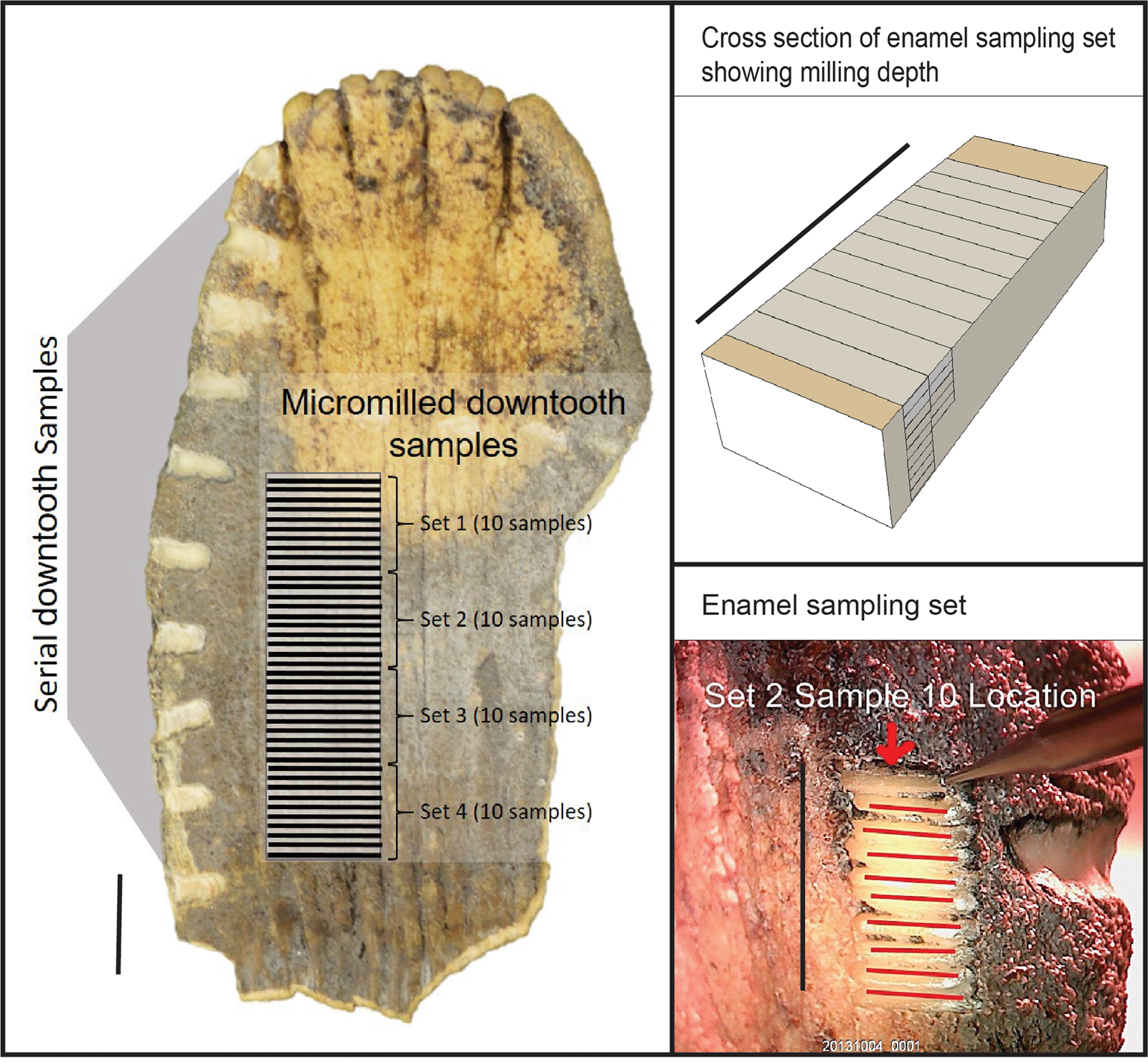
Figure 2. (color online) Schematic illustration of serial and microsampling strategies. Black bar = 1 cm.
All enamel powder samples were measured in a Finnigan Delta Plus XL mass spectrometer in continuous-flow mode connected to a gas bench with a CombiPAL autosampler at the Iowa State University Stable Isotope Laboratory, Department of Geological and Atmospheric Sciences. Reference standards (NBS-18, NBS-19) were used for isotopic corrections and to assign the data to the appropriate isotopic scale. Corrections were done using a regression method using NBS-18 and NBS-19. Isotope results are reported in per mil (‰). The long-term precision (at 1σ) of the mass spectrometer is ± 0.09‰ for δ18O and ± 0.06‰ for δ13C, respectively, and precision was not compromised with small carbonate samples (~150 μg). Both δ13C and δ18O are reported relative to VPDB.
Enamel δ13C results were corrected to -14.1‰ to approximate the δ13C of dietary input (δ13Cdiet) (Bryant and Froelich, Reference Bryant and Froelich1995).
Enamel δ18O results were converted from VPDB to Standard Mean Ocean Water (SMOW) using the equation:

The δ18O of enamel phosphate (δ18Op) for these samples was calculated from the δ18O of enamel carbonate (δ18Oc) following Fox and Fisher (Reference Fox and Fisher2001):

Estimates of body water δ18O (δ18Ow) were calculated following Daux et al. (Reference Daux, Lécuyer, Héran, Amiot, Simon, Fourel and Martineau2008):

The 87Sr/86Sr component of enamel bioapatite reflects changes in the geochemical makeup of the surface on which an animal grazed during tooth formation. In the serial-scale analyses, enamel powder samples were split from the light isotope samples described above and represent the same portions of mammoth teeth. Each ~5 mg sample of powder was leached in 500 μL 0.1 N acetic acid for four hours to remove diagenetic calcite and rinsed three times with deionized water (centrifuging between each rinse). In the micromilled series, small sample sizes prevented Sr analyses from being performed on the same samples as δ13C and δ18O analyses. Therefore, Sr from these growth series was analyzed opportunistically, or at the scale of one sample every 2 mm.
All enamel samples were then dissolved in 7.5 N HNO3 and the Sr eluted through ion-exchange columns filled with strontium-spec resin at the University of Kansas Isotope Geochemistry Laboratory. 87Sr/86Sr ratios were measured on a thermal ionization mass spectrometer, an automated VG Sector 54 eight-collector system with a 20-sample turret, at the University of Kansas Isotope Geochemistry Laboratory. Isotope ratios were adjusted to correspond to a value of 0.71250 on NBS-987 for 87Sr/86Sr. We also assumed a value of 86Sr/88Sr of 0.1194 to correct for fractionation.
The distribution of 87Sr/86Sr values in vegetation across the surface of the midcontinent is determined by the values of soil parent material. In a large part of this region, surface materials are composed of allochthonous Quaternary deposits such as loess, alluvium, and glacial debris. Therefore, continent-scale Sr isoscape models derived from bedrock or water (Bataille and Bowen, Reference Bataille and Bowen2012) are not ideal for understanding first-order variability in midwestern 87Sr/86Sr. For these reasons, Widga et al. (Reference Widga, Walker and Boehm2017b) proposed a Sr isoscape for the Midwest based on surface vegetation. At a regional scale, these trends in vegetation 87Sr/86Sr reflect the Quaternary history of the region and are consistent with other empirically derived patterns in Sr isotope distribution from the area (Slater et al., Reference Slater, Hedman and Emerson2014; Hedman et al., Reference Hedman, Slater, Fort, Emerson and Lambert2018). Sr isotope values in mammoth enamel are compared to a 87Sr/86Sr isoscape constructed from the combined datasets of Widga et al. (Reference Widga, Walker and Boehm2017b) and Hedman et al. (Reference Hedman, Brandon Curry, Johnson, Fullagar and Emerson2009, Reference Hedman, Slater, Fort, Emerson and Lambert2018).
RESULTS
The collagen of 54 mastodons and 22 mammoths was analyzed for δ13Ccoll and δ15Ncoll (Table 2). Three mastodons have 14C ages that place them beyond the range of radiocarbon dating, and the youngest mastodons date to the early part of the Younger Dryas, shortly before extinction. Despite being well represented prior to the LGM and during deglaciation (i.e., Oldest Dryas, Bølling, Allerød, Younger Dryas), this dataset lacks mastodons from the study region during the coldest parts of the LGM. Mammoths are present in this dataset from 40 ka until their extinction in the region during the late Allerød.
Table 2. Mastodon and mammoth collagen stable isotope values, by chronozone. δ13C values are reported as ‰ relative to VPDB. δ15N values are reported as ‰ relative to AIR.
There is a substantial amount of overlap in the δ13Ccoll and δ15Ncoll of mammoths and mastodons through the duration of the dataset (Fig. 3, Table 2). Both taxa show average δ13Ccoll values around -21‰, consistent with a diet dominated by C3 trees, shrubs, or cool-season grasses. This is broadly consistent with variable but shared diets during time periods when both taxa occupied the region. The average δ13Ccoll values for mammoths (-20.4‰; s.d. = 1.0) is similar to that for mastodons (-21.0‰; s.d. = 0.7). The average δ15Ncoll for mammoths (7.5‰; s.d. = 1.3) is elevated compared to mastodons (4.4‰; s.d. = 2.0).

Figure 3. Changes in midwestern proboscidean collagen δ13C and δ15N through time, showing mastodons (red circles), mammoths (blue circles), and glacial stadials (gray bars). Specimen age is from Supplementary Table 3. Stadial chronology is from Rasmussen et al. (Reference Rasmussen, Bigler, Blockley, Blunier, Buchardt, Clausen and Cvijanovic2014). (For interpretation of the references to color in this figure legend, the reader is referred to the web version of this article.)
However, dietary relationships between taxa are not static through time. Prior to the LGM, both δ13Ccoll and δ15Ncoll are significantly different between mammoths and mastodons (δ13C t-test; P = 0.013; δ15N t-test; P = 0.010). During the Oldest Dryas, the δ13Ccoll of both taxa is very similar, although δ15Ncoll between mammoths and mastodons remains distinct (t-test; P = 0.012). During the Allerød, δ13Ccoll and δ15Ncoll between taxa are indistinguishable.
The δ13Ccoll signature of mastodon diets changes little throughout the last 50 ka. Despite a noticeable absence of mastodon material during the height of the LGM, the only significant shift in the δ13Ccoll of mastodon diets occurs between the Bølling and the Allerød (t-test; P = 0.008).
Mastodon δ15Ncoll values fall clearly into two groups: those that date prior to the LGM, and those that postdate the LGM. Mastodon δ15Ncoll values are significantly higher in pre-LGM samples than in samples dating to the Younger Dryas (t-test; P = 0.010), Allerød (t-test; P = 0.017), and Bølling (t-test; P < 0.000). Of note is a group of mastodons that show lower δ15Ncoll values during the Oldest Dryas, Bølling, Allerød, and Younger Dryas, when the average δ15Ncoll values decrease to values <5‰. A similar shift is not evident in mammoths at this time.
Mammoth δ13Ccoll during MIS 3 is significantly different from mammoths dating to LGM II (t-test; P = 0.008) or the Oldest Dryas (t-test; P = 0.005). There are no significant differences in mammoth δ15Ncoll between different time periods.
All serial enamel series were between 9 and 16 cm in length and represent multiple years. Stable oxygen isotopes of three MIS 2 mammoths (Principia College, Brookings, Schaeffer) overlap significantly, while MIS 4 (234JS75) and MIS 5e (232JS77) mammoths from Jones Spring show elevated values indicative of warmer conditions (Fig. 4, Table 3). The variance in serially sampled MIS 2 mammoths (average amplitude = 2.5‰) was not significantly different from the series from Jones Spring, dating to MIS 4 (amplitude = 2.9‰) (F-test; P = 0.320). However, the MIS 5e mammoth from Jones Spring has a smaller amplitude (1.1‰) compared to the MIS 4 mammoth (F-test; P = 0.003) and the three MIS 2 mammoths (F-test; P < 0.000). Strontium isotope ratios of this animal indicate a home range on older, more weathered surfaces of the Ozarks throughout tooth formation, with a period of relatively elevated 87Sr/86Sr values also corresponding to low δ18O values.

Figure 4. (color online) Time series, serial enamel δ13C, δ18O, and 87Sr/86Sr.
Table 3. Summary of serial and microsampled Mammuthus tooth enamel: δ13C, δ18O, and 87Sr/86Sr.
Two mammoth teeth from Jones Spring were microsampled (Fig. 5). These specimens are from beds representative of MIS 4 and MIS 3 deposits.

Figure 5. (color online) Time series, microsampled enamel δ13C, δ18O, and 87Sr/86Sr. Both specimens are from Jones Spring, Hickory County, Missouri.
The MIS 3 molar (64JS73) shows regular negative excursions in δ18O values. These excursions are relatively short-lived and extreme. Considering the comparatively small analytical uncertainty (± 0.09‰), we interpret these data as reflecting seasonal changes in ingested water. This is consistent with δ18O in enamel series of other hypsodont mammals, such as bison and horses (Higgins and MacFadden, Reference Higgins and MacFadden2004; Feranec et al., Reference Feranec, Hadly and Paytan2009; Widga et al., Reference Widga, Walker and Stockli2010). Seasonal variation in enamel growth rate and maturation may account for the perceived short length of these periods. Maximum δ18O values in both mammoths are similar, however; the MIS 4 mammoth lacks these negative excursions and exhibits values that are more complacent through the length of the tooth. The δ13C series from both molars indicate these mammoths experienced a C4 diet throughout the year. However, deep dips in the δ18O series of the MIS 3 molar also correspond to at least two temporary peaks in the δ13C series.
The 87Sr/86Sr isotope series from both animals demonstrate an adherence to separate home ranges (Fig. 6). The MIS 4 mammoth shows values similar to bedrock units outcropping locally in central-western Missouri and neighboring areas of Kansas and Oklahoma. The MIS 3 mammoth, however, had a home range across rock units with much higher 87Sr/86Sr values. The home ranges for these animals do not overlap, despite their recovery from different strata within the same locality.

Figure 6. (color online) Mobility in mammoths from Jones Spring, Hickory County, Missouri. Hatched areas indicate the range of 87Sr/86Sr values from mammoth molar ridge-plates. One mammoth (305JS77) exhibits local values. Two separate mammoths (232JS77, 64JS73) exhibit Sr values, suggesting >200 km movement from the central core of the Ozark uplift. This implies movement over multiple years that is at least six times larger than the maximum home-range size documented for modern elephants in Etosha National Park, Namibia, Ngene et al. Reference Ngene, Okello, Mukeka, Muya, Njumbi and Isiche2017. Basemap isoscape data are from Widga et al. (Reference Widga, Walker and Boehm2017b) and Hedman et al. (Reference Hedman, Brandon Curry, Johnson, Fullagar and Emerson2009, Reference Hedman, Slater, Fort, Emerson and Lambert2018).
DISCUSSION
Despite overall similar isotopic values in mammoths and mastodons throughout the period of this study, underlying nuances are informative to regional changes in niche structure and climate. The absence of dated mastodons during the coldest parts of the LGM suggests that Mammut was, at least to some degree, sensitive to colder climates and adjusted its range accordingly.
Comparisons between coeval mammoths and mastodons indicate a gradual collapse of niche structure. Prior to MIS 2, δ13Ccoll and δ15Ncoll values between taxa were significantly different. By the end of the Allerød, mammoth and mastodon diets were isotopically indistinguishable.
Through time, there was no significant change in the δ13Ccoll of mastodons. Although average mammoth δ13Ccoll in the region during the latter part of the LGM was slightly more negative than in other time periods, this is not a marked shift and may be a function of decreased partial pressure of carbon dioxide during that time (Schubert and Jahren, Reference Schubert and Jahren2015). Globally, Siberian and European mammoths exhibit a similar range of δ13Ccoll values (Iacumin et al., Reference Iacumin, Di Matteo, Nikolaev and Kuznetsova2010; Szpak et al., Reference Szpak, Gröcke, Debruyne, MacPhee, Guthrie, Froese and Zazula2010; Arppe et al., Reference Arppe, Karhu, Vartanyan, Drucker, Etu-Sihvola and Bocherens2019; Schwartz-Narbonne et al., Reference Schwartz-Narbonne, Longstaffe, Kardynal, Druckenmiller, Hobson, Jass and Metcalfe2019).
In both taxa, mean δ15Ncoll decreases slightly throughout the sequence; however, the minimum δ15N values for mastodons during the Bølling, Allerød, and Younger Dryas are significantly lower than for earlier mastodons. The anomalously low values of these late mastodons are also shared with other published mastodon values in the Great Lakes region (Metcalfe et al., Reference Metcalfe, Longstaffe and Hodgins2013). They are also significantly lower than contemporary midwestern, Eurasian or Beringean mammoths (with some exceptions; see Drucker et al., Reference Drucker, Stevens, Germonpré, Sablin, Péan and Bocherens2018). The timing of these low mastodon δ15Ncoll values corresponds to regionally low δ15Ncoll values in the bone collagen of nonproboscidean taxa from European late Quaternary contexts (Richards and Hedges, Reference Richards and Hedges2003; Stevens et al., Reference Stevens, Jacobi, Street, Germonpre, Conard, Munzel and Hedges2008; Drucker et al., Reference Drucker, Bridault, Iacumin and Bocherens2009; Rabanus-Wallace et al., Reference Rabanus-Wallace, Wooller, Zazula, Shute, Jahren, Kosintsev and Burns2017), suggesting broad changes in global climate may have had cascading impacts in the nitrogen budget of local ecosystems.
Understanding in more detail how climate might have affected N cycling in midwestern ecosystems remains unclear. Flux in soil and plant N may be a function of plant-based N2 fixation (Shearer and Kohl, Reference Shearer, Kohl, Knowles and Blackburn1993), rooting depth (Schulze et al., Reference Schulze, Chapin and Gebauer1994), N loss related to climate factors (Handley and Raven, Reference Handley and Raven1992; Austin and Vitousek, Reference Austin and Vitousek1998), microbial activity, or mycorrhizal colonization (Michelsen et al., Reference Michelsen, Quarmby, Sleep and Jonasson1998; Hobbie et al., Reference Hobbie, Macko and Williams2000). Furthermore, the role of large herbivore populations in N flux may be significant (Frank et al., Reference Frank, David Evans and Tracy2004). In N-limited environments such as tundra, terrestrial plants may receive relatively more N from inorganic sources. Boreal forests like those of the Midwest during the Bølling and Allerød, however, exhibit relatively greater biological productivity, so plant shoots are more likely to take in volatized ammonia (low δ15N) from organic sources such as urea (Fujiyoshi et al., Reference Fujiyoshi, Sugimoto, Tsukuura, Kitayama, Lopez Caceres, Mijidsuren and Saraadanbazar2017).
At this time, it is difficult to distinguish which (if any) of these factors had an impact on late Quaternary mastodon δ15Ncoll values. Although there is a wide range in δ15Ncoll of mammoths and mastodons throughout the sequence, δ15Ncoll values below 5‰ are only present in mastodons during post-LGM deglaciation in the lower Great Lakes (39–43° latitude), throughout an area suggested to be vegetated by a disharmonious flora dominated by black ash and spruce (Gill et al., Reference Gill, Williams, Jackson, Lininger and Robinson2009; Gonzales and Grimm, Reference Gonzales and Grimm2009) (Fig. 7). The low δ15Ncoll values suggest that these mastodons occupied an undefined, local-scale dietary niche that was not shared by contemporary mammoths or by earlier mastodons. Previous research has suggested that the Bølling-Allerød may have been a time of high mastodon populations in the Great Lakes region (Widga et al., Reference Widga, Lengyel, Saunders, Hodgins, Walker and Wanamaker2017a). The concentration of mastodons around water sources may have had an impact on the δ15N of browsed plants owing to increased contributions of herbivore urea. Isotopically light plant shoots can occur with increased utilization of volatized NH4 from organic sources, including urea from herbivores.

Figure 7. Distribution of mastodons with associated δ15Ncoll <5‰ data (black circles) and δ15Ncoll >5‰ data (red circles) during the Bølling-Allerød. (For interpretation of the references to color in this figure legend, the reader is referred to the web version of this article.)
Life histories of midwestern mammoths
Through analyses of incremental growth structures in mammoths, such as molar enamel or tusk dentin, we can reconstruct longitudinal life histories that reflect the landscape experienced by an animal over multiple years. Late Pleistocene mammoths from the study region exhibit relatively consistent downtooth patterns in δ13C and δ18O. Similar bulk enamel isotope values in South Dakota, Wisconsin, and Illinois mammoths suggest access to broadly similar resources and relatively stable access to these resources across multiple years of the life of an individual (Fig. 4). Less negative δ13C and δ18O values in the last forming samples of the Schaeffer mammoth suggest a change in that animal's life history in the year before death. This change could be explained by local environmental changes resulting in nutritional stress.
Two mammoths from the Jones Spring site in southwest Missouri provide a pre–LGM perspective on landscapes that mammoths occupied (Fig. 4). A tooth-plate dating to MIS 5e from Jones Spring has less negative δ18O and δ13C values compared to the MIS 2 samples. This indicates warmer overall conditions and a diet that incorporated more C4 grasses throughout multiple years. Pollen from the same stratigraphic units further suggests that southwestern Missouri during MIS 5e was dominated by Pinus (no Picea) with a significant nonarboreal component (King, Reference King1973). Importantly, Sr isotopes from this tooth indicate that while it was forming, the animal was foraging across surfaces that are more radiogenic than local values. The nearest area with 87Sr/86Sr values >0.7140 is the central Ozark uplift to the east of Jones Spring (Fig. 6). The wide amplitude of δ18O values throughout the length of this tooth combined with the Sr isotope data indicating adherence to the central Ozark uplift suggest relatively broad shifts in annual water availability or that this animal utilized a variety of water sources, including surface sources and freshwater springs.
The MIS 4 molar from Jones Spring has δ18O values intermediate between the MIS 2 samples and the MIS 5e sample, along with δ13C values that indicate more C4 consumption than MIS 2 samples (Fig. 4). This mammoth occupied a cooler environment than the MIS 5e mammoth, but it was significantly warmer than that of the late Pleistocene mammoths in the MIS 2 group.
In the case of the two microsampled mammoths from Jones Spring, isotopic trends in each animal illustrate different life histories (Fig. 5). The MIS 4 mammoth occupied the western Ozarks, as indicated by 87Sr/86Sr values deposited throughout the development of the sampled portion of the tooth. It occupied a landscape where C4 vegetation was common, with mild winter temperatures. The MIS 3 mammoth occupied the central core of the Ozark uplift, as indicated by 87Sr/86Sr values deposited during the formation of the sampled tooth. However, between the cessation of enamel formation and death, this animal moved ~200 km to the western Ozarks, where it was preserved in the Jones Spring deposits. The δ18O series of this animal suggests greater seasonality during MIS 3 compared to MIS 5e, with deep negative excursions during the cold season. It also had a diet composed primarily of C4 vegetation.
These results suggest a broadly similar geographic scale of landscape use in late Quaternary mammoths in the Midwest to mammoths in the Great Plains and Florida (Hoppe et al., Reference Hoppe, Koch, Carlson and Webb1999; Hoppe, Reference Hoppe2004; Esker et al., Reference Esker, Forman, Widga, Walker and Andrew2019). Overall, mammoths from both regions do not engage in significant seasonal migrations but can move greater distances at annual to decadal timescales. Further, although δ13Ccoll values in mammoths clearly suggest a niche that at times included C3-rich diets in a region that was dominated by forest, not grasslands, both Jones Spring mammoths were mixed feeders, with C4 grasses making up a significant part of their diet. The individual life histories of these mammoths were highly variable, underscoring the need to control for individual mobility in stable isotope studies of large herbivore taxa.
Testing scenarios of late Pleistocene proboscidean population dynamics
Can this stable isotope dataset illuminate trends in late Proboscidean population dynamics during deglaciation in the Midwest? It is possible that the shift in δ15N represents the colonization of a novel ecological niche that also coincides with climate and vegetation changes at the beginning of the Bølling-Allerød. However, it is unclear what this niche might be. Stable isotopes alone do not adequately define this niche space, and further paleobotanical work is necessary. Drucker et al. (Reference Drucker, Stevens, Germonpré, Sablin, Péan and Bocherens2018) also noted anomalously low δ15N values in LGM mammoths from Mezyhrich in central Europe and attributed this pattern to a large, but unspecific, shift in dietary niche. This is counter-intuitive in warming landscapes of the Midwest, since boreal forests typically have increased amounts of N-fixing microbes relative to tundra environments, thus increasing the δ15N in forage overall.
Some studies have suggested that the growth rate of an individual is inversely correlated with δ15N (Warinner and Tuross, Reference Warinner and Tuross2010). This would be consistent with some scenarios of late Pleistocene mastodon population dynamics. Fisher (Reference Fisher and Haynes2009, Reference Fisher2018) suggests that predator pressure from Paleoindian groups who were megafaunal specialists would have caused mastodons to mature at a younger age. A decrease in the age at weaning would mean a shorter period of nursing-related elevated dietary δ15N in young mastodons. If this were the case, we would expect an overall decrease in δ15N of bone collagen in animals in their first and second decade of life. In our dataset, there is no significant change in maximum or mean δ15N in mastodon bone collagen, despite a subset of mastodons that have lower δ15N values. If predator pressure is contributing to faster maturation and shortening the time of nursing, then it is only occurring in some areas. However, even if this were the case in these areas, it is still uncertain what ecological processes might drive an increase in growth rate. Depending on local forage conditions experienced by an animal, an increase in growth rate may be caused by increased predator pressure (Fisher, Reference Fisher and Haynes2009) or a decrease in population density (Wolverton et al., Reference Wolverton, Lyman, Kennedy and La Point2009).
It is also possible that low δ15N values in post-LGM mastodons represent a systematic change in predator avoidance strategies among some mastodon populations (Fiedel et al., Reference Fiedel, Feranec, Marino and Driver2019). Mastodons may have been attracted to low δ15N areas such as marshes and wetlands as a response to new predators on the landscape (i.e., humans). However, taphonomic modification of late Pleistocene proboscidean materials by humans or other predators is extremely rare in this dataset (Widga et al., Reference Widga, Lengyel, Saunders, Hodgins, Walker and Wanamaker2017a), so we see this scenario as an unlikely driver of mastodon landscape use.
In times when populations are dense on the landscape (Widga et al., Reference Widga, Lengyel, Saunders, Hodgins, Walker and Wanamaker2017a) there may also be rapid, significant, and long-term changes to the N cycle. An influx of N via urea, as would be expected in high-density areas, would cause isotopically heavy plant roots and isotopically light shoots. Under intense grazing pressure, changes to N contributions change quickly from inorganic soil mineral N reservoirs to N from urea (McNaughton et al., Reference McNaughton, Ruess and Seagle1988; Knapp et al., Reference Knapp, Blair, Briggs, Collins, Hartnett, Johnson and Towne1999). Individuals with lower δ15Ncoll values during the Allerød lived in areas with high mastodon populations, which may have contributed to isotopically light forage (due to ammonia volitization; see Knapp et al., Reference Knapp, Blair, Briggs, Collins, Hartnett, Johnson and Towne1999). However, this scenario does not explain why this shift is absent in our mammoth data during this time.
CONCLUSIONS
Stable isotopes of proboscidean tissues in midwestern North America illustrate the variability inherent in modern paleoecological analyses. Traditional approaches to understanding animal diets and landscape use through morphology and a reliance on modern analogues is inadequate for understanding paleoecological changes in megafaunal populations or during times of rapid ecological change, such as the late Quaternary.
Stable isotopes from bone collagen of midwestern proboscideans suggest consistently C3-dominated diets over the last 50 ka. During the LGM, mammoth diets may have included C3 grasses, but the prevalence of C3 flora during the post-LGM period is likely due to a landscape shift to more forest (Gonzales and Grimm, Reference Gonzales and Grimm2009; Saunders et al., Reference Saunders, Grimm, Widga, Dennis Campbell, Curry, Grimley and Hanson2010), with grasses making up very little of the floral communities in the southern Great Lakes region.
Despite the strong C3-signal in mammoth and mastodon diets during this period, the range of dietary flexibility and the degree of overlap between these two taxa is striking. The isotopically defined dietary niche of mammoths and mastodons shows increasing overlap as they approach extinction. Niche overlap is also supported by assemblages where both taxa co-occur (Saunders et al., Reference Saunders, Grimm, Widga, Dennis Campbell, Curry, Grimley and Hanson2010; Widga et al., Reference Widga, Lengyel, Saunders, Hodgins, Walker and Wanamaker2017a). However, there are exceptions to this pattern, and some late mastodons exhibit low δ15N values that may indicate the evolution and occupation of a new dietary niche, physiological responses to late Pleistocene ecological changes, or some other process acting on late mastodon populations.
Further resolution of mammoth and mastodon life histories are gleaned from stable isotopes in tooth enamel. δ13C and δ18O generally track climate and landscape changes experienced during tooth formation. MIS 2 mammoths are broadly similar in their isotopic life histories and illustrate relative homogeneity of landscape conditions across the Midwest at this time. Microsampled mammoth molars from Jones Spring, Missouri, indicate a significant increase in MIS 3 seasonality compared to MIS 4. Finally, some mammoths in this study died >200 km from where they lived during the formation of sampled molars, suggesting that lifetime mobility patterns in mammoths could have a significant effect on presumed “local” stable isotope values.
ACKNOWLEDGMENTS
The study benefited from discussions with Paul Countryman, Eric Grimm, and Bonnie Styles, then at the Illinois State Museum; Rhiannon Stevens, at University College of London; and Matt G. Hill, at Iowa State University. Additional conversations with Don Esker and Matt Harrington greatly clarified micromilling methods, and Joseph Andrew, University of Kansas, assisted with Sr isotope analyses. Jeff Pigati and two anonymous reviewers provided invaluable feedback for strengthening the manuscript. This research was funded by National Science Foundation grants 1050638, 1049885, and 1050261, and the Illinois State Museum Society. Finally, we would like to acknowledge the collections managers and curators who assisted with access to the specimens in their care.
SUPPLEMENTARY MATERIAL
The supplementary material for this article can be found at https://doi.org/10.1017/qua.2020.85


