


1. Introduction
It is well-recognized that the primary goal of development policy is to improve the living standards and well-being of individuals and households in developing countries. There is an extensive literature in economics and other social sciences that has explored the relationship between socioeconomic status and household outcomes in developed countries, particularly child health [Fay et al. (Reference Fay, Leipziger, Wodon and Yepes2005), Ghuman et al. (Reference Ghuman, Behrman, Borja, Gultiano and King2005), Boyle et al. (Reference Boyle, Racine, Georgiades, Snelling, Hong, Omariba and Rao-Melacini2006), Paxson and Schady (Reference Paxson and Schady2007), Wehby and McCarthy (Reference Wehby and McCarthy2013), Rubio-Codina et al. (Reference Rubio-Codina, Attanasio, Meghir, Varela and Grantham-McGregor2015)]. Understanding the relationship between socioeconomic status and child health is of vital importance since poor health in childhood is associated with lower educational attainment, inferior labor market opportunities, and worse health outcomes later in life [Currie (Reference Currie2009)]. Public policies have the potential to address such issues through early intervention implemented to reduce inequalities in child health and this may further help mitigate the intergenerational transmission of poverty, which is of utmost concern for developing countries. Our paper makes a unique contribution to this literature by using household consumption expenditure as a measure of socioeconomic status to examine its effect on child health in Vietnam.
Research has shown that improving child health outcomes in low-income countries is challenging because of nutrition problems and poor health care services [Nguyen (Reference Nguyen2016)]. Also, there is a considerable disparity in the health of children living in poor households relative to those from wealthier households, especially in rural areas. Therefore, it is reasonable to hypothesize that the social gradient in child health will be steeper in developing countries. Nonetheless, very few studies to date have investigated this relationship in developing countries [exceptions include Cameron and Williams (Reference Cameron and Williams2009), Miller and Urdinola (Reference Miller and Urdinola2010), Fichera and Savage (Reference Fichera and Savage2015)].Footnote 1 The main impediment to conducting such studies in developing countries is the lack of reliable data.
A range of measures have been used to capture individuals' or households' socioeconomic status, including income, wealth, education, employment, and consumption [Montgomery et al. (Reference Montgomery, Gragnolati, Burke and Paredes2000), Australian Bureau of Statistics (2011)]. Most existing studies that investigate the health–wealth nexus or the income–health gradient have used an index of wealth or income as a measure of socioeconomic status [Sastry (Reference Sastry2004), Fay et al. (Reference Fay, Leipziger, Wodon and Yepes2005), Filmer (Reference Filmer2005), Currie et al. (Reference Currie, Shields and Wheatley Price2007), Khanam et al. (Reference Khanam, Nghiem and Connelly2009)]. While household income is frequently available in household surveys in developed countries, it is not a common feature in their counterpart developing countries because of lack of reliability, and the cost and time involved in data collection. Large income fluctuations and in-kind income, which are common features in developing countries especially where agriculture is the main source of employment, can potentially bias income reporting [see, e.g., Montgomery et al. (Reference Montgomery, Gragnolati, Burke and Paredes2000), Rutstein and Johnson (Reference Rutstein and Johnson2004)]. The wealth index, on the other hand, has gained popularity in developing countries in recent years given that they are calculated using easy-to-collect data on household ownership of selected durable assets, such as a car, refrigerator, television or bicycle; materials used for housing construction; and types of water access and sanitation facilities [Rutstein and Johnson (Reference Rutstein and Johnson2004), Howe et al. (Reference Howe, Hargreaves, Gabrysch and Huttly2009)]. Yet, there are several potential limitations with the use of a wealth index as a measure of socioeconomic status or living standards [Howe et al. (Reference Howe, Hargreaves, Gabrysch and Huttly2009), Filmer and Scott (Reference Filmer and Scott2012)]. Firstly, the set of indicators used to construct the wealth index are chosen on the basis of availability and convenience rather than on theoretical grounds [Gwatkin et al. (Reference Gwatkin, Rutstein, Johnson, Suliman, Wagstaff and Amouzou2007)]. Secondly, access to water or electricity, a main component of the wealth index construction, is often a community rather than a household-level characteristic [Knodel and Wongsith (Reference Knodel and Wongsith1991)], making it less likely to be a unique and relevant indicator of a household's standard of living. Lastly, a household's ownership of selected items could result from preference rather than financial constraints and does not necessarily reflect living standards [Perry (Reference Perry2002)].
In the absence of household income in our dataset and the limitations of the wealth index discussed above, we use household expenditure as a measure of living standards, which makes an important and unique contribution to the literature. We advocate this measure on the following two grounds. Firstly, while the health–income relationship is well documented, the mechanisms via which income affects child health, in which household consumption arguably plays a crucial role, remain unclear. Our study serves to shed light on this pathway. Secondly, we argue that household expenditure can by itself be a better measure of standard of living than household income. It is common for households in developing countries to draw their income from multiple sources, and as mentioned before, these sources are highly variable from season to season, especially in countries which rely largely on agriculture. As such, household income will be measured accurately only if it takes into account the primary and secondary employment and nature of payment for each adult household member [Montgomery et al. (Reference Montgomery, Gragnolati, Burke and Paredes2000), Rutstein and Johnson (Reference Rutstein and Johnson2004)]. In contrast, expenditure is considered more stable than income as households tend to “smooth” their consumption by borrowing or saving in times of temporary income fluctuations [Howe et al. (Reference Howe, Hargreaves, Gabrysch and Huttly2009)]. For example, some studies have found significant measurement error in reported income, to the extent that expenditures reported by families with low income are often multiples of their reported incomes [Rogers and Gray (Reference Rogers and Gray1994), Sabelhaus and Groen (Reference Sabelhaus and Groen2000)].
The data we use in this paper comes from the Young Lives Project, a longitudinal study administered by the University of Oxford. This dataset has been used extensively in the literature [Krishna et al. (Reference Krishna, Fink, Berkman and Subramanian2016), López Boo (Reference López Boo2016), Humphries et al. (Reference Humphries, Dearden, Crookston, Woldehanna, Penny and Behrman2017)]. Vietnam provides an interesting case to examine the relationship between household socioeconomic status and child health. Child health is a significant issue in Vietnam with more than 23% of children less than 5 years old reported as under normal height, and about 12% of children reported under-weight [Nguyen (Reference Nguyen2016)]. Furthermore, the incidence of underweight children and stunted growth is higher in lower socioeconomic households. Hence, there is an urgent need for intervention policies in Vietnam to effectively tackle such children's health issues. While the government has expanded its universal health insurance coverage to children from vulnerable households by giving them free access to health services, there is no evidence of any health improvement in this population [Nguyen (Reference Nguyen2016)].
One significant concern in the analysis of child health and socioeconomic measures such as income, and which also applies to expenditure, is the endogeneity which could arise from two sources. Firstly, poor households are less likely to be able to provide adequate consumption and healthcare services to their children, but, in turn, poor child health may reduce parental earnings [Currie (Reference Currie2009)], thereby resulting in reverse causality. Secondly, both child health and income are determined by unobserved factors, such as parents' time preferences [Fichera and Savage (Reference Fichera and Savage2015)] or poor genetics [Burgess et al. (Reference Burgess, Propper and Rigg2004)], resulting in omitted variable bias. While the issues of endogeneity or spurious relationship have been discussed in the relevant literature, none of the early studies has explicitly dealt with it. More recent studies have addressed endogeneity using the generalized method of moments (GMM) [Khanam et al. (Reference Khanam, Nghiem and Connelly2009)]; and the Instrumental Variable (IV) approach [Doyle et al. (Reference Doyle, Harmon and Walker2007), Kuehnle (Reference Kuehnle2014)]. The GMM approach, which uses lagged variables of health, requires a relatively long panel of data on child health and related variables, which is often not available in developing countries. The IV approach relies heavily on valid instruments for the endogenous variable. To examine the impact of household expenditure on child health, we use the two-stage (2SLS) approach and we adopt the IV approach to deal with the endogeneity of expenditure and exploit two instruments, namely the unemployment rate and rainfall.
In terms of health measures, we use a range of health indicators, namely, body mass index (BMI), BMI-for-age Z-score (BMI-Z) and Height-for-age Z-score (HAZ), with height representing the long-run nutritional and health status of the child and BMI, being regarded as more of a short-run health metric. A Z-score is a child's BMI (or height) expressed as a number of standard deviations from the mean BMI (height) of children of the same age and gender in a healthy population. The reference population used in the survey is the US population, as recommended by the World Health Organization (WHO). In comparison to self-reported health that has been used in previous studies [e.g., Case et al. (Reference Case, Lubotsky and Paxson2002), Apouey and Geoffard (Reference Apouey and Geoffard2013), Kuehnle (Reference Kuehnle2014)], there is less subjectivity in the reporting of anthropometric indicators. Nonetheless, we also use self-reported health to test the robustness of our findings. Our main results suggest a strong positive relationship between household expenditure and child physical health. Specifically, we find that a 10% increase in total household expenditure will result in a weight gain of 213–541 g in a “typical” child, with the findings being consistent across different age groups.
2. Econometric framework
As a reference case, we start with a model in which household expenditure is treated as exogenous. The impact on child health is therefore estimated as follows:

where Y it is a vector of health indicators of child i at time t, specifically (1) BMI, (2) BMI-Z, and (3) HAZ. We use two alternative measures of household expenditure (E it) of child i at time t: household total expenditure and household food expenditure per capita (in logs). C it is a vector of child characteristics such as age and gender. Other control variables include parental characteristics (P it) such as education and age; and household characteristics (H it) such as household size and geographical location.Footnote 2
As discussed above, a potential source of bias in equation (1) arises from the potential reverse causality between household expenditure (E it) and child health (Y it). For example, poor households are less likely to provide adequate consumption and healthcare services to their children but, in turn, children with poor health may require greater parental care, thus resulting in a reduction in parental labor supply and household consumption. Another potential source of bias results from omitted variables. For example, parental genetics and attitudes toward children may be highly correlated with both household income and child health [Currie (Reference Currie2009), Fichera and Savage (Reference Fichera and Savage2015)]. To address such endogeneity issues, an IV approach is adopted. Specifically, we estimate:


where Z it is the instrumental variable for household expenditure in the first stage of the regression. The simultaneous equations (2) and (3) are then estimated using the 2SLS approach.Footnote 3
We have identified two potential instruments for household expenditure, the unemployment rate and rainfall deviation, which have been explored in the broader literature. Given that the selection of instruments is an area which is always open to debate, to explore the robustness of our findings, we use both as alternative instruments for household expenditure.Footnote 4
Firstly, we follow Kuehnle (Reference Kuehnle2014), who suggests using the local unemployment rate as an instrument for income. The rationale is that areas with a high unemployment rate are often associated with lower job opportunities, thereby affecting household income directly. This is also applicable in the context of developing countries and rural areas where agriculture is the main activity. For example, while fewer economic opportunities in rural areas may not directly impact on farm households, there is an indirect effect through reduced demand for agricultural products. However, using the unemployment rate as an instrument requires the assumption that children do not contribute to household income, which may not be the case for developing countries where children often participate in paid work or family businesses [Trinh (Reference Trinh2020)]. In this context, areas with a higher unemployment rate are likely to have lower proportions of child labor, resulting in better health outcomes [Doyle et al. (Reference Doyle, Harmon and Walker2007), Sim et al. (Reference Sim, Suryadarma and Suryahadi2017)]. In order to deal with the possible association between unemployment and child labor, we exclude children who are engaged in any type of work (paid or unpaid).Footnote 5 Another concern is the direct impact of unemployment on child health via parent's debilitating mental health. However, with an extended family setup in Vietnam, especially in rural areas, where children are often looked after by other family members, financial distress is arguably the most likely pathway through which unemployment impacts child health.
Our second instrument, which is rainfall deviation, relates to a more recent literature [Case et al. (Reference Case, Lubotsky and Paxson2002), Apouey and Geoffard (Reference Apouey and Geoffard2013), Kuehnle (Reference Kuehnle2014), Fichera and Savage (Reference Fichera and Savage2015)]. The core idea is that climatic shocks impact on agricultural production and, consequently, farmers' living standards [Mendelsohn et al. (Reference Mendelsohn, Nordhaus and Shaw1994), Deschênes and Greenstone (Reference Deschênes and Greenstone2007), Trinh (Reference Trinh2018)]. Adverse weather conditions are likely to cause crop failure, thereby impacting on household income and expenditure. However, it is important to acknowledge that weather conditions can have a direct impact on child health outcomes. For example, it has been argued that adverse weather shocks, such as drought or flood, may directly contribute to the incidence or spread of diseases, such as malaria or poor sanitation [Thai and Falaris (Reference Thai and Falaris2014), Cornwell and Inder (Reference Cornwell and Inder2015), Lohmann and Lechtenfeld (Reference Lohmann and Lechtenfeld2015)]. Weather shocks are also found to impact on the parental allocation of time or household migration, thereby affecting child health outcomes [Connolly (Reference Connolly2008), Gröger and Zylberberg (Reference Gröger and Zylberberg2016)]. To address such concerns, instead of using weather shocks or short-term changes in rainfall, we use the long-term change in precipitation, as measured by the deviation of actual rainfall from historical levels. This helps mitigate any possible direct association between environmental factors and child health.Footnote 6 The link between rainfall deviation and expenditure can operate in both directions. A higher deviation of rainfall may improve agricultural activities by increasing water supply, but it may also destroy crop production by providing conditions for insects to develop. As such, which mechanism dominates is not important in our analysis, as long as it has a positive or negative correlation with household expenditure.Footnote 7
3. Data
This paper uses panel data which come from the Young Lives Project, administrated by the Department of International Development at the University of Oxford. This is a 15-year longitudinal study of childhood poverty covering the lives of children in four developing countries: Ethiopia, India, Peru, and Vietnam. Using four surveys, the project tracks more than 12,000 children in the four countries from 2002 to 2014, with a roughly equal number of boys and girls. The overall objective of the project is to promote a broad-based and multi-dimensional understanding of child development, poverty, and welfare in these countries, and in turn, to inform the development of policies that will reduce poverty.
In Vietnam, the survey follows 3,000 children in five provinces: Phu Yen, Ben Tre, Lao Cai, Hung Yen, and the city of Da Nang. There are 2,000 children born in 2001–2002 (the younger cohort), and 1,000 born in 1994–1995 (the older cohort). By using a sentinel sampling approach, the Young Lives data mainly focus on poor households in rural areas. In each province, four communes were selected for interview.Footnote 8 Of the four selected, two communes were poor, one was average, and one was above average. The city of Da Nang, which is the only urban area chosen for the survey, is less developed than other large cities such as Hanoi and Ho Chi Minh City. We use an unbalanced panel over the period 2006–2014 (e.g., three survey rounds),Footnote 9 where the total number of observations is 5,515, comprising 2,375 children. The percentage of children present in all three surveys is 50%.Footnote 10
Our focus on Vietnam relates to the fact that, in addition to child health being a significant issue in Vietnam, compared to the other three countries in the Young Lives Project, Vietnam is a unique case study with detailed data on child health available in all rounds. The survey also includes household information such as household expenditure and food consumption; the holding of land, durable good ownership, and productive assets; families' financial situation; and a range of demographic characteristics.
Although the focus in the child health and wealth and child health and income gradient literatures has largely been on self-assessed health measures and morbidity, one widely used and more objective measure of child physical health used in other areas of economics is BMI, which is derived from the current height and weight of children in each round. However, a shortcoming of using BMI is its sensitivity to factors such as age, sex, and region [Beegle et al. (Reference Beegle, Dehejia and Gatti2009)]. This study therefore employs two other standardized measures of child anthropometry, which are constructed using the WHO guidelines: BMI-Z and HAZ [WHO (2010)].Footnote 11 The BMI-Z, also called BMI standard deviation scores, is a measure of relative weight adjusted for child age and sex, while the HAZ measures the child's standardized height adjusted for age and sex. Figure 1 plots the frequency distribution of children's BMI. The average BMI is 15.8; approximately 20% of children have a BMI lower than 15 and are thus considered underweight according to the WHO guidelines [WHO (2010)]. Conversely, only a very small percentage of children are overweight or obese (BMI of 25 or more). Given such a distribution, an increasing BMI can be considered as a measure of better health.Footnote 12 The Young Lives Project also provides information on child health reported by the biological mother. However, given the subjective nature of such information, we do not use this measure of health in our main analysis as it can potentially bias our findings [Currie (Reference Currie2009), Khanam et al. (Reference Khanam, Nghiem and Connelly2009)]. We have, however, explored the robustness of our findings to using this measure, as discussed further below.

Figure 1. Histogram of BMI for Vietnamese children.
Source: Authors' calculation using Young Lives data.
The two key independent variables we use as measures of living standards in our analysis are total expenditure and food expenditure per capita, measured in thousand VND. Both expenditure variables are deflated for inflation using the 2006 constant price. In terms of the explanatory variables, we include child characteristics (age and gender), parental characteristics (the father's and mother's age and years of education), and household characteristics (household size and an indicator of whether the child lives in a rural area). The set of explanatory variables ties in with that commonly used in studies conducted in developing countries [Thai and Falaris (Reference Thai and Falaris2014), Fichera and Savage (Reference Fichera and Savage2015), Mulmi et al. (Reference Mulmi, Block, Shively and Masters2016)].
Finally, the two instruments, the unemployment rate and rainfall deviation, are obtained from separate sources. Province-level unemployment rates, used to measure the proportion of unemployed people in the labor force in each period, are obtained from the annual Vietnam Statistical Handbook.Footnote 13 The rainfall data are derived from the monthly precipitation of Gridded Monthly Time Series (Version 4.01) dataset (GMTS), developed by the Centre for Climatic Research, University of Delaware. This dataset provides global historical estimates of rainfall for a grid of 0.5 degree by 0.5 degree of latitude and longitude, where the grid nodes are centered on 0.25 degree. Each grid, thus, covers an area of 50 km2. We then follow Trinh (Reference Trinh2018) and use the administrative map of Vietnam to determine the longitude and latitude for each province. These rainfall data are then matched with the household data in Young Lives using the four closest grid points in the GMTS dataset and the month of interview. In order to reflect the long-term impact of weather conditions, precipitation data are collected over a 65-year period (1950–2014) to obtain a historical average. We then define rainfall deviation as the difference between the actual rainfall (averaged over a 12-month period prior to interview date) and the historical average rainfall.
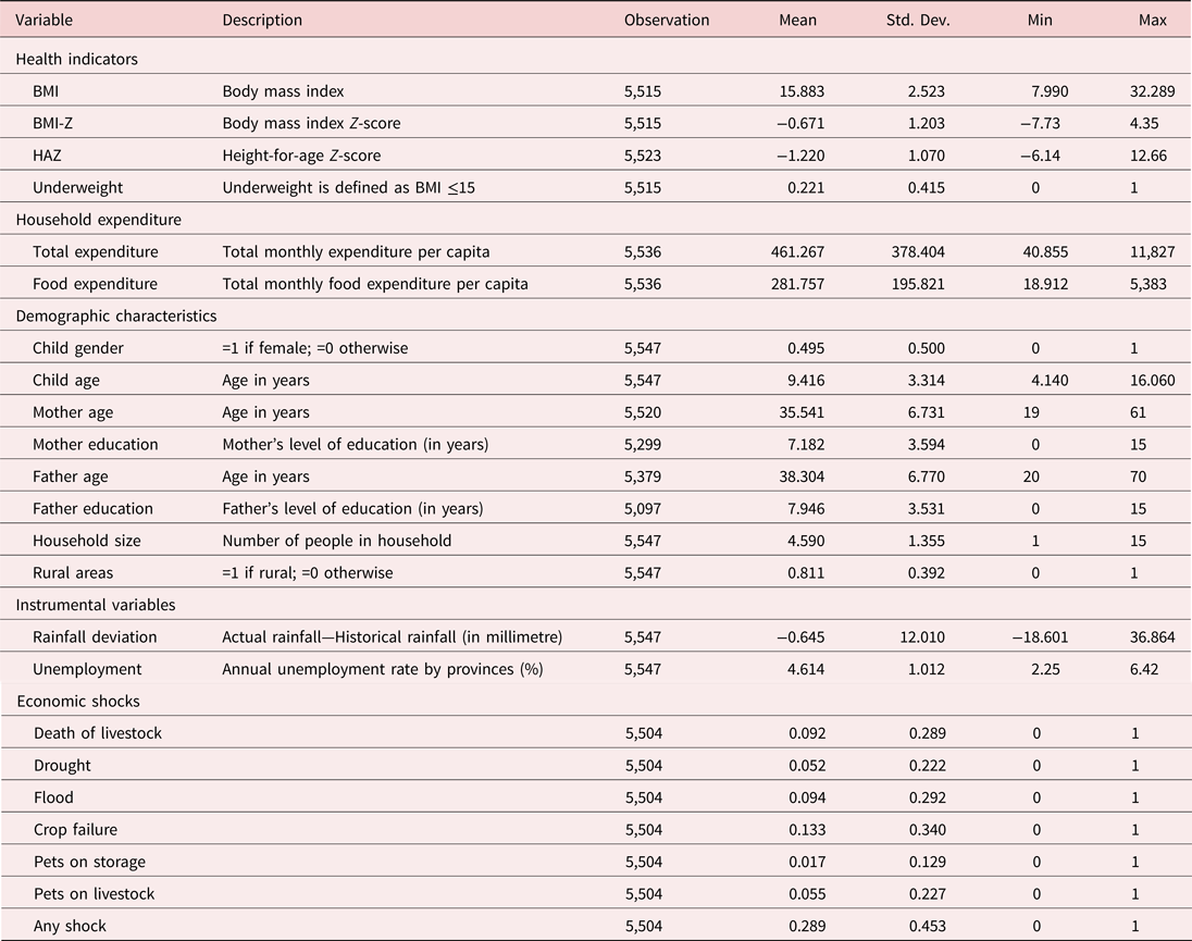
Table 1 provides summary statistics for all variables used in this study. The average BMI of children in the sample is 15.8. On average, households' consumption expenditure is 461,000 VND and their average food expenditure is 282,000 VND. The average number of years of education for fathers and mothers are approximately 8 and 7, respectively. Finally, more than 80% of households live in rural areas, and the average household size is 4.6.
Table 1. Summary statistics
As a precursor to the econometric analysis, in Figure 2, we examine the relationship between household expenditure and health, based on the observed data. Four health levels are constructed using the 25th, 50th, 75th, and 100th percentiles of BMI-Z and the sample is also split into two age groups: 4–9 and 10–16 years. The graph suggests a positive correlation between the two measures of expenditure and child health. The results are consistent across the two age groups.

Figure 2. Household expenditure and child health.
Notes: Four levels of child health are constructed using BMI-Z: Level 1—BMI-Z≤25th percentile, Level 2—25th percentile<BMI-Z≤50th percentile, Level 3—50th percentile<BMI-Z≤75th percentile, and Level 4—BMI-Z>75th percentile.
Source: Authors' calculation using Young Lives data.
4. Results
4.1 Main findings
As a starting point, we estimate equation (1) using the Ordinary Least Squares (OLS) approach on a pooled sample, treating expenditure as exogenous and using province fixed effects to account for differences in geographic characteristics across provinces. The results are presented in Table 2. The first set of results in columns 1–3 relates to total expenditure used as a measure of living standards and columns 4–6 are estimated using food expenditure. Both sets of results indicate a strong correlation between household expenditure and child physical health.Footnote 14 For instance, 1% higher total expenditure and food expenditure is associated with 0.0053 and 0.0038 higher BMI, respectively.
Table 2. Household expenditure and child health: expenditure as exogenous
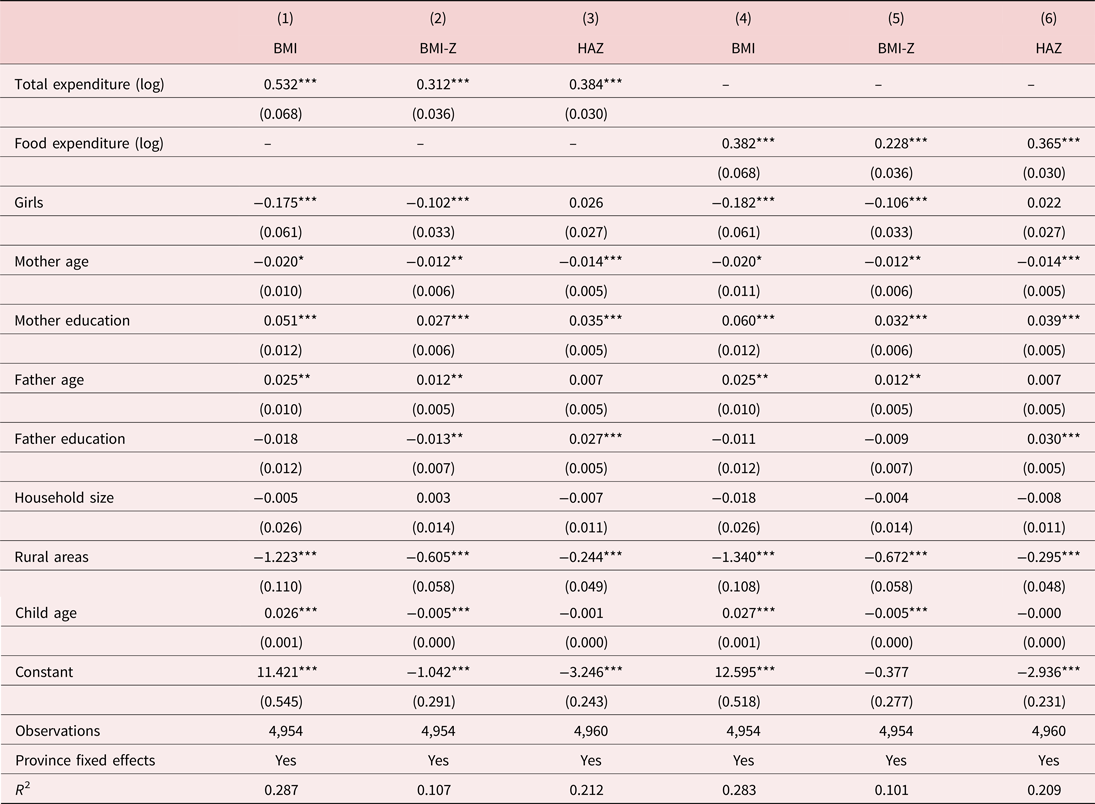
Notes: Estimated using OLS; robust standard errors in parentheses.
***p < 0.01, **p < 0.05, *p < 0.1.
Next, we employ the IV approach to further examine the relationship between household expenditure and child health.Footnote 15 This allows us to purge the correlation of household expenditure with the error term in equation (1) and to isolate the policy-driven effect of household expenditure on child health. From a policy perspective, these results inform health specialists about the likely impact of a food subsidy or cash transfer program on children's health.
We start by investigating the validity and strength of the two instruments, the unemployment rate and rainfall deviations. For an instrument to be valid, it must satisfy two conditions: firstly, it must have a statistically significant relationship with household expenditure; and, secondly, it needs to be uncorrelated with the residuals in equation (1). While the first condition is straightforward to test, the second condition (the exclusion restriction) cannot be tested, particularly if the model is just identified. However, as argued in the previous section, the two instruments are unlikely to have a direct effect on the child health outcomes. Table 3 shows a strong significant correlation between household expenditure and the two alternative instruments in the first-stage estimation (see the first row under panels A and B). As expected, a higher unemployment rate is associated with lower total and food expenditure, while a higher deviation of rainfall results in higher total and food expenditure.
Table 3. Instrument performance
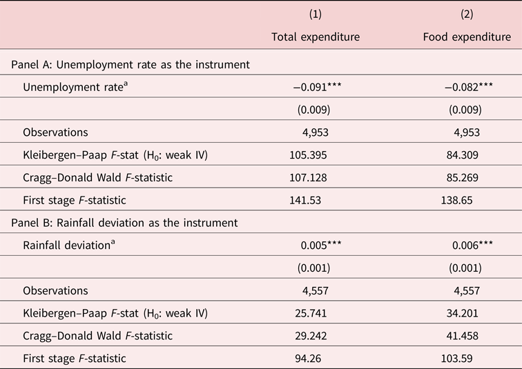
Notes: Robust standard errors in parentheses.
a Partial effects from first stage of the 2SLS. Other control variables include child gender and age, mother's age and education, father's age and education, household size, and an indicator for rural areas. The critical value of the F-test from Stock and Yogo (Reference Stock and Yogo2002) is 16.38.
***p < 0.01, **p < 0.05, *p < 0.1.
We examine the strength of the instruments using the critical values tabulated by Stock and Yogo (Reference Stock and Yogo2002). We test for weak instruments using the first stage F-statistic (the rule of thumb is that this statistic is greater than 10), the Kleibergen–Paap Wald F-statistic and the Cragg–Donald Wald F-statistic. Under the null hypothesis, we assume that the instrument is weak. The critical value of 16.38 [Stock and Yogo (Reference Stock and Yogo2002)] implies a rejection of the null hypothesis for both the unemployment rate (Panel A) and rainfall deviation (Panel B) using all three statistics, hence endorsing the strength of the selected instruments.Footnote 16
We now move on to discuss our main results, which are shown in Table 4, with the model estimated using the unemployment rate (Panel A) and rainfall deviation (Panel B), and province fixed effects controlled for in all the regressions. The findings are generally consistent across the two empirical approaches, indicating a strong association between household expenditure and the child health outcomes, irrespective of the instruments used. This is explained by the fact that households with higher expenditure or higher living standards can consume better health and non-health inputs, as well as live in healthier environments. Higher income can also translate into an increase in the opportunity cost of time spent on health-promoting activities, especially by the mother [Miller and Urdinola (Reference Miller and Urdinola2010), Stoklosa et al. (Reference Stoklosa, Shuval, Drope, Tchernis, Pachucki, Yaroch and Harding2018)]. For example, important determinants of child health, such as, preparing nutritious food, bringing water from distant sources and travelling long distances to access health facilities, require a large amount of time [Miller and Urdinola (Reference Miller and Urdinola2010)]. Consumption expenditure can also be considered as a pathway through which income affects children's health as higher expenditure could result into better health care and nutrition. Our findings are consistent with this hypothesis.
Table 4. Household expenditure and child health: second stage of two-stage least squares estimation (2SLS)

Notes: Robust standard errors in parentheses.
***p < 0.01, **p < 0.05, *p < 0.1.
From Table 4, using the unemployment rate as an instrument, it is apparent that a 1% increase in total expenditure (food expenditure) is associated with a 0.013 (0.015) increase in BMI. With rainfall deviation as an instrument, the corresponding increase in BMI is of the order of 0.033 (0.028). While these effects may appear small, if we translate them into a change in weight for a “typical” child in our sample (i.e., at the mean values of all the explanatory variables), a 10% increase in total expenditure, for example, will result in a weight gain of 213 (541) grams based on the two partial effects of 0.013 and 0.033 from Panels A and B, respectively.Footnote 17 The results are generally consistent across the BMI-Z and HAZ measures providing additional support for the robustness of our findings. Specifically, we find that a 10% increase in, for example, food expenditure is associated with increases of 0.10 and 0.23 of a standard deviation in BMI and height, respectively. As noted earlier, relative to BMI representing the short-run health status of the child, height captures long-term, cumulative effects of poor nutrition, as it affects child development, particularly at younger ages. As such, our results indicate the existence of both long-run and short-run effects of expenditure on child health. We also estimate the models by clustering standard errors at province and commune levels and the results are generally consistent.Footnote 18
Clearly, the marginal effects of both expenditure variables in the IV model are larger than the respective OLS effects in Table 2, where we do not take account of potential reverse causality and the presence of unobserved heterogeneity. The negative bias in the OLS estimates could result from unobserved parental work choices (such as a preference to stay at home to provide better care to their children), which would be positively related to child health but negatively correlated to income and household consumption. Similarly, extended family set-ups could be negatively related to expenditure but could impact positively on child health. These results conform to prior studies that have found a larger IV estimate of income gradient relative to OLS [Doyle et al. (Reference Doyle, Harmon and Walker2007), Kuehnle (Reference Kuehnle2014), Fichera and Savage (Reference Fichera and Savage2015)]. For example, Kuehnle (Reference Kuehnle2014) finds that the IV estimate of the effect of income on the probability of a child being in poor health is four times larger than the OLS estimate.
Although our main interest lies in the relationship between household expenditure and child health, the coefficients on the other control variables provide some interesting results. For example, girls are more likely to have negative health outcomes compared to boys. Also, children living in urban areas with better access to healthcare services are more likely to have better physical health than those living in rural areas.Footnote 19 Interestingly, we find mixed evidence of the role of parental education on child health. The results mostly indicate a positive and significant relationship between mothers' education and child health, which could be explained by an accumulation of healthcare knowledge. However, in almost all estimations, we find a negative association between the father's education and child health. One likely reason could be the presence of multicollinearity between the mother's and father's education. We further explore this issue using alternative specifications. Firstly, we remove the mother's education from the models and find that the OLS estimate of the effect of the father's education becomes positive and significant. The IV estimate however remains negative but becomes statistically insignificant. Next, we estimate the models removing the father's education from the specification. We find that in all cases our main results remain essentially unchanged, lending confidence to our earlier results.Footnote 20
As a further test of the robustness of our results, we estimate the model with self-assessed health, which is a categorical variable defined as 1 for poor/very poor health, 2 for average health, and 3 for good health. We use the Conditional mixed-process (CMP) modeling approach, suggested by Roodman (Reference Roodman2011), to estimate equation (2) (an Ordered Probit specification) and equation (3) as a system with correlated error terms. Our results, presented in Table 5, are consistent with the previous findings. Both total expenditure and food expenditure have statistically significant effects on child health. This lends further support to the instruments we have used in the study.
Table 5. Household expenditure and child self-reported health

Notes: Robust standard errors in parentheses. Dependent variable is a categorical variable defined as 1 for poor/very poor health, 2 for average health, and 3 for good health. System of Ordered Probit and linear regression estimated using CMP. Other control variables include child gender and age, mother's age and education, father's age and education, household size, and an indicator for rural areas.
***p < 0.01, **p < 0.05, *p < 0.1.
We further explore the robustness of our results by estimating the health–expenditure relationship across two different age groups. This is motivated from the income–health gradient literature, which shows heterogeneous results across age groups. Some studies, particularly in developed countries, have found the relationship between child health and household income to be stronger for older children [e.g., Currie and Stabile (Reference Currie and Stabile2002), Burgess et al. (Reference Burgess, Propper and Rigg2004)]. In contrast, Cameron and Williams (Reference Cameron and Williams2009) did not find that the impact of income varies with age in Indonesia. Since previous studies have not established any systematic construct of age groups, we split our sample into: children aged from 4 to 9 years, and children aged from 10 to 16 years. The criteria we use here is that children move from primary to secondary education at the age of 10 in Vietnam.Footnote 21 The main results are presented in Table 6. Overall, we find a consistent effect of household expenditure on child health across the two age groups. For example, a 1% increase in total expenditure results in an increase in BMI of 0.021 (0.011) for the 4–9 (10–16) years old children (Panel A) when we instrument expenditure using unemployment, and of 0.041 (0.010) (Panel B) when we instrument expenditure using rainfall. However, given the small sample sizes, the results should be interpreted with caution.
Table 6. Household expenditure and child health by age-groups

Notes: Robust standard errors in parentheses. Estimated using 2SLS. Results of first stage are not shown. Other control variables include child gender and age, mother's age and education, father's age and education, household size, and an indicator for rural areas.
***p < 0.01, **p < 0.05, *p < 0.1.
Finally, in order to provide some further insights on the magnitude of the effects of household expenditure on child health, we estimate the effect of total expenditure and food expenditure on the probability that a child is underweight.Footnote 22 Specifically, we estimate a Probit model with expenditure as an endogenous regressor, where our dependent variable is now defined as U it = 1[δ 0 + δ 1I it + δ 2C it + δ 3P it + δ 4H it + w it] > 0 and U it is a binary indicator for whether a child is underweight at time t. Table 7 presents the results. The marginal effects of total expenditure and food expenditure (shown in brackets) are both statistically significant at the 1% level of significance. The findings indicate that a 1% rise in total (food) expenditure is associated with a 0.367 (0.300) decrease in the probability that a child will be underweight (using the unemployment rate as an instrument).
Table 7. Household expenditure and underweight children: IV-Probit model

Notes: Robust standard errors in parentheses. Marginal effects are shown in brackets. Results of the first stage are not shown. Other control variables include child gender and age, mother's age and education, father's age and education, household size, and an indicator for rural areas. Columns (1) and (3) use unemployment rate as an instrument, columns (2) and (4) use rainfall deviation as an instrument.
***p < 0.01, **p < 0.05, *p < 0.1.
4.2 Economic shocks and child health
In this section, we investigate the impact of adverse economic shocks on children's health. Specifically, we examine whether there are any differential effects of these shocks by socioeconomic status such that the shocks have a larger impact on children with lower household expenditure. Several studies have examined the impact of economic shocks on a range of child outcomes such as education, nutrition, and health [Jacoby and Skoufias (Reference Jacoby and Skoufias1997), Jensen (Reference Jensen2000), Duryea et al. (Reference Duryea, Lam and Levison2007), Maccini and Yang (Reference Maccini and Yang2009), Baird et al. (Reference Baird, Friedman and Schady2011)] with some evidence of a social gradient in the impact of these shocks [Hoddinott and Kinsey (Reference Hoddinott and Kinsey2001), Carter and Maluccio (Reference Carter and Maluccio2003), Newhouse (Reference Newhouse2005)]. It is argued that households facing liquidity constraints have limited means to smooth consumption such that income fluctuations weigh heavily on poor households [Townsend (Reference Townsend1995)].
The Young Lives dataset provides information on a range of adverse shocks (financial and emotional) experienced by households in the 12 months prior to the survey. Focusing on those economic shocks on which we have sufficient observations, and using BMI as the dependent variable, we examine both contemporaneous and lagged effects of each of the shocks on child health (see Table 8, Panels A and B, respectively). Specifically, in columns 1–6, we study the impacts of: death of livestock, drought, flooding, crop failure, pests on storage, and pests on livestock, all of which are arguably exogenous and can potentially lead to liquidity constraints on households. It is apparent from the summary statistics in Table 1 that crop failure is the most common type of economic shock faced by households. Finally, in column 7, we explore the effects of the household experiencing any of the six types of economic shock.
Table 8. Household expenditure and child health: impact of exogenous shocks
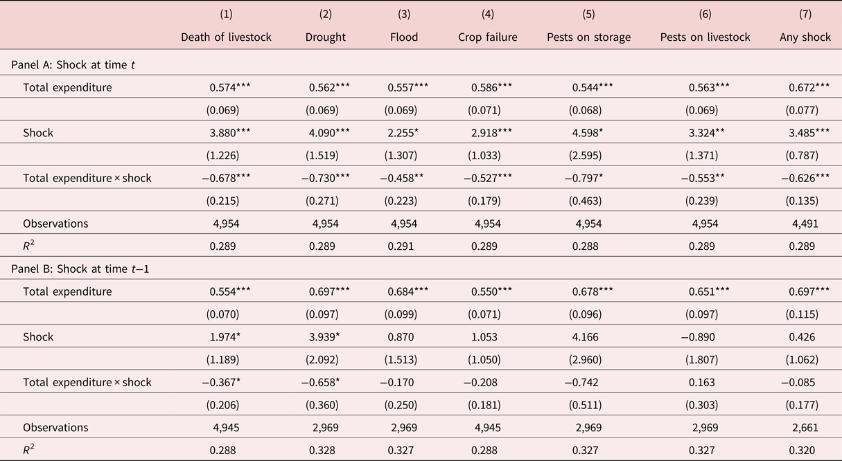
Notes: Estimated using OLS. Robust standard errors in parentheses. Other control variables include child gender and age, mother's age and education, father's age and education, household size, and an indicator for rural areas.
***p < 0.01, **p < 0.05, *p < 0.1.
To examine the social gradient in the response to the shocks, we interact household expenditure with the respective shock variables.Footnote 23 We consistently observe a negative coefficient on the interaction term indicating a decreasing effect of the shocks with increasing household expenditure (Panel A). In other words, the impact of the shocks is larger for children from low expenditure households relative to those from high expenditure households. The shock effects are particularly large and statistically significant for drought and pests on storage. The results in Panel B are largely consistent except that the coefficients of the interaction terms are mostly statistically insignificant, which suggests that the shocks only affect children's health in the short run.
5. Conclusion
This paper provides empirical evidence on the relationship between socioeconomic status and child physical health in Vietnam. In contrast to existing studies, which generally use income or a wealth index to measure socioeconomic status, we use household expenditure (measured using food expenditure and total expenditure) as an alternative measure. The concerns raised in the existing literature over the use of a composite wealth index as well as issues with measuring income within a developing country context endorse our focus on household expenditure. Using expenditure instead of income also allows us to explore the mechanisms via which income affects child health, in which household consumption plays an important role. Moreover, in contrast to the existing literature, which tends to focus on subjective health measures, we exploit a set of objective measures of child health, namely, BMI, standardized BMI (BMI-Z) and standardized height (HAZ). This allows us to examine the effect of expenditure in both the short run (using BMI) and the long run (using height). Finally, the potential endogeneity of household expenditure is addressed using an IV approach, with the local unemployment rate and rainfall deviation used as instruments. We provide a number of robustness checks that lend substantial empirical support toward our identifying assumptions as well as our findings.
Our results indicate a strong statistically significant relationship between household expenditure and child health. We find evidence that expenditure impacts on child health both in the short run, as captured by changes in BMI, and via the accumulative effects of poor nutrition on height, in the long run. Specifically, we find that a 10% increase in total expenditure (food expenditure) is associated with a 0.013 (0.015) increase in BMI. This translates into a weight gain of 213 (541) grams in a “typical” child in our sample. The results are also generally consistent across the various measures of health outcomes, notably BMI-Z and HAZ. For example, a 10% increase in food expenditure is associated with increases of 0.10 and 0.23 of a standard deviation in BMI and height, respectively. We also examine our results across two different age groups, children aged from 4 to 9 years, and children aged from 10 to 16 years. Overall, we find consistent effects of expenditure across both age groups. Finally, we examine the effect of a range of exogenous adverse economic shocks on children's health. We find that the effects of the shocks are greater for children from lower socioeconomic backgrounds.
Our findings highlight the importance of health policy interventions especially for children living in rural areas with low economic development and poor healthcare services. Existing policies in Vietnam, such as public health insurance programs, have focused on health care provision. Nonetheless, many households opt for private health providers in order to get treated quickly [Nguyen (Reference Nguyen2016)]. This results in an increase in health care expenditure (i.e., out-of-pocket expenditure) that may potentially lead poor households into a poverty trap. Our findings demonstrate that policies which directly impact on household resources, such as a food subsidy and/or cash transfer programs, are likely to have a significant effect on children's health and well-being both in the short run and long run. In turn, in the longer term, enhanced child health outcomes can potentially lead to higher educational attainment, improved labor market outcomes, and better health later in life, which may serve to combat intergenerational transmission issues.
Conflict of interest
The authors declare that they have no conflict of interest.


