


Introduction
During growth, anatomical elements of organisms expand and make contact with one other to generate higher-level morphological entities. Packing, orientation, shape, and size of anatomical elements determine connectivity patterns among them. In turn, this connectivity induces morphogenetic changes that constrain the shape and development of each anatomical element (Rasskin-Gutman Reference Rasskin-Gutman2003). Describing patterns of connectivity among organs is essential for identifying anatomical homologies among taxa and assessing morphogenetic processes and their evolution (Rieppel Reference Rieppel1988; Rasskin-Gutman Reference Rasskin-Gutman2003). Following Geoffroy Saint-Hilaire’s “Principe des connexions” (1818), connectivity of body parts is a more important criterion for recognizing homologies among taxa than function and shape (Geoffroy Saint-Hilaire Reference Geoffroy Saint-Hilaire1818; Rasskin-Gutman and Esteve-Altava Reference Rasskin-Gutman and Esteve-Altava2014). This is particularly relevant for studies of organisms with skeletons (or parts of them) made of discrete elements such as arthropods, vertebrates, or echinoderms. Nonetheless, comparatively few studies devoted to morphological analyses have developed comparative frameworks with proper tools to explore the evolution of organization patterns (see, however, Rasskin-Gutman and Buscalioni Reference Rasskin-Gutman and Buscalioni2001; Rasskin-Gutman Reference Rasskin-Gutman2003; Esteve-Altava et al. Reference Esteve‐Altava, Marugán‐Lobón, Botella and Rasskin‐Gutman2011; Esteve-Altava and Rasskin-Gutman Reference Esteve-Altava and Rasskin-Gutman2014; Rasskin-Gutman and Esteve-Altava Reference Rasskin-Gutman and Esteve-Altava2014).
Graphs are convenient ways of representing connectivity patterns between objects from a certain collection. A graph is a set of nodes connected pairwise by a subset of edges that can be oriented, valued, signed, or not (Lesne Reference Lesne2006). It can be associated with abstract relationships within an arbitrary set of points, or with a real space corresponding to topological structures. Graph studies are at the crossroads of many areas of science, from mathematics to architecture (Baglivo and Graver Reference Baglivo and Graver1983), biology (Beck et al. Reference Beck, Benkö, Eble, Flamm, Müller and Stadler2004; Samadi and Barberousse Reference Samadi and Barberousse2006; Lesne Reference Lesne2006), biomedicine (Barabási and Oltvai Reference Barabási and Oltvai2004; Hosseini et al. Reference Hosseini, Hoeft and Kesler2012), and social sciences (Newman et al. Reference Newman, Watts and Strogatz2002). At the crossroads of mathematics and biological sciences, tools and statistics derived from graph theory—which concerns the study of mathematical structures—can be used to analyze graph representation of biological structures and assess their evolutionary patterns (Rasskin‐Gutman Reference Rasskin-Gutman2005; Dera et al. Reference Dera, Eble, Neige and David2008; Esteve‐Altava et al. Reference Esteve‐Altava, Marugán‐Lobón, Botella and Rasskin‐Gutman2011; Rasskin-Gutman and Esteve-Altava Reference Rasskin-Gutman and Esteve-Altava2014).
Recently, Zachos and Sprinkle (Reference Zachos and Sprinkle2011) modeled skeletal growth of echinoids using directed graphs to represent sequences of plate addition. Tools of graph theory have occasionally been applied specifically to studies of topological structures in biological models. Rasskin-Gutman and Buscalioni (Reference Rasskin-Gutman and Buscalioni2001) and Rasskin-Gutman (Reference Rasskin-Gutman2003) have used graphs to study form change and evolution of the vertebrate skeleton. They represented topological relations among skeletal elements as a graph, each bone corresponding to a node and the boundaries formed by adjacent bones as edges that join those nodes. They generated a comparative framework as a morphospace of connections and explored it to assess macro-evolutionary patterns of form change. Esteve-Altava et al. (Reference Esteve‐Altava, Marugán‐Lobón, Botella and Rasskin‐Gutman2013a, Reference Esteve‐Altava, Marugán‐Lobón, Botella and Rasskin‐Gutman2013b) studied the structural constraints associated with the evolution of tetrapod skull complexity, as well as the integration and modularity of the human skull, using graph analysis and statistics derived from graph theory.
As in vertebrates, the echinoderm skeleton consists of many discrete elements (named plates or ossicles) that contact each other as in sea urchins or sea stars. Boundary patterns among these elements determine the shape of higher-level anatomical entities or organs, and are therefore essential to systematics and studies of echinoderm evolution (David et al. Reference David, Lefebvre, Mooi and Parsley2000). Echinoids represent an important component of post-Paleozoic echinoderm diversity (Erwin Reference Erwin1993). They experienced a large post-Paleozoic diversification that led to the emergence of manifold morphologies, well illustrated with the evolution of irregular echinoids (Kier Reference Kier1974; Smith Reference Smith1984). Having originated in the Early Jurassic (Jesionek-Szymańska Reference Jesionek-Szymańska1970; Smith Reference Smith1984; Smith and Anzalone Reference Smith and Anzalone2000; Saucède et al. Reference Saucède, Mooi and David2007) irregular echinoids diversified greatly as early as the Middle Jurassic (Thierry and Néraudeau Reference Thierry and Néraudeau1994), this evolutionary radiation being among the most significant events of echinoid evolution. Irregular echinoids—the atelostomates—include forms as diverse as the present-day lamp urchins, heart urchins, and sand dollars, and constitute nearly 60% of extant and extinct species of echinoids (calculated from Kier Reference Kier1974). Irregular echinoids are distinguished from other regular, globose echinoids (Fig. 1A) largely by their bilateral symmetry, which appears secondarily during growth and alters the pentaradial shape of the test (Fig. 1B). The establishment of the secondary bilateral symmetry is associated with several drastic changes in the way skeletal elements are interconnected. One of the most evolutionary significant concerns the plate pattern of the apical disc, which is highly transformed by the migration of the periproct—the area that contains the echinoid excretory organ—from the top of the test toward its posterior margin at early ontogenetic stages. During this morphogenetic process, the periproct moves out of the apical disc, a skeletal structure comprising ten skeletal elements, the five genital and five ocular plates (Fig. 1), and involved in essential biological functions such as reproduction, inner pressure control, and growth (new coronal plates form in close contact with ocular plates during growth). Although the first irregular echinoids retained the apical plate pattern of regular echinoids, that is, with the periproct still enclosed within the apical disc (Jesionek-Szymańska Reference Jesionek-Szymańska1970; Smith and Anzalone Reference Smith and Anzalone2000), one key morphological innovation associated with their subsequent diversification was the achievement of the so-called exocyclic pattern (Fig. 2A), in which the periproct and apical plates—genitals and oculars—are completely disjunct (Kier Reference Kier1974; Smith Reference Smith1984). The evolutionary trend of the periproct to move away from the apical disc has been achieved independently in the different subgroups of irregulars throughout the Jurassic (Jesionek-Szymańska Reference Jesionek-Szymańska1963; Mintz Reference Mintz1966; Saucède et al. Reference Saucède, Mooi and David2007). This migration accompanied other morphological innovations such as the anteriorly placed mouth, the single-direction locomotory systems with spines specialized to produce an efficient forward power-stroke, and the miniaturization of almost all external appendages such as spines and podia. All these morphological innovations are deeply linked with the colonization of and adaptation to new habitats, determined by the nature of the sea bottom (soft sediments) where irregular echinoids live (Smith Reference Smith1984; Barras Reference Barras2008).

Figure 1 Structure of the apical disc of echinoids. A, In regular echinoids, the periproct is enclosed within the apical disc, a composite structure that comprises five ocular and five genital plates surrounding the periproct. B, In Atelostomata and other irregular echinoids, the migration of the periproct leads to a breaking of the apical disc region into the genital and ocular plates, which stay in an apical position, and the periproct, which moves toward the margin of the test (modified after Saucède et al. Reference Saucède, Mooi and David2007).

Figure 2 Echinoid apical plating and associate graphical representations. A, Two highly contrasting apical systems observed in regular echinoids (left) and Spatangoida (right). Left: Example of the regular echinoid Diplocidaris gigantea (L Agassiz) – (after Kier Reference Kier1974: Fig. 42A). Genital plates (dark gray) are labeled G1 to G5 and are perforated by gonopores (black circles) - G2 is also perforated by hydropores; ocular plates (in white) are labeled OI to OV and are perforated by tiny ocular pores. In regular echinoids, there are ten apical plates (five genitals and five oculars) organized into two concentric rings surrounding the periproctal area (white area in the center of the apical disc). Right: Example of the spatangoid Asterostoma excentricum Agassiz (after Fischer Reference Fischer1966: Fig. 502–1D). In Spatangoida, there are nine apical plates (four genitals and five oculars) with no periproctal area in the center. B, Connectivity graph: All potential pairwise contacts between plates can be represented as a graph in which edges represent the potential contacts and nodes represent the plates (genital plates as dark squares and ocular plates as white circles). There are 45 possible contacts between ten plates in regular echinoids (left) vs. 36 between nine plates in Spatangoida (right). One single graph represents all possible plate contacts for all apical systems with an equal number of plates. C, Contact graph: Real contacts observed between apical plates of a specimen can be represented as edges in a contact graph, one single graph corresponding to one unique connectivity pattern.
As with most other irregular echinoids, atelostomates originated during the Early Jurassic and first diversified in the Middle Jurassic. They have been the most diversified group of echinoids ever since. They number approximately 1600 fossil and Recent species, representing about 25% of post-Paleozoic species of echinoids (Kier Reference Kier1974) and showing high levels of morphological disparity early in their history (Eble Reference Eble2000). In atelostomates, there are between six and ten apical plates—located at, or close to, the top of the test—that constitute the apical disc. The boundary patterns among apical plates have always been a concern of systematists. The way these patterns have evolved over long periods of time is key to understanding echinoid macroevolution (Kier Reference Kier1974; Saucède et al. Reference Saucède, Mooi and David2004, Reference Saucède, Mooi and David2007), so they have been widely used to determine the classification and phylogeny of Atelostomata (Fisher Reference Fischer1966; Wagner and Durham Reference Wagner and Durham1966; Kier Reference Kier1974; Smith Reference Smith1984; Kroh and Smith Reference Kroh and Smith2010).
Analyzing and quantifying the diversity of connectivity patterns among plates across major clades and over a macro-evolutionary time scale is challenging. At such taxonomic and temporal scales, morphological diversity is represented by very contrasting connectivity patterns including phenomena of plate loss, position shift, and disjunctions into separate modules (Fig. 3). Here, the main question we address regards the evolution of apical plate diversity that led to the emergence and diversity of atelostomate echinoids. How did topological patterns of plate connectivity evolve over time? Which morphogenetic constraints drove their evolution? How are plate numbers and connectivity patterns among those plates associated in atelostomate echinoids? Are plate loss and restructuration of apical systems associated with simplification, or with complexification as in the evolution of the tetrapod skull (Esteve-Altava et al. Reference Esteve‐Altava, Marugán‐Lobón, Botella and Rasskin‐Gutman2013a)? How diversified are the connectivity patterns observed in nature compared to what theory predicts? To address all these questions, we analyzed graph representation of plate structures, using tools and statistics of graph theory. To assess how forms predicted by graph theory encompass and exceed those observed in nature, we generated a comparative framework as a morphospace of connections, in which the diversity of plate patterns observed in nature was mapped and analyzed.

Figure 3 Studied groups of atelostomate and basal irregular echinoids along with main phylogenetic relationships. These apical systems with their associated contact graphs illustrate the diversity of connectivity patterns (modified after Saucède et al. Reference Saucède, Mooi and David2007). A, Diplocidaris gigantea (Agassiz Reference Agassiz1840) (modified after Kier Reference Kier1974: Fig. 42A); B, Plesiechinus hawkinsi Jesionek-Szymańska Reference Jesionek-Szymańska1970 (after Saucède et al. Reference Saucède, Mooi and David2007: Fig. 2E); C, Pygaster gresslyi Desor Reference Desor1842 (after Saucède et al. Reference Saucède, Mooi and David2007: Figs. 2F, 4B); D, Orbigniana ebrayi (Cotteau 1869) (after Saucède et al. Reference Saucède, Mooi and David2007: Fig. 3E); E, Pygorhytis ringens (Agassiz Reference Agassiz1839) (after Saucède et al. Reference Saucède, Mooi and David2007: Figs. 3D, 4F); F, Stereopneustes relictus de Meijere Reference Meijere de1902 (after Saucède et al. Reference Saucède, Mooi and David2004: Fig. 3); G, Pourtalesia miranda Agassiz Reference Agassiz1869 (after Saucède et al. Reference Saucède, Mooi and David2004: Fig. 3); H, Toxaster granosus var. kiliani Lambert Reference Lambert1902 (modified after Devriès Reference Devriès1960: Fig. 12); I, Toxaster subcavatus (Gauthier 1875 in Cotteau, Péron and Gauthier 1873–Reference Cotteau, Péron and Gauthier1891) (modified after Masrour Reference Masrour1987: Fig. 49B); J, Echinocardium cordatum Pennant Reference Pennant1777 (modified after David Reference David1985a: Fig. 9E). In black: periproct, gonopores, and hydropores; dark gray: supplementary plates; light gray: genital plates; white: ocular plates.
Materials and Methods
Data Collection
We conducted an extensive survey of drawings and figures published over half a century (e.g., Mortensen Reference Mortensen1950, Reference Mortensen1951; Fischer Reference Fischer1966; Wagner and Durham Reference Wagner and Durham1966; Kier Reference Kier1974) along with material and reference specimens from academic collections to make as complete as possible the inventory of the apical plating diversity evolved in Atelostomata from the origin of the clade to the present day (Supplementary Table 1). Data on apical plate patterns were stored in the inventory as pairwise connectivity patterns between genital and ocular plates regardless of the taxonomic ranking of apical variations, either within species or between genera or families. Reference species and specimens were listed (Supplementary Table 1) for each recorded boundary pattern; this does not preclude the possibility of similar patterns occurring in other taxa. The taxonomic value of boundary patterns was all limited to three groupings within the Atelostomata: the paraphyletic basal atelostomates, and the two clades Holasteroida and Spatangoida, across seven time periods: Early Jurassic, Middle Jurassic, Late Jurassic, Early Cretaceous, Late Cretaceous, Paleogene and Neogene, and Present. For comparison and discussion, apical plate patterns were also documented for basal Irregularia along with one reference pattern chosen as representative of the ancestral pattern occurring in regular echinoids (Fig. 3). All the pairwise boundary patterns we considered were between the ten apical plates (genital and ocular plates) for which homologies among all echinoids are well established (Saucède et al. Reference Saucède, Mooi and David2004, Reference Saucède, Mooi and David2007); supplementary plates (e.g., catenal) occurring in basal Irregularia and basal atelostomates were not taken into account because, being highly variable in number and arrangement, homologies within this category of plates are not yet clearly understood (Saucède et al. Reference Saucède, Mooi and David2004, Reference Saucède, Mooi and David2007).
Graph Representation
To describe and explore the diversity of connectivity patterns between plates, each pattern was symbolized as a graph in which plates are coded as nodes that are pairwise connected by edges. In Figure 2, two contrasting apical patterns are shown along with their respective graphical representations. In regular echinoids (left), the plesiomorphic apical disc comprises ten apical plates (five genitals and five oculars) organized into two concentric rings surrounding the periproctal area (Fig. 2A). In Spatangoida (right), there are up to nine apical plates (four genitals and five oculars) with no central periproctal area. All potential pairwise contacts between plates were represented as a fully connected graph, herein referred to as a connectivity graph (Fig. 2B). There are 45 possible contacts between ten plates in regulars (left) vs. 36 between nine plates in Spatangoida (right), though all contacts cannot exist at the same time in nature. Conversely, real contacts between plates that do occur in nature in a given apical pattern can be represented as edges of a realized graph, one single graph corresponding to one unique connectivity pattern (Fig. 2C).
In graph theory, a possible way to summarize information of a graph is to build an adjacency matrix (noted M here). For a graph containing n nodes, this matrix corresponds to a n by n square matrix, where entries M ij are set to 1 if an edge occurs between nodes i and j, or to 0 otherwise. M is symmetric, and only its triangular upper (or lower) part, without the diagonal, is informative. This triangular upper part can be stored in a (n 2−n)/2 vector, so that when studying a set of k graphs, all the adjacency information of this data set can be stored in a k by (n 2−n)/2 matrix, here named matrix MA. In this study, all collected data were compiled in MA with n ranging from six to ten apical plates for k=145 echinoid patterns (Table 1). For specimens with fewer than ten apical plates, the absence of a plate implies that theoretical contacts to this plate are coded 0. This implies that some connectivity patterns are duplicated in Table 1 when corresponding apical discs differ in plate number.
Table 1 PCA's eigenvalues and eigenvectors for the four topological indices.

Graph Simulations
To appraise the extent to which real patterns of apical plate contacts are diversified, we needed elements of comparison. Graph simulations were run in order to generate such a comparative framework. Two sets of 100,000 random graphs were generated: the first one leaving the equal probability (50%) for an edge to be present or absent, and the second set attributing edge probabilities according to real contact frequencies as recorded in matrix MA. Other probability values were tested but only the two most contrasting ones are presented here for demonstration purposes. A fundamental condition for observed and simulated graphs to be compared is that all simulated graphs must be planar. Real echinoid tests are curved; planar surfaces and contacts between apical plates occur only in this curved plane, which is a two-dimensional space. An immediate consequence of planarity is that an n-node planar graph cannot admit more than 3n-6 edges. To test simulated graphs for planarity, we used the Boyer-Myrvold algorithm (Boyer and Myrvold Reference Boyer and Myrvold2004) implemented in Matlab® (bgl toolbox). After the test, 100,000 planar graphs were retained for each set. They all include a number of connected nodes ranging from four to ten, that is, the range of plate numbers observed in matrix MA. All codes used for analyzing our data are available upon request from the first author.
Edge Frequencies
The effect of sampling bias on the distribution of real plate contact frequencies was quantified as a 95% confidence interval for each frequency value. From matrix MA, 10,000 bootstrap samples were generated by randomly picking with replacement 145 graphs for each sample. Additionally, Fisher’s exact tests were performed to check whether the two sets of simulated graphs reflected the distribution of contact frequencies observed in matrix MA.
Topological Indices
To quantify apical topologies, four indices were used. They all take into account the number of nodes, the number of edges, and the radius of graphs (see details below). Based on the adjacency matrix, here the number of nodes only refers to the number of connected nodes; potential isolated nodes were not considered. For both realized and simulated graphs, connected and disconnected graphs were distinguished. Connected graphs are graphs for which connected nodes constitute a unique graph, whereas disconnected graphs are those composed of at least two isolated components, or sub-graphs. Respective procedures for computation of topological indices of connected and disconnected graphs are different. Details of the two procedures are given below and only refer to graphs with four to ten connected nodes (e.g., the range observed in the data set, matrix MA).
Density Index
The density index (D) quantifies the density of edges occurring in a graph. Graph theory predicts that the maximal number of edges is 3n-6 (with n>2) in planar graphs. Thus, the density index is defined as the ratio of the realized number of edges (noted e) over the theoretical maximal number of edges:
 $$D={e \over {3n{\minus}6}}$$
Practically, in the echinoid apical disc, the density index quantifies the relative number of contacts really existing among plates compared to the theoretical maximum. It gives an idea of how compact or, conversely, loose apical discs are.
For connected graphs, we have
 $${{n{\minus}1} \over {3n{\minus}6}}\leq D\leq 1$$
For disconnected graphs, if at least one connected component has more than 2 nodes, we have
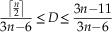 $${{\left\lceil {{n \over 2}} \right\rceil } \over {3n{\minus}6}}\leq D\leq {{3n{\minus}11} \over {3n{\minus}6}}$$
where  $$\left\lceil {{n \over 2}} \right\rceil $$
denotes the ceiling function.
$$\left\lceil {{n \over 2}} \right\rceil $$
denotes the ceiling function.
D equals 1 when all possible edges are present. In disconnected graphs, e and n are respectively the number of edges and number of connected nodes in all sub-graphs, so that on average D is expected to have lower values for disconnected graphs than for connected graphs.
Eccentricity Index
The radius R of a graph is the minimal eccentricity of its nodes, the eccentricity of a node being the longest distance (measured in number of edges) separating this node from any other node. For disconnected graphs, we set R to be the averaged radius of connected components weighted by the number of corresponding nodes:
 $$R={1 \over n}\mathop \sum\limits_{i=1}^K n_{i} R_{i} $$
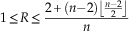
where n i and R i are, respectively, the number of connected nodes and the radius for the i th sub-graph among K. In the apical disc, the eccentricity index quantified how elongated apical discs are. For connected graphs, R ranges between 1 for star-like graphs (e.g., all edges connect to a central node) and n/2 or (n-1)/2, depending on the parity of n, for chain-like graphs. Hence, we have
 $$1\leq R\leq \left\lfloor {{n \over 2}} \right\rfloor $$
where  $\left\lfloor {{n \over 2}} \right\rfloor $
denotes the floor function; and for disconnected graphs,
$\left\lfloor {{n \over 2}} \right\rfloor $
denotes the floor function; and for disconnected graphs,
 $$1\leq R\leq {{2{\plus}(n{\minus}2)\left\lfloor {{{n{\minus}2} \over 2}} \right\rfloor } \over n}$$
Complexity Index
From the radius, we defined an index of complexity (noted C), which is the ratio of the number of edges in a graph over twice the radius of the graph (or twice the weighted mean radius for disconnected graphs):
 $$C={e \over {2R}}$$
Practically, the complexity index refers to the number of connections existing among plates, taking into account the stretching of the apical disc: the more clustered the contacts among plates are, the more complex the apical disc is.
C will be minimal when e is minimal and R maximal (e.g., chain-type graphs), and maximal in the opposite case (e.g., star-like graphs with all possible edges). For connected graphs, we have
 $${{n{\minus}1} \over {2\left\lfloor {{n \over 2}} \right\rfloor }}\leq C\leq {{3n{\minus}6} \over 2}$$
and for disconnected graphs,
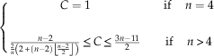 $$\eqalignno{ & \left\{ {\matrix{ {C=1} & {} & {{\rm if }\quad \,n=4} \cr {} & {} & {} \cr {{{n{\minus}2} \over {{2 \over n}\left( {2{\plus}\left( {n{\minus}2} \right)\left\lfloor {{{n{\minus}2} \over 2}} \right\rfloor } \right)}}\leq C\leq {{3n{\minus}11} \over 2}} & {} & {{\rm if}\quad \,n\,\gt\, 4} \cr } } \right. \cr & $$
Asymmetry Index
To quantify the asymmetry level of a graph (noted A), e.g., how unevenly connected the nodes of a graph are, we computed the variance of node degree (noted d). In graph theory, the degree of a node is the number of edges connected to the node. This asymmetry index is
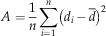 $$A={1 \over n}\mathop \sum\limits_{i=1}^n \left( {d_{i} \,{\minus}\,\bar{d}} \right)^{2} $$
Hence, the asymmetry index quantifies whether contacts among plates are evenly distributed over the apical disc or not.
For disconnected graphs, A will be the averaged asymmetry of connected components weighted by the number of corresponding nodes:
 $$A={1 \over n}\mathop \sum\limits_{i=1}^g n_{i} A_{i} $$
where A i is asymmetry for the i th sub-graph.
Connected graphs have a minimal asymmetry of 0, when all nodes have the same number of edges. The maximal value of A was determined in a previous study (Caro and Yuster Reference Caro and Yuster2000), and characterizes graphs where few nodes concentrate all contacts. The asymmetry range is:
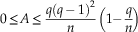 $$0\leq A\leq {{q(q\,{\minus}\,1)^{2} } \over n}\left( {1{\minus}{q \over n}} \right)$$
where
 $$q=\left\lfloor {{{3n{\plus}2} \over 4}} \right\rfloor $$
Asymmetry of disconnected graphs is minimal when the nodes of all connected components have the same degree. The upper bound is reached for two connected components, one having two nodes:
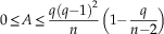 $$0\leq A\leq {{q(q{\minus}1)^{2} } \over n}\left( {1{\minus}{q \over {n{\minus}2}}} \right)$$
where
 $$q=\left\lfloor {{{3n} \over 4}{\minus}1} \right\rfloor $$
Topological Space
Index values were explored using principal component analyses (PCAs) computed on index correlation matrices. PCAs allow building empirical spaces defined by uncorrelated axes in which morphological disparity can be conveniently described (Foote Reference Foote1993; Wills et al. Reference Wills, Briggs and Fortey1994; Roy and Foote Reference Roy and Foote1997; Erwin Reference Erwin2007). The empirical space corresponds to a morphospace of connections between plates (or boundary patterns) here named topological space. Such a topological space can be conveniently used to describe the disparity of apical topologies as quantified using the four topological indices: the density, eccentricity, complexity, and asymmetry of graphs. PCAs were performed on these indices. Simulated graphs were used to get a minimal estimate of the sub-space of possible planar graphs, one PCA for each set of simulated graphs. In order to describe the evolution of topological disparity across the different time periods and echinoid groups, PC scores were partitioned into seven time plots, one for each time period, as well as into four group plots, one for each echinoid group. Topological disparity was quantified for each time period and group, using the method described by Dommergues et al. (Reference Dommergues, Laurin and Meister1996). First, the space defined by the four PCA axes was subdivided into a regular grid of 4-D hypercubes. Then, disparity of each plot (time and group plots) was estimated as the number of hypercubes covered with observed values standardized by the number of hypercubes covered with values of simulated graphs. This standardized value is named Percentage of Morphospace Occupation (PMO; Dommergues et al. Reference Dommergues, Laurin and Meister1996). In contrast to traditional disparity metrics, it does not assume that the studied space is Euclidean. However, like other range-based disparity metrics, PMO values are sensitive to sample size. Consequently, we performed a rarefaction procedure to correct PMO values for the effect of sample size (see, e.g., Navarro Reference Navarro2003), and a bootstrap procedure to test for potential sampling bias. One thousand bootstrap samples were generated and rarefied to the lowest number of graphs counted in a period and in a group, for time periods and taxonomic groups respectively. Then, for each time and group plot, the number of hypercubes was divided by the number of hypercubes covered with simulated graphs. Finally, bootstrap means and 95% confidence intervals were computed. Analyses were realized using the software Matlab®.
Results
Connectivity Patterns
According to graph theory, 210*9/2≈3.52×1013 different (not necessarily connected) labeled graphs can be constructed with ten elements and 29*8/2≈6.87×1010 with nine elements (total number of non-isomorphic graphs); this is the maximum number of possible connectivity patterns. However, because apical plates connect to each other in a two-dimensional space—the echinoid test surface—we considered only planar graphs. The total number of possible labeled, graphs is ≈32×1010 for planar graphs with ten nodes and ≈2×10¹⁰ for planar graphs with nine nodes. Because there are from six to ten apical plates in atelostomates, the total number of possible planar graphs with six to ten nodes is ≈3.42×10¹¹ (Bodirsky et al. Reference Bodirsky, Groepl and Kang2003). From our extensive survey of literature, along with our own observations, we were able to identify 116 different boundary patterns only in adult atelostomates, that is, 116 different ways apical plates connect to each other. In addition, 18 other patterns were identified in basal irregulars and one additional pattern was considered to represent the ancestral regular pattern. This relatively low topological disparity with regard to predictions of graph theory suggests the existence of strong morphogenetic constraints.
According to graph theory, the maximum number of edges in a graph with n nodes is n(n−1)/2. This number declines to 3n−6 in a planar graph. Figure 4 depicts the relation between the maximum number of edges across the number of nodes for non-planar graphs, for planar graphs, and the real number of edges observed in echinoids. Overall, contact numbers in echinoids never reach the maximum theoretical number computed for planar graphs. They do not show extremely low values either but vary into the range of average theoretical values computed for planar graphs. A more detailed examination shows that within echinoids, variation in the number of contacts differs among groups. Contact numbers are highly variable in basal irregulars, basal atelostomates, and holasteroids, but they are confined to high values in spatangoids.

Figure 4 Distribution of the observed number of contacts vs. the number of plates. Dark gray area for impossible graphs; shaded gray area for non-planar graphs, which are impossible graphs for 2-D structures.
In addition to the total number of boundary patterns and overall number of contacts per pattern, we analyzed the observed frequency of each contact in echinoid patterns to investigate those patterns in more detail; specifically, we computed the frequency of contacts for each pair of plates and each plate independently (Fig. 5). The ranked frequency distribution of the 45 possible contacts between pairs of plates (e.g., frequency of each of the 45 labeled edges potentially connecting the ten nodes of graphs) is plotted Figure 5A. The distribution is lognormal, showing that the observed frequency of contacts is extremely heterogeneous among plates. The bootstrap procedure supports the robustness of data (narrow 95% CI) and the Fisher’s exact test performed between the observed distribution and the distribution based on the first set of simulated graphs (50/50 edge probability) is significant (p<0.001). This confirms that contact frequencies differ significantly among plate pairs. In contrast, the Fisher’s exact test performed between the observed distribution and the distribution of the second set of simulated graphs is not significant (p=1). It shows that the second set of simulated graphs matches the observed contact frequencies. Figure 5B shows the ranked values of contact numbers for each plate separately; 71% of contacts occur between ocular-genital mixed plate pairs (1090 recorded contacts over 1538 in all). This can easily be explained by the alternate pattern of ocular and genital arrangement in apical systems, most contacts occurring between adjacent plates. Numbers of contacts with genital plates are homogenously distributed, except for genital 5, which is absent in most atelostomates, and genital 2, which is contacted is a little more frequently than other genitals. Contacts with anterior ocular plates OIV and OII are more frequent than with other oculars.

Figure 5 Observed contact frequency between apical plates. A, Ranked frequency distribution of contacts between the 45 possible pairs of apical plates (the 95 % confidence interval was computed by bootstrapping). B, Ranked frequency values plotted for contacts between all genitals and oculars (O-G), all genitals (G-G), and all oculars (O-O) taken together, and for each apical plate separately (G2 to OV).
The observed frequencies of contacts between plate pairs were also plotted in rose diagrams and data were synthesized for each of the five following groups separately: regulars, basal Irregularia, basal Atelostomata, Holasteroida, and Spatangoida (Fig. 6A–E). A rose diagram is a circular histogram that mimics the apical structure to help visualize topological data in space. In a rose diagram, each apical plate is associated with one sector into which all possible contacts with other plates (nine in regular echinoids vs. eight in Spatangoida and Holasteroida) can be represented as a bar, with the longest bar having the highest frequency. In Figure 6A the frequency of contacts forms a star-shaped symmetrical plot: contacts exclusively occur between adjacent plates of the apical ring, namely between oculars and genitals. There are some transverse contacts as well, all of which occur between genital pairs. The frequency pattern in basal Irregularia (Fig. 6B) differs from the previous one mostly in contact loss between posterior plates and genital 5. This is the case of disconnected apical systems. Frequency also differs in the occurrence of transverse contacts between oculars OII and OIV and the absence of these contacts between genital pairs. In basal Atelostomata (Fig. 6C), the antero-posterior asymmetry is the most obvious feature, as exemplified by common disjoined plates of the posterior part of apical systems. First, contact loss between genital 5 and other apical plates is almost the rule, and transverse contacts (OV-OI and G1-G4), when present, predominate over contacts between adjacent plates (OV-G4 and OI-G1). Anteriorly, plate contacts with genital 2 dominate over contacts with genital 3. In Holasteroida (Fig. 6D), besides the absence of genital 5 in the apical disc, the main features are the prevalence of transverse contacts (G4-G1, IV-OII, OIV-G2), exemplified by the so-called intercalary plate patterns, and the loss of contacts with genital 3 in favor of contacts with genital 2. In Spatangoida (Fig. 6E), in addition to the absence of genital 5 in the apical disc, the main feature is the prevalence of contacts with genital 2, which constitutes a hub-like plate in the anterior part of apical systems. Posteriorly, contacts with genital 4 dominate over those with genital 1. This prevalence of transverse contacts with genitals 2 and 4 has long been described in the literature as “compact” apical plating. This corresponds to a transverse asymmetry of contact distribution in apical systems, contacts that are concentrated in the anterior-right and posterior-left parts of apical systems.

Figure 6 Rose diagrams showing contact frequency between pairs of apical plates in five echinoid groups: the regular echinoids (A), basal Irregularia (B), basal Atelostomata (C), Holasteroida (D), and Spatangoida (E). Bold and circled plate numbers highlight the plates that are the most frequently contacted.
Plate Topologies
This section aims to characterize and quantify topological features of entire apical plate arrangements. In atelostomates, the disparity of plate patterns implies the need to use several metrics to quantify different topological features. Four indices were computed to quantify the density, eccentricity, complexity, and asymmetry of apical patterns—four features that are expected to show a wide range of variation according to literature (Jesionek-Szymańska Reference Jesionek-Szymańska1970; Kier Reference Kier1974; Smith Reference Smith1984; Saucède et al. Reference Saucède, Mooi and David2007). The theoretical range of all possible density values is relatively constant for connected patterns, whatever the plate number (Fig. 7A,B; solid lines), while it increases with plate number for disconnected patterns (Fig. 7A,B; dashed lines). In contrast, maximum theoretical values and their range increase with plate number for the eccentricity, complexity, and asymmetry of both connected (solid lines) and disconnected (dashed lines) patterns (Fig. 7). Overall, plate patterns show low-density values compared to theoretical maxima, some values even matching theoretical minima. Overall, this means that most plate patterns are loose structures in atelostomates; that is, fewer apical plates are connected to each other than graph theory would predict. In contrast, eccentricity values in connected patterns are highly variable (black crosses), some matching either theoretical minima or maxima, whereas disconnected patterns (open circles) show minimum to mean values depending on plate number. In other words, eccentricity of connected apical systems is highly variable, whereas disconnected patterns are composed of comparatively more compact entities. Accordingly, the complexity of disconnected patterns is relatively high, whereas connected patterns have low complexity values, some matching the theoretical minimum, except for some patterns composed of eight and nine plates. The asymmetry of contact distribution within apical systems is highly variable in systems with fewer than eight plates. Eight-plated to ten-plated systems show decreasing asymmetry values with increasing plate number, meaning that contacts tend to be more evenly distributed among plates when plate number increases.

Figure 7 Density, eccentricity, asymmetry, and complexity values versus plate number for observed (black crosses and open circles) and simulated (orange hatched and green shaded areas) data. Left, The four topological indices with simulated data based on a 50/50 percent probability of edge occurrence/absence. Right, The four topological indices with the second set of simulated data. Solid gray lines show theoretical maximum and minimum index values for connected graphs. Dashed gray lines show theoretical maximum and minimum index values for disconnected graphs. Black crosses: observed connected graphs; open circles: observed disconnected graphs; orange hatched area: simulated connected graphs; green shaded area: simulated disconnected graphs; the two areas partially overlap.
For all indices, most observed data fall out of the range of values computed from the first set of simulated graphs (based on a 50/50 contact probability between plates) (Fig. 7 left; hatched areas). In contrast, they all fall into the range of values computed from the second set of simulated graphs (Fig. 7 right; hatched areas and unhatched shaded areas). Although this second set of simulated values seems to match observed data, simulated and real data were compared statistically using Chi-square tests performed with R (R Development Core Team 2011). We tested the four indices independently and computed probability values after bootstrap resampling because data were not distributed normally. For all indices, results gave highly significant differences (p<0.01) between the two respective distributions. This means that if plate patterns of atelostomates can be regarded as unlikely according to the first model based on a 50% contact probability, they cannot be accurately simulated by the second model either, in which contact probabilities are based on observed contact frequencies. The mismatch between the first set of simulations and real data indicates that the occurrence of individual contacts between plate pairs is not random and is clearly under the control of structural constraints. The only apparent match between the second set of simulations and real data shows that even if contact probabilities are determined, real patterns cannot be accurately simulated. This implies that entire plate topologies also are under the control of shaping factors and that contacts between plate pairs are covarying units, or modules integrated into a higher-level organization controlling apical topologies.
Morphospace of connections and Disparity Analysis
To fully assess the diversity of apical plate topologies, we used index values of observed data and the two sets of simulations (Table 1) for the first of two PCAs. Not surprisingly, PC score values differ between the two sets of simulations, although respective score ranges are about the same. In addition, observed data fall out of the range of the first set of simulations. A second PCA used index values of observed data and the second set of simulated graphs only (Fig. 8); 82.9% of the total variation is concentrated on the two first PCs (Table 1), so most of the topological disparity can be conveniently described when the two first PCs are plotted together. Eigenvectors were represented in the diagram as segments (red segments in Fig. 8), the length and direction of segments reflecting index contributions to each PC.

Figure 8 Index values of observed (realized) data and a second set of simulated data projected into a topological space (morphospace of connections) that corresponds to the two first axes of the PCA performed on the index correlation matrix. Black crosses: realized connected patterns; open circles: realized disconnected patterns; light gray dots: simulated connected graphs; dark gray dots: simulated disconnected graphs. Blue range bars show the dispersion of score values for simulated connected (Sc) and disconnected (Sd) graphs. Black range bars show the dispersion of score values for observed connected (Oc) and disconnected (Od) patterns. Eigenvectors were represented in the diagram as segments (red segments in upper left corner).
In the general scatter plot (Fig. 8), simulated score values are distributed into distinct clusters that differ in eccentricity mean values, the elongation of clusters reflecting density and asymmetry variations. The uneven distribution of simulated values can be explained by the discrete nature of topological indices from which the PCA was performed. Compared to connected graphs, disconnected graphs are shifted toward negative values on PC2. Such a shift between connected and disconnected graphs, either simulated or real, is due to computation modalities that result in overall lower index values for disconnected graphs. The comparison between blue (simulations – Sd and Sc) and black (observed data – Od and Oc) range bars shows the similarity between the distributions of simulated data and real ones: Distribution ranges are similar but real data seem more evenly scattered. Distributions of real and simulated data were compared for connected and disconnected graphs independently, using a Chi-square test. As for index values (see previous section), distributions of real and simulated data are significantly different, for both connected and disconnected graphs, although real values always fall into the distribution range of simulated data.
Variations of topological disparity were analyzed over time and across taxa by plotting score values for the seven time periods (Fig. 9) and four taxa (Fig. 10) independently. For the Early Jurassic (Fig. 9), one value only is plotted in the extreme top right of the diagram as an outlier relative to simulated data. It corresponds to the apical pattern of the very first irregular echinoid, ‘Plesiechinus’ hawkinsi, which presents a highly eccentric, symmetrical, and loose apical pattern. In contrast, topological disparity clearly increases in the Middle Jurassic as numerous patterns fill in the topological space. Connected patterns (black crosses) are scattered along PC1 (Fig. 9) showing variation in the complexity of patterns, which are mostly represented by basal Irregularia (Fig. 10). Disconnected patterns (open circles) are numerous and plotted in the center of the simulated area. They are mainly represented by basal Atelostomata (Fig. 10). In the Late Jurassic, the disparity of apical patterns covers approximately the same space as in the Middle Jurassic, but connected and disconnected patterns are less numerous. In the Early Cretaceous, the disparity covers a different portion of the topological space. New connected patterns are diversified with asymmetric, dense, and complex structures (Fig. 9). The disparity of these patterns reflects the origination and diversification of Spatangoida (Fig. 10). The Holasteroida are present too, but disparity of patterns is very low. There are a few disconnected patterns (Fig. 9), represented by the very last representatives of basal Atelostomata (Fig. 10). They are characterized by asymmetric, loose, and not very eccentric patterns. Diversity patterns seem to remain unchanged through the Late Cretaceous, Paleogene, and Neogene (Fig. 9), the diversity of apical patterns being represented mainly by the Spatangoida. However, there are some small differences between the three time periods. First, connected patterns in the Paleogene and Neogene are less diversified than in the Cretaceous. They are almost restricted to the center of the diagram, with asymmetric, complex structures that are not very dense, and. In addition, disconnected patterns are almost absent in the Late Cretaceous, Paleogene, and Neogene. They are represented only by a few species within the Holasteroida (Fig. 10). The disparity of present-day patterns strongly contrasts with the three previous time periods (Fig. 9). Most of the topological space is covered, and disparity seems to exceed even the level reached in the Middle Jurassic. Present-day disparity is represented by numerous and diverse patterns, both connected and disconnected. Connected patterns correspond to dense, complex, and asymmetric structures represented by both “modern” Spatangoida and Holasteroida (Fig. 10), whereas disconnected patterns are those of the Holasteroida only, which can have very loose and relatively simple structures (Fig. 10).

Figure 9 Evolution of plate pattern disparity vs. time. Index values of observed and second set of simulated data were projected into a topological space (morphospace of connections) for seven time slices (Early Jurassic to Present). Topological spaces correspond to the two first axes of the PCA performed on the index correlation matrix. Black crosses: realized connected patterns; open circles: realized disconnected patterns; light gray dots: simulated connected graphs; dark gray dots: simulated disconnected graphs. Range bars show the dispersion of score values as in Figure 8.

Figure 10 Disparity of plate boundary patterns across the four studied echinoid taxa. Topological spaces correspond to the two first axes of the PCA performed on the index correlation matrix. Black crosses: realized connected patterns; open circles: realized disconnected patterns; light gray dots: simulated connected graphs; dark gray dots: simulated disconnected graphs. Range bars show the dispersion of score values as in Figure 8.
Results of the PCA clearly indicate that topological disparity varies over time, between the Atelostomata and other Irregularia, and within the Atelostomata themselves (Figs. 9, 10). It varies in terms of realized plate patterns and in terms of overall disparity levels as well. To quantify and compare these apparent variations in disparity levels, we quantified disparity was quantified for each time period and group, using the methodology described by Dommergues et al. (Reference Dommergues, Laurin and Meister1996). Each of the four PCs was subdivided into intervals of one eigenvector unit wide (16 intervals on PC1, 9 on PC2, 9 on PC3, and 7 on PC4), and the 4-D topological space was subdivided into 9072 4-D hypercubes to estimate disparity values using the PMO procedure. The portion of topological space covered with simulated data, that is, the portion of space potentially covered with natural patterns, was subdivided into 406 hypercubes. Of these 406 hypercubes, the realized echinoid disparity varies over time between 2 (5‰) (Early Jurassic) and 44 (108‰) (Present Day), with an apparent increase in the Middle Jurassic and a plateau that extends from the Late Jurassic to the Paleogene and Neogene. Disparity varies across taxa between 14 (34.5‰) (basal Irregularia) and 40 (98.5‰) (Holasteroida), a high disparity value clearly distinguishing this last taxon from other groups (Fig. 11A). However, the uneven number of data present for each time period and taxon (Supplementary Table 1) makes comparisons quite unreliable. For robust comparisons of disparity values across time periods and taxa, data were standardized by rarefaction (Fig. 11B). Overall, real disparity levels are low compared to the topological space covered with simulated graphs (406 hypercubes). However, standardized values of disparity vary significantly over time and across taxa. Hence, mean present-day disparity is significantly higher than during other time periods, the Middle Jurassic excepted, and Holasteroida show a significant higher mean disparity than basal Atelostomata and basal Irregularia.

Figure 11 Raw (A) and rarefied (B) disparity values for the seven time periods and four taxa. Calculation of disparity values is based on the topological space defined by the four PCs of the PCA performed on the index correlation matrix. The portion of topological space covered with simulated data was subdivided into 406 hypercubes, each hypercube being one PC score wide. Disparity values are given as the ratio (‰) of the number of hypercubes covered with observed data over the total number of hypercubes. Rarefied mean values and confidence intervals were computed by bootstrapping (1000 iterations) for data standardization. Abbreviations: BI, basal Irregularia; BA, basal Atelostomata; H, Holasteroida; S, Spatangoida. EJ, Early Jurassic (Liassic); MJ, Middle Jurassic; LJ, Late Jurassic; EC, Early Cretaceous; LC, Late Cretaceous; PN, Paleogene and Neogene; P, Present-day.
Discussion
Richness and Disparity of Apical Structures in Atelostomates
Results of our study show that graph representations and analyses are convenient means to describe highly disparate plate arrangements within and between echinoid groups that evolved and diverged over nearly 200 Myr. Overall, apical plate structures are both highly disparate both between and within groups (Fig. 8) and limited in number compared to what graph theory predicts. The computed topological indices also show that overall, echinoid apical patterns are loose (overall low density values) and simple (overall low complexity values) structures (Fig. 7) compared to expected theoretical values. This means that there is a relatively small number of contacts between apical plates considering the total number of apical plates that exist. In addition, contacts are not evenly distributed between plates (Fig. 5) and patterns are phylogenetically determined (Fig. 6). However, there is a certain degree of topological similarity between some patterns that evolved over different periods of time. Such similarity is present in disconnected patterns that independently evolved in basal atelostomates during the Jurassic and in Holasteroida during the Cretaceous and the Paleogene and Neogene. Although topologies in the two groups are similar in terms of density, complexity, and asymmetry (Fig. 10), they clearly differ in the precise arrangement of apical plates (Figs. 3, 6). This has already been highlighted in previous work based on ontogenetic and anatomical observations of fossil and extant representatives of the two groups (Saucède et al. Reference Saucède, Mooi and David2004).
Evolution of Topological Disparity and its Anatomical Significance
Main traits of the evolution of apical plate arrangements and of topological disparity in basal Irregularia and Atelostomata (Fig. 11) can be summarized as a low level of disparity in the Early Jurassic, high levels in the Middle Jurassic and Present Day, and medium levels during other time periods. The clear increase of topological disparity in the Middle Jurassic relative to the Jurassic is related to the appearance and evolution of exocyclism. In basal Irregularia and basal atelostomates, this corresponds to a complete rearrangement of the connectivity between apical plates and is related to the evolutionary trend of the periproct to move away from the apex toward the posterior margin of the echinoid test. This phenomenon was accompanied by an extreme stretching of apical systems, multiple disjunctions between plates, and the loss of genital plate 5. This happened several times independently in the different sub-clades of basal Irregularia (Saucède et al. Reference Saucède, Mooi and David2007) over a long period of time (Jesionek-Szymańska Reference Jesionek-Szymańska1963; Mintz Reference Mintz1966), and led to the evolution of disparate apical structures. In all basal irregulars, it was followed by an evolutionary trend toward less eccentric structures as the periproct moved away from the apex and apical plates reorganize, came into contact between each others, and grouped together to fill the anatomical space initially occupied by the periproct. Apical patterns also tended to become more asymmetric as most contacts concentrate in the anterior part of apical systems, and abutting the madreporic plate (genital 2).
In the Late Jurassic, exocyclism was achieved in basal atelostomates and topological disparity remained low. Despite low disparity levels in the Early Cretaceous too, new apical topologies evolved during that period, as two new sub-clades, the Spatangoida and Holasteroida originate, and ancestral forms in basal atelostomates specialized and colonized deep-sea environments (Kier Reference Kier1974; Smith Reference Smith1984; Barras Reference Barras2007). In Spatangoida, apical structures are relatively asymmetric, dense, complex, and compact. This is featured by the evolution of ethmolytic systems, that is, with the evolutionary trend of the madreporic plate to increase in size, fill in the center of apical systems, and separate posterior plates from each other to form compact structures. The madreporic plate can be seen as a hub, central in position and toward which all connections converge. In Holasteroida and the last representatives of basal atelostomates, apical systems tended to become more asymmetric due to the increasing size of the madreporic plate. However, apical structures are loose, simple, and not very eccentric in contrast with those evolved in Spatangoida. Holasteroida and basal atelostomates evolved intercalary apical systems, in which the madreporic plate is less developed than in ethmolytic systems. Moreover, apical systems stretch, following the antero-posterior axis of the echinoid test. It is notable that apical topologies are little diversified in the Late Cretaceous, Paleogene, and Neogene. This result is partly, but clearly, biased by the incompleteness of our knowledge of the fossil record; we know that several groups of atelostomates evolved and colonized deep-sea environments during that time, but subaerial exposures of deep-water sediments are scarce. Modern deep-sea members of those groups show highly disparate and extreme apical topologies (Fig. 3), and there is a strong body of evidence that these structures evolved predominantly during the Late Cretaceous and early Cenozoic (Poslavskaya and Solovjev Reference Poslavskaya and Solovjev1964; Solovjev Reference Solovjev1974, Reference Solovjev1994; Kikuchi and Nikaido Reference Kikuchi and Nikaido1985; David Reference David1988; Saucède et al. Reference Saucède, Mooi and David2004; Smith Reference Smith2004). Compared to fossil topologies, present-day disparity appears extremely high (Fig. 11). The apical systems that evolved in Holasteroida contribute the most to this apparent burst of disparity. In this clade, apical systems typically are loose, simple, and symmetric structures. Eccentricity is highly variable depending on the intensity of stretching and disjunctions between plates. Deep-sea holasteroids of the families Pourtalesiidae, Calymnidae, and Plexechinidae in particular have apical systems with a highly variable degree of disjunction between plates (David Reference David1987, Reference David1990; Mooi and David Reference Mooi and David1996; Saucède et al. Reference Saucède, Mooi and David2004, Reference Saucède, Mironov, Mooi and David2009). Although less disparate, apical systems in present-day spatangoids are represented by markedly asymmetric, dense, and complex structures due to the extreme development of the madreporic plate, the evolution of very compact (and not very eccentric) structures, and the accentuated phenomenon of plate loss (Kier Reference Kier1974).
To sum up, the four main phenomena that accompanied the evolution of apical structures in Atelostomata are (1) the breakup of the ancestral, endocyclic structure; (2) the stretching or, conversely, the compaction of apical systems; (3) the reduction in plate number; and (4) the extension of the madreporic plate. These phenomena resulted in either simplification by stretching of apical structures and plate loss, or complexification by compaction of apical structures and extension of the madreporic plate. Morphogenetic processes that led to either simplification or complexification of apical structures are phylogenetically constrained; they gave rise to highly disparate structures among the three groups of Atelostomata.
The evolution of the tetrapod skull was accompanied by a reduction in bone number (evolutionary trend known as the “Williston’s law”) and led to a complexification of connectivity patterns (Esteve-Altava et al. Reference Esteve‐Altava, Marugán‐Lobón, Botella and Rasskin‐Gutman2013a). This evolution is the result of a structural constraint that is the systematic loss of the less connected bones (Esteve-Altava et al. Reference Esteve‐Altava, Marugán‐Lobón, Botella and Rasskin‐Gutman2013a). Interestingly, in atelostomate echinoids, plate loss was accompanied by either simplification (in Holasteroida) or complexification (in Spatangoida) of apical discs, but in both cases, the only plate to be lost in all derived atelostomates was the genital plate 5, which is the least connected one in basal irregulars and basal atelostomates (Fig. 5B).
Topological Disparity and Morphogenetic Constraints
The relatively small number of apical structures evolved in basal irregular and atelostomate echinoids compared to theoretical values given by graph theory implies the existence of strong morphogenetic constraints. These constraints limit both the phenotypic plasticity expressed in plate architectures within echinoid species and the disparity of apical patterns evolved in the clade over nearly 200 Myr. The uneven distribution of contacts among plates (Fig. 5) and overall prevalence of loose and simple structures in all groups (Fig. 7) also are evidence in line with the existence of strong morphogenetic constraints. This also conforms with results of previous studies that highlight the importance of internal constraints limiting the disparity of plate patterns in Atelostomata. Two mechanisms have been invoked to explain these constraints: the hierarchical structure of ontogenetic processes and the conservative nature of morphogenetic processes (Rieppel Reference Rieppel1988; David Reference David1990; Saucède et al. Reference Saucède, Mooi and David2004, Reference Saucède, Mooi and David2007).
During growth of the echinoid skeleton, the hierarchical structure of ontogenetic processes is expressed by the sequence of plate addition. For instance, the evolutionary trend of the madreporic plate to extend and contact many other apical plates in most echinoid clades (Figs. 5, 6) results from the very early development of this plate during echinoid growth (Gordon Reference Gordon1926; Saucède et al. Reference Saucède, Mooi and David2004, Reference Saucède, Mironov, Mooi and David2009). The hierarchical structure of ontogenetic processes implies a high degree of developmental co‐dependencies between plates. It also implies that contacts between plate pairs constitute covarying units, or modules integrated into a higher-level organization controlling apical topologies. Morphological integration can be defined as the covariation among morphological structures due to common developmental and/or functional factors (Olson and Miller Reference Olson and Miller1958; Esteve-Altava Reference Esteve‐Altava, Marugán‐Lobón, Botella and Rasskin‐Gutman2013a). The extent to which different aspects of the phenotype can evolve independently affects the evolvability of clades, given that independence between phenotype components promotes the potential of species to diversify (Liem Reference Liem1974; Vermeij Reference Vermeij1974; Cheverud Reference Cheverud1996; Wagner and Altenberg Reference Wagner and Altenberg1996; Kirschner and Gerhart Reference Kirschner and Gerhart1998). Clearly, in echinoids, co-dependencies between apical plates induce evolutionary constraints that restrict the evolvability and disparity of apical topologies.
In atelostomates, the conservative nature of morphogenetic processes results in a strong phylogenetic structuring of topological disparity (Figs. 6, 10). Basal atelostomates are all characterized by disjoined apical systems, whereas Spatangoida and Holasteroida evolved distinctive topologies represented by compact apical systems in Spatangoida and intercalary systems in Holasteroida (Fig. 3). The three categories of apical systems differ in the density and complexity of topologies as well (Figs. 7–10). This means that basal atelostomates, Spatangoida, and Holasteroida evolved distinctive apical systems in terms of both topology and connectivity properties (Kier Reference Kier1974; Smith Reference Smith1984; Villier et al. Reference Villier, Néraudeau, Clavel, Neumann and David2004; Saucède et al. Reference Saucède, Mooi and David2004; Barras Reference Barras2007). At higher taxonomic levels, this conservative nature of morphogenetic processes is also expressed in common evolutionary trends that drove the diversification of echinoids and, beyond that, the evolutionary history of echinoderms. All irregular echinoids feature a common evolutionary trend of the periproct to break out of the apical disc during the Jurassic. This phenomenon was achieved in the different sub-clades of irregulars independently—the Eognathostomata, Neognathostomata, and Atelostomata—and resulted in distinctive exocyclic systems (Jesionek-Szymańska Reference Jesionek-Szymańska1963; Mintz Reference Mintz1966; Saucède et al. Reference Saucède, Mooi and David2007). The origination and evolution of the class Echinoidea also results from a long evolutionary trend common to all echinoderms: the reduction of extraxial components of the skeleton following peramorphic processes (David and Mooi Reference David and Mooi1999). The body wall of all echinoderms comprises two principal regions: axial and extraxial, which are, respectively, anterior and posterior in position (Peterson et al. Reference Peterson, Arenas-Mena and Davidson2000; Mooi and David Reference Mooi and David2008; David and Mooi Reference David and Mooi2014). The evolution of these morphogenetic processes led to various degrees of extraxial reduction within echinoderms (Mooi and David Reference Mooi and David1997; David et al. Reference David, Lefebvre, Mooi and Parsley2000). In this respect, echinoids represent an extreme as extraxial components of the skeleton are reduced to the periproct and genital plates, while most of the echinoid test is made of the axial part (David and Mooi Reference David and Mooi1996). This evolutionary trend toward reduction of extraxial elements remains a significant feature of echinoid evolution. In all irregular echinoids, this trend is expressed by the reduction in size, then loss, of genital plate 5, although a fifth plate is formed de novo and added to the apical disc in certain taxa (Gordon Reference Gordon1926; Kier Reference Kier1974; Saucède et al. Reference Saucède, Mooi and David2007). In Spatangoida and Holasteroida in particular, extraxial reduction occurs via apical deconstruction, plate reduction, and plate loss, which affect genital plates 1, 3, or 4 (Saucède et al. Reference Saucède, Mooi and David2004, Reference Saucède, Mooi and David2007; David et al. Reference David, Mooi, Néraudeau, Saucède and Villier2009).
Evolutionary Radiations, Evolvability, and Release of Morphogenetic Constraints
In irregular echinoids, the structure of topological disparity matches the hierarchical structure of phylogenetic relationships (Figs. 9, 10). This reflects the importance of apical disc patterns in the evolution, and hence classification, of Irregularia. It also implies that major changes in the morphogenetic constraints that limit the evolvability of apical topologies took place as early as the origin of clades. This pertains at different taxonomic levels. In irregular echinoids, apical topologies are distinguished from regular ones by several features, mainly the extreme stretching of apical systems in the Jurassic, the breakout of the periproct, and the reduction of genital plates. At a lower hierarchical level, the three main sub-clades of irregulars—the Eognathostomata, Neognathostomata, and Atelostomata—are also distinguished from each other by distinctive apical patterns (Jesionek-Szymańska Reference Jesionek-Szymańska1963; Mintz Reference Mintz1966; Saucède et al. Reference Saucède, Mooi and David2007). Finally, in Atelostomata, topological disparity is phylogenetically constrained as well (Fig. 10).
Despite the prevalence of pre-existing morphogenetic constraints, evolutionary radiations within atelostomates were accompanied by a clear increase in disparity (Fig. 11), suggesting a release of constraints at the origin of clades. The origin and diversification of irregular echinoids are among the most significant events in the evolution of echinoid diversity, which follows a pattern of evolutionary radiation accompanied by important morphological innovations and a deep reorganization of the echinoid skeleton, including a temporary development of extraxial components. This was achieved through the increase in size of the periproct and the development of supplementary apical plates, a real paradox with regards to the evolutionary trend of echinoderms to the reduction of extraxial elements (Saucède et al. Reference Saucède, Mooi and David2007). The radiation of irregular echinoids is deeply linked to the colonization of new habitats (Smith Reference Smith1984; Barras Reference Barras2008) including the adaptation to an endobenthic mode of life. This directly affected the evolution of the excretory function of the periproct (Kier Reference Kier1974; Smith Reference Smith1984; Saucède et al. Reference Saucède, Mooi and David2007). In turn, the evolution of this extraxial organ might have induced a release of morphogenetic constraints and allowed for a reorganization of the echinoid skeleton.
Interestingly, the other major increase of topological disparity in Atelostomata is linked with the radiation of deep-sea holasteroids (Fig. 11). In holasteroids, the colonization of deep-sea habitats was associated with the evolution of extreme morphologies of echinoid appendages, test shape, and plate architectures (Solovjev Reference Solovjev1974, Reference Solovjev1994; David Reference David1985b, Reference David1987, Reference David1988, Reference David1990; Smith Reference Smith2004; Saucède et al. Reference Saucède, Mooi and David2004, Reference Saucède, Mironov, Mooi and David2009). This has been interpreted as a consequence of a release of morphogenetic constraints (Laurin and David Reference Laurin and David1988; David Reference David1990), due to either internal causes (loss of biological functions such as the respiratory function of podia) or external, ecological factors (release of competition between species and of the selective pressure), or both.
Conclusion
The evolution of the first irregular echinoids was realized through major morphological changes including external features (spines, tubercles, ambulacral pores, and the periproct), an internal organ (Aristotle’s lantern), and plate architecture. External and internal organs are related to the biological functions of locomotion, nutrition, and breathing. They evolved and diversified morphologically through the colonization of new habitats and adaptation to various ecological niches (Kier Reference Kier1974; Smith Reference Smith1984; Saucède et al. Reference Saucède, Mooi and David2007; Barras Reference Barras2008). One of the most significant changes in the evolution of first irregulars concerns the rearrangement of apical plates accompanying the migration of the periproct. Periproct migration, controlled by the external environment (Smith Reference Smith1984), has an adaptive significance, whereas plate rearrangement is ontogenetically constrained (Saucède et al. Reference Saucède, David and Mooi2003, Reference Saucède, Mooi and David2007; David et al. Reference David, Mooi, Néraudeau, Saucède and Villier2009). In addition, major events of irregular diversification were marked by significant plate rearrangements that are phylogenetically constrained, such as those evolved in Spatangoida and Holasteroida (Smith Reference Smith1984; Villier et al. Reference Villier, Néraudeau, Clavel, Neumann and David2004; Barras Reference Barras2007). The evolution of atelostomates illustrates the interplay between functionalist (external) and structuralist (internal) factors (Wake Reference Wake1989). Analyzing the disparity of apical plate arrangements and its evolution over broad taxonomic and time scales, using graph theory, allowed us to reveal the interplay between these factors, which controlled the evolution of echinoid diversity.
Acknowledgments
This paper is a contribution of team BioME of the CNRS laboratory Biogéosciences (UMR 6282). The authors are indebted to B. Clavel, P. Courville, D. Fournier, A. Vadet, and P. Votat for access to specimens of their private collections, as well as to the staff of the University of Burgundy Dijon (France), and specially to C. Kolodka for his help with the illustrations; National History Museum, London; Muséum National d’Histoire Naturelle, Paris; and University of California Museum of Paleontology, Berkeley for access to collections. The authors would like to thank B. Esteve-Altava and A. Kroh, who improved a first version of this work.
Supplementary Material
Supplementary materials deposited at Dryad: doi:10.5061/dryad.2t30k


