NOMENCLATURE
- a ∞
-
freestream speed of sound
- AR
-
aspect ratio, R/c
- B
-
tip-loss factor,
 $1-\frac{C_T}{N_b}$
- c
-
rotor blade chord
- ce
-
rotor blade equivalent chord, 3∫1 o c(r)r 2 dr
- Cp
-
pressure coefficient, (p − p ∞)/(1/2ρ(ΩrR)2)
- Cq
-
blade section torque coefficient, d(CQ/s)/dr
- Ct
-
blade section thrust coefficient, d(CT/s)/dr
- C D0
-
overall profile drag coefficient
- CQ
-
rotor torque coefficient, non-dimensional ratio of torque to rotor disk area, density, tip-speed squared, and length, Q/(ρSR(RΩ)2)
- CQ/s
-
blade torque coefficient, torque coefficient divided by rotor solidity
- CT
-
rotor thrust coefficient, non-dimensional ratio of thrust to rotor disk area, density, and tip-speed squared, T/(ρS(RΩ)2)
- CT/s
-
blade loading coefficient, thrust coefficient divided by rotor solidity
- E
-
hovering endurance
- f
-
integration surface defined by f = 0
- FoM
-
Figure of Merit, ideal induced power over actual required power,
$C_T^{3/2}/(\sqrt{2}C_Q)$
- k
-
turbulent kinetic energy in the k-ω model
- ki
-
induced power factor
- Mtip
-
tip Mach number, ΩR/a ∞
- Mat
-
advancing tip Mach number, (V ∞ + ΩR)/a ∞
- Nb
-
number of blades
- p
-
pressure
- Pij
-
compressive stress tensor
- p ∞
-
freestream pressure
- Q
-
rotor torque or Q criterion
- R
-
rotor radius
- R i, j, k
-
vector of flux residual for the the cell i, j, k
- r
-
radial position normalised by the rotor radius R
- Re
-
Reynolds number based on the rotor blade chord and tip-speed
- s
-
rotor solidity, ratio of total blade area to rotor disk area, Nbc/(πR)
- S
-
rotor disk area, πR 2
- T
-
rotor thrust
- Tij
-
Lighthill stress tensor
- Vtip
-
tip-speed, ΩR
- V i, j, k
-
volume of the cell i, j, k
- w i, j, k
-
vector of conservative variables for the cell i, j, k


Greek Symbol
- γ
-
Lock number, ratio of aerodynamic forces to inertial forces
- ω
-
specific dissipation in the k-ω model
- Ω
-
rotor rotational speed
- ρ
-
density
- Θ
-
twist angle or linear twist angle
- Θ75
-
blade collective angle at 75%R
Acronyms
- ALE
-
arbitrary lagrangian eulerian
- BEL
-
blade element theory
- BILU
-
block incomplete lower-upper
- BMTR
-
basic model test ring
- CHARM
-
comprehensive hierarchical aeromechanics rotorcraft model
- CREATE
-
computational research and engineering acquisition tools and environments
- CFD
-
computational fluid dynamics
- CSD
-
computational structural dynamics
- CFL
-
Courant-Friedrichs-Lewy condition
- CVC
-
constant vorticity contour
- DES
-
detached eddy simulation
- DDES
-
delay-detached-eddy simulation
- IGE
-
in-ground effect
- ISA
-
international standard atmosphere
- HELIOS
-
helicopter overset simulations
- HFWH
-
helicopter Ffowcs Williams-Hawkings
- HMB2
-
helicopter multi-block solver 2
- LES
-
large eddy simulation
- NFAC
-
Ames national full-scale aerodynamics complex
- OGE
-
out-of-ground effect
- OVERTURNS
-
overset transonic unsteady rotor Navier-Stokes
- SAS
-
scale-adaptive simulation
- SDM
-
stall delay model
- SFC
-
specific fuel consumption
- SST
-
Shear-Stress transport
- STVD
-
symmetric total variation diminishing
- UTRC
-
United Technology Research Center
Subscripts
- i, j, k
-
mesh cell indices
- ∞
-
freestream value
- tip
-
tip value
1.0 INTRODUCTION
Recently, significant progress has been made in accurately predicting the efficiency of hovering rotors using Computational Fluid Dynamics (CFD)(Reference Brocklehurst and Barakos1). The hover condition is an important design point due to its high power consumption and prediction of the Figure of Merit (FoM) within 0.1 counts along with the strength and position of the vortex core is still a challenge.
Over the years, various approaches have been developed for modelling rotors in hover. The simplest model is based on the one-dimensional momentum theory analysis Blade Element Theory (BET)(Reference Johnson2), which does not account for non-ideal flow, viscous losses, and swirl flow loss effects. Hence, the vortex wake of the rotor is not accurately represented for this basic model. Prescribed and free-wake approaches, however, have a detailed vortex wake due to the representation of the root and tip vortices. On the other hand, high-fidelity approaches based on numerical simulation of the Navier-Stokes equations are being gradually employed partly due to the emergence of parallel clusters, reducing the high computational time associated with these approaches.
During the 1980s, a comprehensive experimental study of four scale model rotors (UH-60A, S-76, High Solidity, and H-34) was conducted by Balch(Reference Balch, Saccullo and Sheehy3,Reference Balch4) in hover. The study was born out of the need for the characterisation of the aerodynamic interference associated with main and tail rotors, and fuselage, with the aim to improve hovering performance. Further work by Balch and Lombardi(Reference Balch and Lombardi5,Reference Balch and Lombardi6) compared advanced tip configurations in hover for the UH-60A and S-76 rotor blade geometries. The S-76 rotor blade was 1/4.71 scale of the full-size, whereas in Balch(Reference Balch, Saccullo and Sheehy3,Reference Balch4) , an 1/5 scale was used. The effect of using different tip configurations (rectangular, swept, tapered, swept-tapered, and swept-tapered with anhedral) on the performance of the rotors was experimentally investigated In-Ground Effect (IGE) and Out-of-Ground Effect (OGE) conditions. This study was conducted at the Sikorsky Model Hover Test Facility using the Basic Model Test Ring (BMTR) and was divided in two phases. Firstly, the isolated main rotor was investigated using all tip configurations. The second phase focused on four advanced tip configurations, with two tips each, tested on two main rotors, operating with tractor and pusher tail rotors.
At the same time, during the developing phase of the S-76 rotor system in 1980, a full-scale S-76 helicopter rotor was tested in the NASA Ames 40- × 80-foot wind tunnel by Johnson(Reference Johnson7). Performance, loads, and noise generated by four tip rotor geometries (rectangular, tapered, swept and swept-tapered) were measured over a low to medium advance ratio range from 0.075 to 0.40. Three years later, Jepson(Reference Jepson, Moffitt, Hilzinger and Bissell8) carried out flight test data and 1/5 model-scale and full-scale wind-tunnel test data acquired in the United Technology Research Center’s (UTRC) 18-foot-large subsonic wind tunnel, and NASA Ames 40- × 80-foot wind tunnel, respectively. In all these works, no data were acquired for full-scale rotors in hover. An additional wind-tunnel test was conducted by Shinoda(Reference Shinoda9,Reference Shinoda10) in 1993, where the main goal was to evaluate the performance, loads and noise characteristics of the full-scale rotor for the 0-100kt velocity range. For this study, the NASA Ames 80- × 120-foot wind tunnel was employed, where hover and forward flight rotor performance data were recorder for a range of rotor shaft angles and thrust coefficients. Flow visualisation studies of the rotor wake for the full-scale S-76 helicopter rotor in hover, low-speed forward flight, and descent operating conditions were also carried out by Swanson(Reference Swanson11) using the shadowgraph flow visualisation technique. This study was conducted in the same hover facility, and the radial position of the wake geometry was measured.
As a means of evaluating the current state-of-the-art prediction performance using different CFD solvers and methods under the same blade geometry, the AIAA Applied Aerodynamics Rotor Simulations Working Group(Reference Hariharan, Egolf and Sankar12,Reference Hariharan, Egolf and Sankar13) was established in 2014. The 1/4.71 scale S-76 rotor blade(Reference Balch and Lombardi5,Reference Balch and Lombardi6) was selected for assessment because of its public availability and data set with various tip shapes. As a result, several authors have used this experimental data to validate computational methods and explore the capability of CFD solvers. The most popular case was the 1/4.71-scale S-76 rotor blade with 60% taper-35° degrees swept tip at tip Mach number 0.65. Baeder(Reference Baeder, Medida and Kalra14) used the Overset Transonic Unsteady Rotor Navier-Stokes (OVERTURNS) solver, and performed simulations for the 1/5 scale S-76 rotor with swept-tapered tip at tip Mach number 0.65 from a range of collective pitch angles from 0° to 15°. At high collective settings, separated flow was found outboard on the blade, which was induced due to the presence of the strong shock-induced stall. Likewise, Sheng(Reference Sheng, Zhao and Wang15) used the same tip configuration using the unstructured Navier-Stokes CFD solver U 2 NCLE. The effect of transition models such as the local correlation-based transition models by Langtry(Reference Langtry16,Reference Langtry and Menter17) , as well as the Stall Delay Model (SDM) were investigated. Jain(Reference Jain and Potsdam18) evaluated the performance of the S-76 model-scale rotor with swept-tapered tip using the HPCMP CREATE TM -AV HELIOS (Helicopter Overset Simulations) CFD solver, where FoM was predicted within 1 count. Despite the high resolution of the rotor wake region with 400 million points, the tip vortex became unstable after the third blade passing. Further work of Jain(Reference Jain19) shown a negligible effect on FoM if a hub model and blade coning were included on S-76 model.
Further studies by Liu(Reference Liu, Kim, Sankar, Hariharan and Egolf20) showed the benefit of using high-order evaluations on the S-76 model-scale, where a Symmetric Total Variation Diminishing (STVD) schemes were assessed for a tip Mach number of 0.65. To assess an alternative method to grid-based Navier-Stokes solvers, a hybrid Navier-Stokes Lagrangian approach was used by Marpu(Reference Marpu, Sankar, Egolf and Hariharan21) to compute performance predictions on the same rotor blade. Despite that experimental FoM trends were captured, the method under-predicted the FoM mainly due to the over-predicted torque coefficient. A hybrid Navier-Stokes/Free Wake methodology, referred to as GT-Hybrid code, was applied to the S-76 rotor by Kim(Reference Kim, Sankar, Marpu, Egolf and Hariharan22). Three planforms were selected, and a tip Mach number of 0.65 was set for numerical computations. The results showed an under-predicted FoM for the full range of blade collective angles and planforms, mainly due to the over-predicted torque coefficient for a given thrust coefficient. However, due to its reduced computer time, this approach may be used as a first step during rotor design or to explore design trends.
Unsteady simulations of the 1/4.71 scale S-76 rotor blade with swept-tapered tips were performed by Tadghighi(Reference Tadghighi23) using the NSU3D unstructured module of HELIOS. Under-predicted FoM within two or three counts was found for a range of blade collective angles from 4 to 10 degrees and both tip Mach numbers 0.60 and 0.65. On the other hand, the same rotor blade was assessed using the OVERFLOW structured module of HELIOS by Narducci(Reference Narducci24,Reference Narducci25) . The results obtained with the structured grid method were consistent with the one performed with the unstructured grid method by Tadghighi(Reference Tadghighi23), showing also an under-predicted FoM. Despite the FoM being difficult to converge, the performance sensitivity to the tip Mach number and tip shape was well predicted. In addition, the effect of the coning angle on the FoM was investigated for the swept-tapered tip, which reveals an increased of the peak FoM by 0.0018 per degree. Further studies by Inthra(Reference Inthra26) using the commercial CFD software FLUENT, evaluated the effects of steady/unsteady approach on the performance of scale S-76 rotor blade. Rectangular, swept-taper and swept-taper-anhedral tips were selected for computations at a tip Mach number of 0.65, showing a minimal influence on the FoM with the use of steady/unsteady simulations. Moreover, different turbulence models were assessed with the anhedral tip, where the Detached Eddy Simulation (DES) model was found the best. Abras(Reference Abras and Hariharan27) used the same model-scale to compare the CFD solvers HPCMP CREATE M -AV HELIOS and FUN3D. It was shown that a Cartesian off-body grid better preserved the rotor wake if this was not dissipated by the near-body grid. Overall, the HELIOS computations provided a better prediction of FoM than FUN3D, mainly due to the reduced dissipation and higher spatial accuracy employed at the level of the rotor wake. Table 1 summarises the works on the model-scale S-76 rotor blade. Details of the solvers employed, tip shapes, turbulence models and flow conditions are given.
Table 1 Computations of the 1/4.71-scale S-76 rotor blade

DES = Detached-Eddy Simulation; LCTM = Local Correlation Transitional Model; LES = Large Eddy Simulation; M = million cells (four blades); R = Rectangular; S-A = Spalart-Allmaras; SAS = Scale-Adaptive Simulation; SDM = Stall Delay Model; SST = Shear-Stress Transport; ST = Swept-Taper; STA = Swept-Taper-Anhedral; f = flat tip-caps; k = Turbulent kinetic energy in k-ω model; r = rounded tip-caps; rcc = rotation curvature correction; ε = Turbulent dissipation in k-ε model; ω = Specific dissipation in k-ω model a Not specified in the literature
By contrast, few complete studies concerning numerical simulations of the full-scale S-76 were found in the literature. Wachspress(Reference Wachspress, Quackenbush and Boschitsch28) evaluated the full-scale S-76 in hover, using the CHARM solver, which employs a vortex lattice lifting surface model to determine the loads on the blade coupled with a Constant Vorticity Contour (CVC) free wake model. Comparisons with the experimental data of Shinoda(Reference Shinoda9) have shown a good agreement for all ranges of thrust coefficient. However, the higher FoM corresponding to this specific experimental configuration (model yaw angles of 90º) suggested that the rotor was in ground effect condition.
This paper is divided into two parts. The first part is devoted on the performance of the 1/4.71 scale S-76 rotor in hover. The effect of various tip shapes for a wide range of collective pitch settings and tip Mach numbers is evaluated. In addition, an aeroacoustic study using the Helicopter Ffowcs Williams-Hawkings (HFWH) code is undertaken to assess the different shapes tips on the model-scale S-76. Finally, hovering simulations for full-scale S-76 are compared with wind-tunnel data in terms of FoM. The use of elastic deformation blades is investigated through a loose coupling CFD/CSD method. To the author’s knowledge, there are no studies for the acoustic assessment on the S-76 model-scale in hover and comparisons of model and full-scale rotors with aeroelastic methods and CFD.
2.0 S-76 MAIN ROTOR BLADE – MODEL-SCALE
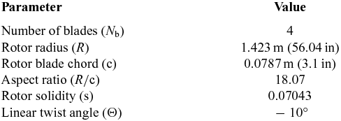
2.1 S-76 rotor geometry
The four-bladed S-76 model rotor was an 1/4.71 scale and featured − 10° of linear twist. The main characteristics of the model rotor blades are summarised in Table 2. The blade planform has been generated using eight radial stations, varying the twist Θ along the span of blade defined with zero collective pitch at the 75% R. First, the SC-1013-R8 aerofoil was used up to 18.9% R. Then, the SC-1095-R8 aerofoil from 40% R to 80% R, which covers almost half of the rotor. Finally, the SC-1095 aerofoil was used from 84% R to the tip. Between aerofoils, a linear transition zone was used. To increase the maximum rotor thrust, a cambered nose droop section was added to the SC-1095. Adding droop at the leading edge had two effects: it extended the SC1095 chord and reduced the aerofoil thickness from 9.5% to 9.4%. This section was designated as the SC-1095-R8. A detailed comparison and the aerodynamic characteristics of these aerofoils can be found in Bousman(Reference Bousman30). The planform of the S-76 model rotor with 60% taper and 35° swept tip (baseline), details on the blade radial twist, and the chord distributions are shown in Fig. 1. The thickness-to-chord ratio (t/c) is held constant and extends at almost 60% of the blade.

Figure 1. Geometry of the S-76 model rotor with 60% taper-35° swept tip, (I) SC-1094-R8 section. (II) SC-1095 section. (III) Planform. (IV) Twist distribution (Reference Balch, Saccullo and Sheehy3).
Table 2 Rotor characteristics of the 1/4.71 scale S-76 rotor blade(Reference Balch and Lombardi5)

Figure 2 shows the main geometric properties of the tips employed by Balch and Lombardi(Reference Balch and Lombardi5). The three blade tips considered here for simulations were rectangular, 60% taper 35° swept, and 60% taper-35° swept-20° anhedral. Flat and rounded tip-caps were also considered to study the effect of the formation of the tip vortex on the hover efficiency. For the round tip, two steps were taken to generate a smooth tip-cap surface. First, a small part of the blade was cut off at 1/2 of the maximum t/c (which is 9.5%) of the tip aerofoil. After this, the upper and lower points of the aerofoil were revolved about each midpoint of the section. Following this procedure, the radius of the blade did not suffer a significant change, changing originally from 56.04 inches to 56.03 inches. Figure 3 shows a view of the S-76 model rotor with 60% taper-35° swept-20° anhedral with (a) flat and (b) rounded tip-caps installed. The 20° of anhedral were introduced following the report of Balch and Lombardi(Reference Balch and Lombardi5).

Figure 2. Rotor tip configuration of the S-76 model rotor(Reference Balch, Saccullo and Sheehy3).

Figure 3. Planform of the S-76 model rotor with 60% taper-35° -20° anhedral tip, showing the details of the geometry of the flat/rounded tips.
2.2 S-76 rotor mesh
As the S-76 is a four-bladed rotor, only a quarter of the domain was meshed (see Fig. 4(b)), assuming periodic conditions for the flow in the azimuthal direction. If the wake generated by the rotor is assumed to be steady, the hover configuration can be seen as a steady problem. A C-topology around the leading edge of the blade was selected, whereas an H-topology was employed at the trailing edge of the blade. This configuration permits an optimal resolution of the boundary layer due to the orthogonality of the cells around the surface blade. Table 3 lists the grids employed for this study, showing the main meshing parameters and point distributions over the surface blade.

Figure 4. View of cross-section of the S-76 rotor mesh and boundary conditions of the background mesh.
Table 3 Meshing parameters for the S-76 mesh rotor blade
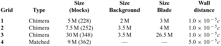
c = Rotor blade chord (3.1 inches); M = million cells (per blade)
The first cell normal to the blade was set to 7.87 × 10⁻⁷m (1.0 × 10⁻⁵ c) and 3.96 × 10⁻⁶m (5.0 × 10⁻⁵ c) for the overset and matched grid, respectively, which assures y + less than 1.0 all over the blade for the employed Re. In the chord-wise direction, between 235 and 238 mesh points were used, whereas in the span-wise direction, 216 mesh points were used. A blunt trailing edge was modelled using 42 mesh points. Figure 4(a) shows the C-H multi-block topology of the chimera mesh around the S-76 model rotor at 75%R. The computational domain with the boundary condition employed is depicted in Fig. 4(b). For all cases, the position of the far-field boundary was extended to 3R (above) and 6R (below and radial) from the rotor plane, which assures an independent solution with the boundary conditions employed. To apply periodicity at the symmetry plane, the rotor hub was approximated as a cylinder extending from inflow to outflow with a radius corresponding to 2.75% of the rotor radius R, providing a flow blockage in the root region. If the overset method is employed, a Cartesian mesh is used as background to control the refinement of the wake region with a cell spacing of 0.05c in the vertical and radial directions.
2.3 Test conditions and computations
Table 4 summarises the conditions for each tip configuration, tip Mach numbers, collective pitch settings, and employed grids. The tip Reynolds numbers at tip Mach numbers of 0.55, 0.60 and 0.65 were set to 1.00 × 10⁶, 1.09 × 10⁶ and 1.18 × 10⁶, respectively. The values of the freestream pressure and density correspond to the International Standard Atmosphere (ISA) at sea level (T = 15.0°C).
Table 4 Computational cases for the 1/4.71 scale S-76 rotor

R = Rectangular; ST = Swept-Taper; SST = Shear Stress Transport; STA = Swept-Taper-Anhedral; f = flat tip-caps; k = turbulent kinetic energy in k-ω model; r = rounded tip-caps; ω = Specific dissipation in k-ω model.
3.0 CFD METHOD
3.1 HMB2 solver
The Helicopter Multi-Block (HMB2)(Reference Lawson, Steijl, Woodgate and Barakos31-Reference Steijl, Barakos and Badcock34) code is used as the CFD solver for the present work. It solves the Navier-Stokes equations in integral form using the arbitrary Lagrangian Eulerian (ALE) formulation, first proposed by Hirt(Reference Hirt, Amsten and Cook35), for time-dependent domains, which may include moving boundaries. The unsteady Reynolds-averaged Navier-Stokes equation is discretised using a cell-centred finite volume approach on a multi-block grid. The spatial discretisation of these equations leads to a set of ordinary differential equations in time,
 $$\begin{equation}
\frac{d}{dt} ({\bf w}_{i,j,k} V_{i,j,k}) = - {\bf R}_{i,j,k} ({\bf w}),
\end{equation}$$
$$\begin{equation}
\frac{d}{dt} ({\bf w}_{i,j,k} V_{i,j,k}) = - {\bf R}_{i,j,k} ({\bf w}),
\end{equation}$$
where i, j, k represent the cell index, w and R are the vector of conservative variables and flux residual, respectively, and V i, j, k is the volume of the cell i, j, k. The upwind scheme of Osher and Chakravarthy(Reference Osher and Chakravarthy36) is used to discretise the convective terms in space, whereas viscous terms are discretised using a second-order central differencing spatial discretisation. The Monotone Upstream-centred Schemes for Conservation Laws (MUSCL) by Leer(Reference van Leer37) are used to provide third-order accuracy in space. The HMB2 solver uses the alternative form of the van Albada limiter(Reference van Albada, van Leer and Roberts38) in regions where large gradients are encountered mainly due to shock waves, avoiding non-physical spurious oscillations. An implicit dual-time stepping method is employed to performed the temporal integration, where the solution is marching in pseudo-time iterations to achieve fast convergence, which is solved using first-order backward differences. The linearised system of equations is solved using the Generalised Conjugate Gradient method with a Block Incomplete Lower-Upper (BILU) factorisation as a pre-conditioner(Reference Axelsson39). Because implicit schemes require small CFL during early iterations, some explicit iteration using the forward Euler method or the four stage Runge-Kutta method (RK4) by Jameson(Reference Jameson, Schmidt and Turkel40) should be computed to smooth out the initial flow. Multi-block structured meshes are used with HMB2, which allow an easy sharing of the calculation load for parallel job. ICEM-Hexa™ of ANSYS is used to generate the mesh.
3.2 Turbulence models
Various turbulence models are available in the HMB2 solver, which includes several one-equation, two-equation, and four-equation turbulence transition models. Furthermore, Large-Eddy Simulation (LES), Detached-Eddy Simulation (DES) and Delay-Detached-Eddy Simulation (DDES) options are also available. For this study, two equations models were employed using the Shear-Stress Transport (SST) k-ω turbulence model of Menter(Reference Menter41).
4.0 S-76 SCALE-MODEL ROTOR BLADE
4.1 Swept tip (tip Mach number of 0.65)
4.1.1 Mesh convergence
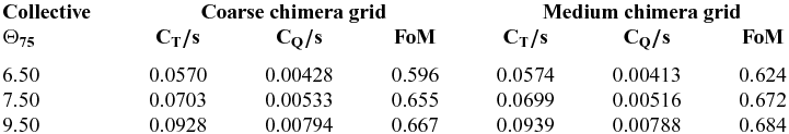
The effect of the mesh density on the FoM and torque coefficient CQ as a function of the blade loading coefficient CT/s is depicted in Fig. 5. For the foreground mesh, refinements of the boundary layer, surface tip region, and wake of the blade were carried out. However, the capability to resolve the vortex structure at the background level is key for accurate predictions of the loading on the blade. Therefore, a half million cells were added to the new background mesh (grid 2 on Table 3). The finest mesh shows a better agreement at low, medium, and high thrust coefficients with the test data of Balch and Lombardi(Reference Balch and Lombardi5). Table 5 shows the effect of the mesh density on CT/s, CQ/s, and FoM for the coarse and medium chimera grids, at blade collective angles Θ75 of 6.5°, 7.5° and 9.5°. Even though the thrust coefficient was not trimmed, less than 1.1% discrepancy was found between the employed grids. A higher FoM was obtained (4.61%, 2.61% and 2.45% for Θ75 6.5°, 7.5° and 9.5°, respectively) as result of the lower torque coefficient when the medium chimera grid was used. So the 7.5 million cells mesh was used for calculations with chimera, while 9 million cells were needed for a matched mesh.

Figure 5. Effect of the mesh density on the (a) CT/s versus FoM and (b) CT/s versus CQ for the S-76 model rotor with 60% taper-35° swept tip, Mtip = 0.65, Retip = 1.18 × 10⁶, Θ75 = 6.5°, 7.5° and 9.5°. Menter’s SST model was employed as turbulence closure. Grids 1 and 2 (see Table 3) were used.
Table 5 Effect of the mesh density on the CT/s, CQ/s and FoM for the coarse and medium chimera grids (See Table 3)

To assess the effect of using rounded tip-caps on the hover efficiency, the medium chimera grid (grid 2 on Table 3) at collective pitch 7.5° was selected for computations. Comparisons with the flat tip-caps shows a weak effect on the loading of the blade. If the flat tip-caps are taken as reference, differences of − 0.54%, − 1.01%, and 0.19% in CT/s, CQ/s, and FoM were found when the rounded tip-caps were used. In contrast, the formation of the tip vortex is completely different, which is shown in Fig. 6 through contours of vorticity magnitude at the tip blade.

Figure 6. Formation of the tip vortex on the S-76 model rotor with 60% taper-35° swept (a) flat and (b) rounded cap-tips, coloured by vorticity. Mtip = 0.65, Retip = 1.18 × 10⁶, Θ75 = 7.5°. Menter’s SST model was employed as turbulence closure. Grid 2 (see Table 3) was used.
4.1.2 Integrated loads
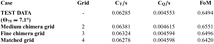
As shown in Fig. 5, the performance of the S-76 with 60% taper and 35° swept tip is well predicted with the medium chimera grid 2, which has 7.5 million cells per blade (see Table 3). Taking as baseline this tip configuration, the capability of the HMB2 solver can be explored. Predictions of the performance of the blade rotor for a large range of collective pitch angles using chimera and matched grids are evaluated. Figures 7(a) and (b) show the variation of the FoM and torque coefficients with the blade loading coefficient (black squares), respectively, at eight collective angles, which cover low, medium, and high thrust. Comparison with experimental data and momentum-based estimates of the FoM are also included in Fig. 7, using an induced power factor ki of 1.1 and overall profile drag coefficient C D0 of 0.01, showing a wrong tendency of the power divergence at high trust mainly due to flow separation(Reference Brocklehurst42). Experimental and numerical curves were established by second-order least-squares. It can be seen that the CFD computations are in close agreement with the experimental data. At low thrust, experiments and predictions show low values of the FoM, which is due to the high contribution of the profile drag. At the same test conditions, and for a collective pitch of 7°, the use of a finer chimera grid and a matched grid were investigated. The solution using the finest chimera grid 3 (right triangle in Fig. 7) has a slight effect on the FoM with respect to the computation on the medium chimera grid 2. In fact, this supports the selection of the medium chimera grid 2 to evaluate the entire range of collective pitch angles at a reduced computational cost. The effect of using a matched grid 4 is also reported in Fig. 7 (gradient symbol).

Figure 7. (a) Figure of Merit versus blade loading coefficient, (b) Torque coefficient versus blade loading coefficient, (c) Blade loading coefficient versus blade collective angle and (d) Torque coefficient versus blade collective angle for the S-76 model rotor with 60% taper-35
o
degrees swept tip,
 $M_{tip} = 0.65,\\ Re_{tip} = 1.18\times10^{6}, \Theta_{75}=4^{\circ},5^{\circ},6^{\circ}, 7^{\circ}, 8^{\circ}, 9^{\circ}, 10^{\circ}$
and 11°, k-ω SST turbulence model. Grids 2,3 and 4 (see Table 3) were used.
$M_{tip} = 0.65,\\ Re_{tip} = 1.18\times10^{6}, \Theta_{75}=4^{\circ},5^{\circ},6^{\circ}, 7^{\circ}, 8^{\circ}, 9^{\circ}, 10^{\circ}$
and 11°, k-ω SST turbulence model. Grids 2,3 and 4 (see Table 3) were used.
Table 6 summarises the S-76 (baseline) hover performance at a collective pitch of 7° using different grids and methods. The FoM performed by the medium chimera grid is predicted to within 1 counts, whereas matched and fine chimera grid predicted to within 0.7 and 0.02 counts, respectively. Figures 7(c) and (d) show the blade loading and torque coefficients as a function of the blade collective angle. Thrust and torque are slightly over and under-predicted for high collective pitch angles. This can be related to the accuracy of the experimental measurements of the blade angle or the lack of grid resolution for the blade mesh.
Table 6 Comparison between experimental data(Reference Balch and Lombardi5,Reference Balch and Lombardi6) and CFD predictions for the 1/4.71 scale S-76 rotor (baseline) at tip Mach number of 0.65 and collective pitch angle of 7°. Medium and fine chimera and matched grids were used

4.1.3 Sectional loads
Figure 8 shows the distribution of sectional thrust and torque coefficients along the rotor radius for collective pitch angles of 4° to 11°. Both coefficients are normalised with the rotor solidity s. For all collective pitch angles, a gradual increase in loading distribution is found 20%R from to 80%R, which covers half of the rotor. Note that the peak value of sectional thrust and torque coefficients were reached at 0.95R. The influence of the tip vortex on the tip region, from 95%R to 100%R, is also visible in terms of loading and torque coefficients. As a means of comparing the effect of the thrust coefficient on the tip-loss, a tip-loss factor B is computed. Tip-loss factors
 $B\approx 1-\frac{\sqrt{C_T}}{N_b}$
for the lower and higher thrust coefficient (Θ75 = 4° and 11°) were 0.9882 and 0.9781, respectively.
$B\approx 1-\frac{\sqrt{C_T}}{N_b}$
for the lower and higher thrust coefficient (Θ75 = 4° and 11°) were 0.9882 and 0.9781, respectively.

Figure 8. Blade section (a) thrust and (b) torque coefficient normalised by the rotor solidity for the S-76 model rotor with 60% taper-35° swept tip, Mtip = 0.65, Retip = 1.18 × 10⁶, and Θ75 = 4°, 5°, 6°, 7°, 8°, 9°, 10° and 11°. Menter’s SST model was employed as turbulence closure. Grid 2 (see Table 3) was used.
4.1.4 Surface pressure predictions
The surface pressure coefficient is analysed for all collective pitch angles at four radial stations along the S-76 blade on the medium chimera grid. The surface pressure coefficient is computed based on the local velocity at each radial station:
 $$\begin{equation}
C_p=\frac{p-p_{\infty }}{1/2 \rho (\Omega r R)^2}
\end{equation}$$
$$\begin{equation}
C_p=\frac{p-p_{\infty }}{1/2 \rho (\Omega r R)^2}
\end{equation}$$
Figure 9 shows the chord-wise pressure coefficient at inboard (r = 0.40), medium (r = 0.75), and outboard (r = 0.95 and 0.975) blade sections, where the critical Cp is also given to asses the sonic region of the blade (local flow above Mach number 1). It is clear that at r = 0.40 and 0.75, for all collectives, the suction peak does not exceeded the critical Cp values. By contrast, the most outboard sections (r = 0.95 and 0.975) reach sonic conditions above rotor collective angles of 7° and 5°, respectively, which lead to increased drag coefficient. This zone is clearly extended further along the blade span as the collective is increased. Despite the use of the swept tip, a mild shock is found at the vicinity of the tip. Figure 10(a) shows contours of Mach number on plane extracted at r = 0.975 for a blade collective angle of 7°, which reveals a weak shock wave. Moreover, for each blade collective angle, Fig. 10(b) shows the radial location where the local flow becomes supersonic.

Figure 9. Surface pressure coefficient at (a) r = 0.40, (b) r = 0.75, (c) r = 0 .95 and (d) r = 0.975 for the S-76 model rotor with 60% taper-35° swept tip, Mtip = 0.65, Retip = 1.18 × 10⁶, and Θ75 = 4°, 5°, 6°, 7°, 8°, 9°, 10° and 11°. Menter’s SST model was employed as turbulence closure. Grid 2 (see Table 3) was used.

Figure 10. (a) Contours of Mach number on a plane extracted at r = 0.975 for the S-76 model rotor with 60% taper-35° swept tip at blade collective angle of 7.0° and (b) Radial location where the local flow becomes first supersonic as function of the blade collective angle Θ75. For computations Mtip = 0.65, Retip = 1.18 × 10⁶ were set. Menter’s SST model was employed as turbulence closure. Grid 2 (see Table 3) was used.
4.1.5 Trajectory and size of the tip vortex
To ensure realistic predictions of the wake-induced effects, the radial and vertical displacements, and size of the vortex core should be resolved, at least for the first and second wake passages. Figure 11(a) shows a comparison of the radial and vertical displacements of the tip vortices, as functions of the vortex age (in degrees), with the prescribed wake-models of Kocurek(Reference Kocurek and Tangler43) and Landgrebe(Reference Landgrebe44). It should be mentioned that a blade loading coefficient CT/s = 0.06381 was selected, which corresponds to 7° of blade collective angle. Both empirical models are based on flow visualisation studies of the rotor wake flow, which is related to the geometric rotor parameters like the number of blades, aspect ratio, chord, solidity, thrust coefficient, and linear twist angle. The prediction of the trajectory, which is captured up to 3-blade passages (wake age of 270° for a four-bladed rotor) is in good agreement with both empirical models. The effect of the collective pitch angle (Θ75 = 5.0°, 7.0° and 9.0°) on the trajectory of the tip vortex is also investigated and is depicted in Fig. 11(b). Until the first passage (wake age of 90°), a slow convection of the tip vortices is seen in vertical displacement (–z/R). As result of the passage of the following blade, a linear increment of the vertical displacement of the wake is found, mainly due to the change in the downwash velocity. As the thrust coefficient is increased, a more rapid vertical displacement is seen for the tip vortices. On the other hand, the radial displacement is less sensitive to changes on the collective pitch angles, reaching asymptotic values approximately at r = 0.8 (see Fig. 11(b)).

Figure 11. Tip vortex displacements versus wake age (in degrees) at collective pith angles of (a) 7.0° and (b) 5.0°, 7.0° and 9.0° for the S-76 model rotor with 60% taper-35° swept tip, Mtip = 0.65, and Retip = 1.18 × 10⁶. Menter’s SST model was employed as turbulence closure. Grid 2 (see Table 3) was used.
Likewise, the vortex core size based on vorticity magnitude at collective pitch angles of Θ75 = 5.0°, 7.0°, and 9.0° were computed. Figure 12 presents the growth of the vortex core radius normalised by the equivalent chord (ce = 3.071in):
 $$\begin{equation}
c_e = 3\int _{o}^{1} c(r)\,r^2\,dr
\end{equation}$$
$$\begin{equation}
c_e = 3\int _{o}^{1} c(r)\,r^2\,dr
\end{equation}$$

Figure 12. Size of the vortex core versus wake age (in degrees) at collective pith angles of 5.0°, 7.0° and 9.0° for the S-76 model rotor with 60% taper-35° swept tip, Mtip = 0.65, and Retip = 1.18 × 10⁶. Menter’s SST model was employed as turbulence closure. Grid 2 (see Table 3) was used.
A rapid growth of the radius of the tip vortex is seen, as function of the wake age. Up to the first passage (wake age of 90°), a moderate effect of the collective pitch angles on the core size of the vortex wake is also observed, with cores reaching three times their initial values. Therefore, for the third passage (wake age of 270), the values of the core reached four times their initial value. This rapid growth it due to numerical diffusion and grid density effects.
Visualisation of the vortex flow of the S-76 rotor using the Q criterion by Jeong(Reference Jeong and Hussain45) is given in Fig. 13. For this study, the formation of the wake behind the rotor disk, is analysed using the medium and fine chimera grids, which have 7.5 and 30 million cells per blade, respectively. The collective pitch angle was set to 7.0°. For both cases, the first and second passages of the vortex are preserved. A root vortex is also predicted.

Figure 13. Visualisation of the S-76 model wake in hover using ‘Q’ criterion of 0.001 (a) Medium chimera grid 2 and (b) fine chimera grid 3. Mtip = 0.65, Θ75 = 7°, Retip = 1.18 × 10⁶, k-ω SST turbulence model. Grids 2 and 3 (see Table 3) were used.
4.2 Swept tip (tip Mach numbers of 0.55 and 0.60)
Hover predictions on the S-76 with 60% taper-35° swept flat tip at tip Mach numbers of 0.55 and 0.60 were performed at four collective pitch angles (6°, 7°, 8° and 9°). The Reynolds numbers based on the tip Mach numbers were set to 1.00 × 10⁶ and 1.09 × 10⁶, respectively. For this section, integrated performance is evaluated using the available experimental data. The medium chimera grid 2 was used as consequence of its good performance obtained previously at tip Mach number of 0.65, and its low computational cost.
4.2.1 Integrated loads
Figures 14 and 15 show the FoM and torque coefficients at tip Mach numbers of 0.60 and 0.55, respectively, as a function of the blade loading coefficient CT/s, which covers low and medium thrust. Comparisons with the momentum-based estimation of the FoM are also given, with induced power factor ki of 1.1 and overall profile drag coefficient C D0 of 0.01. It is seen that the CFD predictions slight over-predict the values of FoM at blade collective angles of 8° and 9°. Nevertheless, the calculations show a reliable correlation to overall performance, where the tip Mach number effect is well captured.

Figure 14. (a) Figure of Merit versus blade loading coefficient, (b) Torque coefficient versus blade loading coefficient for the S-76 model rotor with 60% taper-35° swept tip, Mtip = 0.60, Retip = 1.09 × 10⁶, Θ75 = 6°, 7°, 8° and 9°, k-ω SST turbulence model. Grid 2 (see Table 3) was used.

Figure 15. (a) Figure of Merit versus blade loading coefficient, (b) Torque coefficient versus blade loading coefficient for the S-76 model rotor with 60% taper-35° swept tip, Mtip = 0.55, Retip = 1.0 × 10⁶, Θ75 = 6°, 7°, 8° and 9°, k-ω SST turbulence model. Grid 2 (see Table 3) was used.
4.3 Rectangular and anhedral tips
4.3.1 Rectangular tip (tip Mach numbers of 0.60 and 0.65)
The effect of the rectangular tip on the rotor performance of the 1/4.71 scale S-76 is evaluated here. Figures 16 and 17 show the FoM and torque coefficients for collective angles from 4° to 8° and 6.5°, 7.5° and 8.5° at tip Mach numbers of 0.65 and 0.60, respectively. Comparisons with the momentum-based estimation of the FoM are also given with induced power factor ki of 1.15 and overall profile drag coefficient C D0 of 0.01. Note that rectangular tips present a higher induced power factor, leading to decrease the FoM. At tip Mach number of 0.65, it can be seen that CFD predictions over-predict the values of FoM at collective pitch angles of 7° and 8°. However, CFD results for performance at tip Mach number of 0.60 reveal a good agreement with the experimental data. For this case, the effect of using rounded tip-caps (gradient symbols in Fig. 17) was also evaluated, showing a weak effect on the FoM. The CFD results were able to predict the trend of the rectangular tip and indicate that this shape is of lower performance than the swept-tapered one.

Figure 16. (a) Figure of Merit versus blade loading coefficient, (b) Torque coefficient versus blade loading coefficient for the S-76 model rotor with rectangular flat tip, Mtip = 0.65, Retip = 1.18 × 10⁶, Θ75 = 4°, 5°, 6°, 7° and 8°, k-ω SST turbulence model. Grid 2 (see Table 3) was used.

Figure 17. (a) Figure of Merit versus blade loading coefficient, (b) Torque coefficient versus blade loading coefficient for the S-76 model rotor with rectangular flat tip, Mtip = 0.60, Retip = 1.09 × 10⁶, Θ75 = 6.5°, 7.5° and 8.5°, k-ω SST turbulence model. Grid 2 (see Table 3) was used.
4.3.2 Anhedral tip (tip Mach number of 0.60 and 0.65)
FoM and torque coefficients as function of the blade loading coefficient, for the S-76 model rotor with 60% taper-35° swept-20° anhedral tip, are given in Figs 18 and 19 at tip Mach number 0.65 and 0.60, respectively. Collective pitch angles were set to 6.5°, 7.5° and 9.5°. Comparisons with the momentum-based estimation of the FoM are also shown with induced power factor ki of 1.1 and overall profile drag coefficient C D0 of 0.01. Rounded tip-caps were computed at collective pitch of 7.5°.

Figure 18. (a) Figure of Merit and (b) Torque coefficient versus blade loading coefficient CT/s for the S-76 model rotor with 60% taper-35° swept-20° anhedral flat and rounded tips, Mtip = 0.65, Retip = 1.18 × 10⁶, Θ75 = 6.5°, 7.5° and 9.5°, k-ω SST turbulence model. Grid 2 (see Table 3) was used.

Figure 19. (a) Figure of Merit and (b) Torque coefficient versus blade loading coefficient CT/s for the S-76 model rotor with 60% taper-35° swept-20 degrees anhedral flat and rounded tips, Mtip = 0.60, Retip = 1.09 × 10⁶, Θ75 = 6.5°, 7.5° and 9.5°, k-ω SST turbulence model. Grid 2 (see Table 3) was used.
As shown for the S-76 60% taper-35° swept tip, the effect of rounding is weak. Overall, the CFD predictions are in good agreement with the experimental data at low, medium and high thrust. The results for this tip, broadly follow the swept-tapered tip trends. The main difference is the higher FoM that is obtained due to the additional off-loading of the tip provided by the anhedral. This is a known effect(Reference Brocklehurst and Barakos1) and is captured accurately by the present computations.
4.4 Comparison of surface pressure
Figure 20 shows a comparison of surface pressure for the 1/4.71 scale S-76 rotor with rectangular, swept-taper and anhedral tip configurations. This study corresponds to a medium blade loading case (CT/s = 0.06) with a tip Mach number of 0.65. Until 0.85 R, the distribution of the surface pressure for the three shapes is similar. On the other hand, a different pressure suction distribution is seen at the tip region (from 0.95 R to 1.0 R) for each blade. The suction peak distribution for the rectangular tip presents a severe reduction mainly due to compressibility effects. By contrast, the swept-taper and anhedral tips show a smoother distribution of the suction peak as consequence of the swept configuration.

Figure 20. Comparison of surface pressures for the 1/4.71 scale S-76 rotor with rectangular, swept-taper, and anhedral tip configurations for the same blade loading coefficient CT/s = 0.06. The tip Mach number was set to 0.65. The medium chimera grid was used (See Table 3).
4.5 Hovering endurance of the S-76 scale-model rotor blade
As a means of comparing the effect of the tip configuration on the 1/4.71 scale S-76 rotor in hover, hovering endurance has been estimated using the experimental data from Balch and Lombardi(Reference Balch and Lombardi5,Reference Balch and Lombardi6) and CFD predictions from HMB2. This parameter evaluates the performance capabilities of a helicopter in hover configuration, typically for a range of thrust coefficient from maximum takeoff gross to empty weight. Following Makofski(Reference Makofski46), the hovering endurance of a helicopter is given by:
 $$\begin{equation}
E\,=\,\frac{550}{(sfc) (\Omega R)} \int _{C_{T,f}}^{C_{T,i}} \frac{dC_T}{C_Q}
\end{equation}$$
$$\begin{equation}
E\,=\,\frac{550}{(sfc) (\Omega R)} \int _{C_{T,f}}^{C_{T,i}} \frac{dC_T}{C_Q}
\end{equation}$$
where sfc is the specific fuel consumption given in (lb/(rotor hp)/hr), whereas the rotor angular velocity Ω and rotor radius R have unit of rad/s and feet, respectively. For this study, the sfc is assumed to be a constant value equal to 1, and the tip Mach number was set to 0.65. The initial and final thrust coefficient corresponds to empty weight 3,178kg (CT/s = 0.04923) and maximum takeoff gross weight 5,306kg (CT/s= 0.08220) of the modern S-76 C++ helicopter.
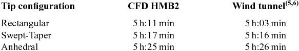
Table 7 compares the hovering endurance in hours for three tip configurations (rectangular, swept-taper and anhedral) using the available experimental data from Balch(Reference Balch and Lombardi5,Reference Balch and Lombardi6) and CFD predictions. According to the wind-tunnel data, the rectangular tip shows the worst performing blade and the swept-tapered with anhedral the best. In fact, the use of advanced tip configurations like swept-taper or anhedral has a clear benefit on the hovering endurance, delivering an extra time of 13 and 23 minutes if compared with the rectangular tip. The same trend with the shapes is captured by the present computations, which presents absolute errors of 2.57%, 0.18% and 0.55% for the rectangular, swept-taper and anhedral with respect to experiments. The good agreement of the endurance is a reflection of the accurate FoM predictions with 0.1 count.
Table 7 Effect of the tip shape on the hovering endurance (in hours) for the 1/4.71 scale S-76 main rotor at tip Mach number of 0.65
5.0 AEROACOUSTIC STUDY OF THE S-76 SCALE-MODEL
The Helicopter Ffowcs Williams-Hawkings (HFWH) code is used here to predict the mid and far-field noise on the 1/4.71 scale S-76 main rotor. This method solves the Farassat 1A formulation (also known as retarded-time formulation) of the original Ffowcs Williams-Hawkings FW-H equation(Reference Ffowcs-Williams and Hawkings47), which is mathematically represented by
 $$\begin{eqnarray}
4 \pi a_{0}^2(\rho ({\bf x},{\bf t})-\rho _0) &=& \frac{\partial }{\partial t}\int \frac{\rho _0 u_n}{r} \delta (f)\frac{\partial f}{\partial \mathrm{x_j}} \mathrm{dS(y)} -\frac{\partial }{\partial \mathrm{x_i}} \int \frac{P_{ij}}{r}\delta {(f)}\frac{\partial f}{\partial \mathrm{x_j}} \mathrm{dS(y)}\nonumber\\
&&+\,\frac{\partial ^2}{\partial \mathrm{x_i}\mathrm{x_j}} \int \frac{T_{ij}({\bf y},t-r/c)}{r} \mathrm{dV(y)} ,
\end{eqnarray}$$
$$\begin{eqnarray}
4 \pi a_{0}^2(\rho ({\bf x},{\bf t})-\rho _0) &=& \frac{\partial }{\partial t}\int \frac{\rho _0 u_n}{r} \delta (f)\frac{\partial f}{\partial \mathrm{x_j}} \mathrm{dS(y)} -\frac{\partial }{\partial \mathrm{x_i}} \int \frac{P_{ij}}{r}\delta {(f)}\frac{\partial f}{\partial \mathrm{x_j}} \mathrm{dS(y)}\nonumber\\
&&+\,\frac{\partial ^2}{\partial \mathrm{x_i}\mathrm{x_j}} \int \frac{T_{ij}({\bf y},t-r/c)}{r} \mathrm{dV(y)} ,
\end{eqnarray}$$
where Tij = ρuiuj + Pij − c 2(ρ − ρ0)δ ij is known as the Lighthill stress tensor(Reference Lighthill48), which may be regarded as an “acoustic stress”. The first and second terms on the right-hand side of Equation (5) are integrated over the surface f, whereas the third term is integrated over the volume V in a reference frame moving with the body surface. The first term on the right-hand side, represents the noise that is caused by the displacement of fluid as the body passes, which is known as thickness noise. The second term accounts for noise resulting from the unsteady motion of the pressure and viscous stresses on the body surface, which is the main source of loading, blade-vortex-interaction and broadband noise(Reference Brentner and Farassat49). If the flow-field is not transonic or supersonic, these two source terms are sufficient(Reference Brentner and Farassat49). The sound is computed by integrating the Ffowcs Williams-Hawkings equation on an integration surface placed away from the solid surface. The time-dependent pressure signal that appears in Equation (5) is obtained by transforming the flow solution from the blade reference frame to the inertial reference frame.
The HFWH requires as input the geometric location for radial sections of the rotor blade. Likewise, values of the pressure, density and three components of the velocity at the centre of each panel are required. Due to the sensitivity of the loads on the tip region (from 95%R to 100%R), a clustering of the radial sections in the span-wise direction is used.
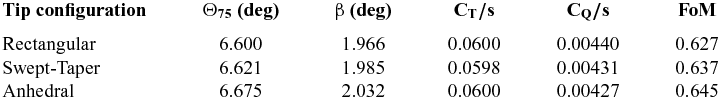
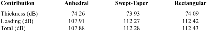
A comparative study of the effect of different tip configurations on the noise levels radiated by the scale S-76 main rotor blades was performed at tip Mach number 0.65. A trimmer state for each tip was required, being selected a medium thrust coefficient CT /σ = 0.06. Table 8 shows the blade collective angle Θ75, coning angle β, blade loading coefficient CT/s, torque coefficient normalised by the rotor solidity CQ/s, and FoM for each shape tip at the trimmer condition. The higher FoM obtained by the anhedral (1.24% and 2.83% higher than the swept-taper and rectangular tip) is due to the additional off-loading of this tip. This is a known effect reported by Brocklehurst and Barakos(Reference Brocklehurst and Barakos1).
Table 8 Performance on the 1/4.71 scale S-76 rotor with rectangular, swept-taper and anhedral tip configurations for the same blade loading coefficient CT/s = 0.06. The tip Mach number was set to 0.65. For this study, the medium chimera grid was used (see Table 3)

First, a study on the directivity of noise is investigated in the tip-path-plane of the rotor, showing the contributions of the thickness and loading noise to the total noise. The aim is to study the noise pattern at the rotor disk plane of a hovering main rotor. In hover, it is known(Reference Gopalan and Shmitz50) that the linear thickness noise dominates the in-plane acoustic at moderate tip Mach numbers (0.75 < Mtip < 0.85), whereas at lower tip Mach number, the loading noise tends to dominate(Reference Gopalan and Shmitz51). Out the rotor disk plane, the regions dominated by the loading noise correspond to a conical shape directed 30°-40° downward to the rotor disk plane(Reference Kusyumov, Mikhailov, Garipova, Batrakov and Barakos52). The second part is devoted to assess the propagation of the acoustic noise at the rotor disk plane at function of the radial distance. Moreover, comparison with the theory is also presented in terms of thickness and loading predictions.
The thickness, loading, and total noise directivity patterns are depicted in bar-chart 21 at the rotor disk plane r = 4. There is no noise directivity in this case. Table 9 summarises the contribution of thickness and loading to the total noise expressed in dB for both tip configurations. The rectangular tip presents a higher total noise (1.99dB at r = 4) with respect to the anhedral tip. It is found that rectangular and swept-taper tip provide the same total noise. Moreover, the thickness noise is not strongly affected by the used of the tip, whereas the loading noise shows larger difference.
Table 9 Thickness, loading, and total noise in the tip-path-plane of the rotor at r = 4R for the 1/4.71 scale S-76 rotor blade with rectangular, swept-tapered and anhedral tip configurations. Mtip = 0.65 and CT/s = 0.06 were used as hovering conditions


Figure 21. Thickness, loading and total noise directivity in the tip-path-plane of the rotor at r = 4 for the 1/4.71 scale S-76 rotor blade with rectangular, swept-taper and anhedral tip configurations. Mtip = 0.65 and CT/s = 0.06 were used as hovering conditions.
Due to the lack of experimental acoustic data for the S-76, a comparison with the theory was conducted in terms of thickness and loading noise predictions. Both analytical solutions are based on the work of Gopalan(Reference Gopalan and Shmitz50,Reference Gopalan and Shmitz51) and have been successfully employed in the helicopter community(Reference Kusyumov, Mikhailov, Garipova, Batrakov and Barakos52). The key idea was to convert the FW-H integral equations to an explicit algebraic expressions. In the case of the hover configuration and for an observer located at the rotor disk plane, the acoustic pressure due to blade thickness noise p′ T , is written in the form:
 $$\begin{equation}
p^{\prime }_T(\mathbf {x},t) = \frac{\rho _o a_o^2}{2}F_H F_{\epsilon } T_M ,
\end{equation}$$
$$\begin{equation}
p^{\prime }_T(\mathbf {x},t) = \frac{\rho _o a_o^2}{2}F_H F_{\epsilon } T_M ,
\end{equation}$$
where ρ o is the ambient density of air and ao is the ambient speed of sound. FH = R/rh is a distance factor, where R is the rotor radius and rH the observer distance from the rotor hub. F ε = A ε/A represents the aerofoil shape factor, where A ε is the aerofoil cross-sectional area and A is the rotor disk area. TM is the thickness factor:
 $$\begin{eqnarray}
&& T_M(\psi ,M_H)=\frac{M_{tip}^3}{12}\times \Bigg ( -\frac{(3-M_{tip} \sin \psi ) \sin \psi }{(1-M_{tip} \sin \psi )^3} +\frac{M_{tip} \cos ^2\psi }{10(1-M_{tip} \sin \psi )^4}\nonumber \\
&&\quad \times\, \Big (50+39M_{tip}^2-45M_{tip} \sin \psi -11 M_{tip}^2 \sin ^2\psi + 12M^3_{tip} \sin \psi - 18M^3_{tip} \sin ^3\psi \Big )\Bigg ) \nonumber \\
\end{eqnarray}$$
$$\begin{eqnarray}
&& T_M(\psi ,M_H)=\frac{M_{tip}^3}{12}\times \Bigg ( -\frac{(3-M_{tip} \sin \psi ) \sin \psi }{(1-M_{tip} \sin \psi )^3} +\frac{M_{tip} \cos ^2\psi }{10(1-M_{tip} \sin \psi )^4}\nonumber \\
&&\quad \times\, \Big (50+39M_{tip}^2-45M_{tip} \sin \psi -11 M_{tip}^2 \sin ^2\psi + 12M^3_{tip} \sin \psi - 18M^3_{tip} \sin ^3\psi \Big )\Bigg ) \nonumber \\
\end{eqnarray}$$
Here, ψ is the local azimuth angle and Mtip is the tip Mach number. The theoretical thickness noise mainly depends on geometric parameters of the blade. However, the effect of the tip configuration cannot be assessed by this theory.
Likewise, the acoustic pressure due to the theoretical blade loading for an observer located at the rotor disk plane can be written as
 $$\begin{equation}
p^{\prime }_L(\mathbf {x},t) = \frac{\rho _o a_o^2}{2}F_H F_T L_M ,
\end{equation}$$
$$\begin{equation}
p^{\prime }_L(\mathbf {x},t) = \frac{\rho _o a_o^2}{2}F_H F_T L_M ,
\end{equation}$$
where
 $F_T = \frac{1}{60\sqrt{2}N_b}\Big (\frac{T}{\rho _o a_o^2 A}\Big )^{3/2}$
, Nb
is the number of blades, T is the thrust, and LM
is the thrust factor:
$F_T = \frac{1}{60\sqrt{2}N_b}\Big (\frac{T}{\rho _o a_o^2 A}\Big )^{3/2}$
, Nb
is the number of blades, T is the thrust, and LM
is the thrust factor:
 $$\begin{eqnarray}
&& L_M(\psi ,M_H) = \cos \psi (1-M_{tip} \sin \psi )^{-3}\times \Bigg (60+30M_{tip}^2 \cos ^2\psi -120M_{tip} \sin \psi \nonumber\\
&&\quad -\,30M_{tip}^3\sin \psi \cos ^2\psi +80M_{tip}^2 \sin ^2\psi +9M_{tip}^4 \sin ^2\psi \cos ^2\psi -20M_{tip}^3\sin ^3\psi \Bigg )
\end{eqnarray}$$
$$\begin{eqnarray}
&& L_M(\psi ,M_H) = \cos \psi (1-M_{tip} \sin \psi )^{-3}\times \Bigg (60+30M_{tip}^2 \cos ^2\psi -120M_{tip} \sin \psi \nonumber\\
&&\quad -\,30M_{tip}^3\sin \psi \cos ^2\psi +80M_{tip}^2 \sin ^2\psi +9M_{tip}^4 \sin ^2\psi \cos ^2\psi -20M_{tip}^3\sin ^3\psi \Bigg )
\end{eqnarray}$$
Comparisons of the theoretical and numerical thickness, loading and total noise at the rotor disk plane are shown in Fig. 22, as function of the observer distance rH
. The x axis represents the observer time (
 $t=\frac{\psi +M_{tip}(\cos \psi -1)}{\Omega })$
. In the case of the S-76 at tip Mach number of 0.65, a rotor period corresponds to 0.0404s (360°).
$t=\frac{\psi +M_{tip}(\cos \psi -1)}{\Omega })$
. In the case of the S-76 at tip Mach number of 0.65, a rotor period corresponds to 0.0404s (360°).

Figure 22. Comparison of thickness, loading and total noise distribution at radial distance 2,4 and 8 in the rotor disk plane for the 1/4.71 scale S-76 rotor with rectangular, swept-taper and anhedral tip configurations. Theoretical noise by(Reference Gopalan and Shmitz50,Reference Gopalan and Shmitz51) is also shown. Mtip = 0.65 and CT/s = 0.06 were used as hovering conditions.
For all observer distances, the effect of the tip configuration on the numerical thickness noise is negligible (see Fig. 22). The numerical simulation results are in close agreement with the analytical solution, where the peak of negative pressure is well predicted by HFWH.
Figure 23(a) shows the total noise as a function of the radial distance in the rotor disk plane for each tip configuration. A least square method was employed to fit the total noise distribution. For a radial distance of 10 times the rotor radius R, the swept-tapered tip is 1.83dB louder than the anhedral in term of total noise. It has been seen that at the rotor disk plane both tip configurations generate the the same total noise, with a slight higher value for the case of the swept-taper. However, there are other regions where the contribution of the thickness and loading noise can be assessed. These contributions are shown in Table 10 for a microphones located 45° downward to the rotor disk plane. A reduction of the total noise (4.53dB) is gained if the anhedral tip configuration is used. Figure 23(b) shows the total noise as a function of the radial distance for a set of microphones located 45° downward to the rotor disk plane. It is seen than the swept-tapered tip is louder than the anhedral tip. It is mainly due to the effect of the loading noise distribution, which is the main mechanism of noise generation in this direction.

Figure 23. (a) Total noise for the 1/4.71 scale S-76 rotor blade with rectangular, swept-taper and anhedral tip configurations, as function of the radial distance in the rotor disk plane (b) Total noise as a function of the radial distance for a set of microphones located 45° downward and upward to the rotor disk plane. Mtip = 0.65 and CT/s = 0.06 were used as hovering conditions.
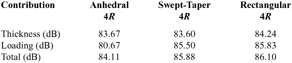
Table 10 Thickness, loading and total noise for a microphone located 45° downward to the rotor disk plane (r = 3) for the S-76 rotor blade with rectangular, swept-tapered and anhedral tip configurations. Mtip = 0.65 and CT/s = 0.06 were used as hovering conditions
6.0 FULL-SCALE S-76 ROTOR BLADE
The full-scale S-76 rotor was tested by Johnson(Reference Johnson7) in the Ames 40- × 80-foot wind tunnel for a wide range of advance ratio from 0.075 to 0.40 and an advancing side tip Mach number Mat range from 0.640 up to 0.965. The aim was to study the effect of four advanced tip geometries (rectangular, tapered, swept and swept-tapered) on the performance, blade vibratory loads and acoustic noise of the rotor. Due to secondary flow into the test chamber, rotor forces and moments (measured in the wind axis system) were corrected for wall effects and for tares, based on an incremental change in the angle-of-attack proportional to the uncorrected lift. Like the model scale, it was found that the swept tapered tip had the better performance in forward flight mainly due to a lower power required. A further discussion of the rotor performance was reported by Stroub(Reference Stroub, Rabbott and Niebanck53), whereas blade vibratory loads and noise were investigated by Jepson(Reference Jepson, Moffitt, Hilzinger and Bissell8). This campaign of test was accomplished with a comparison of the full-scale to 1/5 model-scale, flight test results and theoretical calculations conducted by Balch(Reference Balch54).
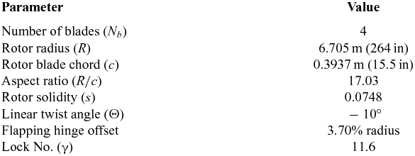
The majority of the previous experimental tests on the full-scale S-76, however, did not perform hover cases. To fill this gap, a major study to establish a database on the S-76 full scale in hover was undertaken by Shinoda(Reference Shinoda9,Reference Shinoda10) . The NASA Ames 80- × 120-foot wind tunnel was used as a hovering facility, where the S-76 rotor blade with 60% taper-35° swept tip at tip Mach number 0.604 was selected. Table 11 lists the full-scale S-76 main rotor parameters, which indicates a high Lock number of 11.6.
Table 11 Rotor characteristics of the S-76 full model rotor blade(Reference Shinoda10)
6.1 Aeroelastic analysis of the S-76 rotor
For this study, the use of a static analysis on the S-76 full-scale rotor blade with 60% taper-35° swept tip was put forward as a means to quantify its effect on the rotor performance.
6.1.1 Structural model
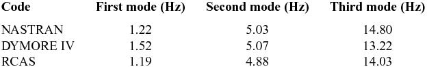
A structural model of the S-76 model was generated using the available data from Johnson(Reference Johnson7) and Jepson(Reference Jepson, Moffitt, Hilzinger and Bissell8). In Fig. 24 the blade is modelled using 17 elements of the CBEAM type of NASTRAN. Likewise, the rigid bar elements (RBAR) are also shown, which have no structural properties, and used to link the chord nodes to the leading edge with the trailing edge. Due to the distribution along the span-wise of the rotor for the Young’s modules, Poisson’s ratio and torsional stiffness were not available, the material properties of the UH-60A(Reference Hamade and Kufeld55) were used for this study. The structural properties of the blade are presented in Fig. 25, which suggests that the blade suffers a reduction of the beam-wise, chord-wise, and torsional stiffness from the normalised radial position r = 0.75 to the tip corresponding to, 78.9%, 71.0% and 86.4%. Table 12 shows a comparison of the eigenfrequency obtained using NASTRAN with DYMORE IV, and RCAS results by Monico(Reference Monico56) for the first three modes at the nominal speed of the rotor 296rpm, which suggests fair agreement.

Figure 24. Structural model of the full-scale S-76 rotor blade, showing the distribution of the 17 elements of the CBEAM type through the span-wise of the blade.

Figure 25. (a) Sectional area and linear mass distribution and (b) Chord-wise, flap-wise and torsional area moments of inertia for the S-76 rotor blade with 60% taper-35° swept tip(Reference Shinoda10).
Table 12 Eigenfrequencies of the full-scale S-76 rotor blade at nominal speed 296rpm, using NASTRAN. Comparison with the DYMORE IV and RCAS codes(Reference Monico56) is also shown
6.1.2 Analysis of elastic blade results
Numerical simulations of the full-scale S-76 with a set of rigid and elastic rotor blades were performed at tip Mach number of 0.605. For this hovering case, the tip Reynolds number was set to 5.27 × 10⁶, being 4.71 times larger than the model-scale. The importance of Reynolds number is well established in fixed wing aerodynamics. By contrast, in the case of rotary wing like the helicopters, it is still not well understood(Reference Singleton and Yeager57). Moreover, the low Reynolds number of the model-scale may cause premature separation which does not occur at full-scale as a result of the turbulent boundary layer. This effect leads to increased FoM for the full-scale rotor.
A set of collective pitch angles corresponding to low, medium, and high thrust coefficient were simulated. It is interesting to note that coning angles were set according to Shinoda’s report(Reference Shinoda10), with coincident flapping and lead-lag hinges located at 0.056R for the model rotor.
Figure 26 presents the FoM as a function of the blade loading coefficient CT/s at different collective pitch angles computed with HMB2. Comparison with the experimental data of Shinoda and Sikorsky Whirl Tower(Reference Shinoda10) is also shown. Vertical lines labeled as empty (3,177kg) and maximum gross (5,307kg) weight, define the hover of the S-76 helicopter rotor. The filled delta symbols correspond to the rigid calculations. At low and medium thrust coefficient, the prediction of the FoM between the Sikorsky Whirl Tower and CFD with rigid blade is well captured. At high thrust, however, the FoM is slightly over-predicted. On the other hand, the FoM is over-predicted if compared with the experimental data of Shinoda. The reason for this disagreement may be partly due to the variations in experimental data between Sikorsky Whirl Tower and wind tunnels. The reason can be due to wake reingestion as a consequence perhaps of mild in-ground effect and tunnel walls. The gradient symbols correspond to the aeroelastic calculations. It is found that at low and medium thrust coefficient C T /s = 0.031 and 0.057, the FoM does not suffer a significant change. In contrast, a better agreement between CFD and experimental data at high thrust is found. In fact, the drop in performance (3.48% of FoM at C T /s = 0.087) is a consequence of the lower twist introduced by the structural properties of the blade. The scatter of the tunnel data is remarkably large, and two lines were best-fitted corresponding to lower and upper bounds.

Figure 26. Effect of the rigid/elastic blades on the Figure of Merit for the S-76 rotor blade with 60% taper-35° swept tip, showing the experimental data of Shinoda and Sikorsky Whirl Tower(Reference Shinoda10). Mtip = 0.60 and Re tip = 5.27 × 10⁶ were set for computations. Menter’s SST model was employed as turbulence closure. Grid 2 (see Table 3) was used.
6.2 Trajectory of the tip vortex
This section shows a comparison of the radial displacements of the tip vortices as a function of the vortex age (in degrees) for the full-scale S-76 with rigid blades. Comparison with the prescribed wake model of Landgrebe(Reference Landgrebe44) and experimental data carried out by Swanson(Reference Swanson11) are also shown in Fig. 27. As it has been introduced, the flow visualisation of the rotor wake flow was performed in the NASA Ames 80- × 120-foot wind tunnel in 1993, using a shadowgraph flow visualisation technique. Two blade collective angles were selected for computations, corresponding to medium and high thrust, CT/s= 0.065 and 0.080. The prediction of the radial displacement is in good agreement with the experimental data and empirical model for both thrust coefficients. By contrast, the lack of experiments for the vertical displacement and size of the vortex core result in a deficient validation of the complete wake.

Figure 27. Comparison of the radial displacements of the tip vortices as functions of the vortex age (in degrees), with the prescribed wake-model of Landgrebe(Reference Landgrebe44) and experimental data of Swanson(Reference Swanson11) for two blade loading coefficients (a) C T /s = 0.065 and (b) C T /s = 0.080. This case corresponds to the full-scale S-76 rotor with 60% taper-35° swept tip and M tip = 0.605.
6.3 Aeroacoustic study of the full-scale S-76 rotor blade
Like the 1/4.71 scale S-76 main rotor, an aeroacoustic study of the full-scale S-76 rotor blade using the HFWH code is presented here. Comparisons of the theoretical and numerical total noise for a set of microphones located at the rotor disk plane and 45° downward and upward to the rotor disk plane are shown in Fig. 28. Despite that model-scale and full-scale rotors have different range of frequencies (higher for the model-scale), the amplitude of the sound waves should be similar for the same loads. Figure 28(a) shows an excellent agreement with the theory for all radial distances. Moreover, Fig. 28(b) shows that the total noise has the same trend downward and upward to the rotor disk plane.

Figure 28. (a) Total noise for the full-scale S-76 rotor blade with swept-taper tip configuration, as function of the radial distance in the rotor disk plane (b) Total noise as a function of the radial distance for a set of microphones located 45° downward and upward to the rotor disk plane. Mtip = 0.60 and CT/s = 0.057 were used as hovering conditions.
7.0 COMPARISON BETWEEN FULL AND MODEL-SCALE ROTORS
This section presents a comparison between the full- and model-scale S-76 rotors in terms of FoM. When comparing model-scale to full-scale rotor performance data, some considerations should first be made. First, the full-scale tip Mach number must be matched. Thus, the rotational velocity of the model-scale rotor would be multiplied by a geometric scale factor (4.71 for the S-76 rotor). Second, the Reynolds number is not possible to match if the full-scale tip Mach number is kept constant for both rotors. This parameter is the main cause of differences between full-scale and model-scale rotor test data. Finally, the rotor blade elasticity should also be considered at high thrust to fully model the blade structural aeroelasticity effects.
Figure 29 shows the effect of the Reynolds number on the FoM for the S-76 rotor blade with 60% taper-35° swept tip. Experimental data correspond to the Sikorsky Whirl Tower(Reference Shinoda10) for the full-scale rotor (solid line), and Balch and Lombardi(Reference Balch and Lombardi5) for the model-scale rotor (dashed line), where the tip Mach number was set to 0.60. CFD results are represented by triangles and squares for the full-scale (elastic blades are considered) and model-scale, respectively. Analysing the experimental data, a higher FoM is observed for the full-scale rotor over the whole range of thrust coefficient. For instance, the FoM is 6.26% higher for a medium thrust coefficient (CT/s = 0.060) and 9.66% higher for a high thrust coefficient (CT/s = 0.092). This is consistent with experience, and justified by the decrease of the aerofoil drag coefficient for increasing Reynolds number. This is also shown for the aerofoils of the S-76 rotor blade by Yamauchi(Reference Yamauchi and Johnson58), p. 30. This behaviour is also observed in the CFD results, which confirms that the present method is able to capture the Reynolds number effects.

Figure 29. Effect of the Reynolds number on the Figure of Merit for the S-76 rotor blade with 60% taper-35° degrees swept tip, showing the experimental data of Sikorsky Whirl Tower(Reference Shinoda10) (full-scale) and Balch and Lombardi(Reference Balch and Lombardi5,Reference Balch and Lombardi6) (model-scale). CFD results correspond to Mtip = 0.60 and Re tip = 5.27×10⁶and1.09×106 for the full-scale and model-scale, respectively. Menter's SST model was employed as turbulence closure. Grid 2 (see Table 3) was used.
8.0 CONCLUSIONS AND FUTURE WORK
In this paper, predictions from the CFD code HMB2 are compared against experimental data for the thrust and torque on the hovering 1/4.71 scale and full-scale S-76 main rotor. Although only integrated aerodynamic loads are available from the experiments, good agreement was found for the employed blade-tip geometries. The results highlight the advantage of Navier-Stokes CFD methods that need no assumptions regarding the tip vortex formation. The main conclusions from this work are:
-
• The effect of tip Mach and shape is captured by CFD with 0.1 counts of FoM.
-
• The anhedral was found to offer significant benefits if a modest amount is used.
-
• The acoustics in hover was also improved by the anhedral that reduced the noise by 5%.
-
• Scaled rotor performance is well predicted as loads and wake, though full-scale data are harder to reproduce and experiments show large scatter above 3 counts of FoM.
-
• CFD with modest CPU time is ready for industrial use for hover.
-
• The paper calls for full-scale tests to improve scatter in experiments and combined wake measurements with acoustic data. Measurements of surface pressure and skin friction for full-scale rotors should also be a priority.
ACKNOWLEDGEMENTS
The use of the cluster Chadwick of the University of Liverpool is gratefully acknowledged. Part of this work is funded under the HiperTilt Project of the UK Technology Strategy Board (TSB) and AugustaWestland (AW).