1. INTRODUCTION
In several research fields, such as astrophysics or inertial fusion confinement, knowledge and understanding of the interactions between photons and plasma particles, i.e., plasma optical properties, are essential (Hora, Reference Hora2007; Batani et al., Reference Batani, Dezulian, Redaelli, Benocci, Stabile, Canova, Desai, Lucchini, Krousky, Masek, Pfeifer, Skala, Dudzak, Rus, Ullschmied, Malka, Faure, Koenig, Limpouch, Nazarov, Pepler, Nagai, Norimatsu and Nishimura2007; Gonzalez et al., Reference Gonzalez, Stehle, Audit, Busquet, Rus, Thais, Acef, Barroso, Bar-Shalom, Bauduin, Kozlova, Lery, Madouri, Mocek and Polan2006; Thareja & Sharma, Reference Thareja and Sharma2006; Nardi et al., Reference Nardi, Fisher, Roth, Blazevic and Hoffmann2006; Hoffmann et al., Reference Hoffmann, Blazevic, Ni, Rosmej, Roth, Tahir, Tauschwitz, Udrea, Varentsov, Weyrich and Maron2005). Thus, as an example, the radiation emitted from hot plasmas or short-life plasmas could be the most important diagnostic tool, since the emitted spectrum contains information about the local instantaneous density and temperature (Salzmann, Reference Salzmann, Birman, Edwards, Friend, Llewellyn Smith, Rees, Sherrington and Veneziano1998). Therefore, plasma optical properties must be determined properly. This fact implies accurate calculations for both the atomic data and the populations of the electronic configurations involved, and that continuous efforts are made in the modeling plasmas.
Carbon is one of the most important elements under investigation, since it is likely to be a major plasma-facing wall component in the international thermonuclear experimental reactor (ITER) (Skinner & Federici, Reference Skinner and Federeci2006), and it plays a major role in inertial fusion scenarios (Filevich et al., Reference Filevich, Grava, Purvis, Marconi, Rocca, Nilsen, Dunn and Johnson2007). Therefore, radiation rates from carbon impurities must be known. Moreover, some laser experiments have focused on the spectrally resolved emission from hydrocarbon systems (Weaver et al., Reference Weaver, Busquet, Columbant, Mostovych, Feldman, Klapisch, Seely, Brown and Holland2005). Consequently, the study of carbon plasmas is a subject of current interest and many efforts are on going. In particular, recent kinetics code workshops (Bowen et al., Reference Bowen, Lee and Ralchenko2006; Rubiano et al., Reference Rubiano, Florido, Bowen, Lee and Ralchenko2007) have focused on comparisons of modeling calculations for specific cases that allow for testing the models, since there are very few experimental measurements for carbon plasmas.
For these reasons, it is interesting to characterize carbon plasmas. In this work, we study optically thin carbon plasmas under steady state conditions. Since we only consider optically thin plasmas, the mean free path of the photons is larger than the plasma dimensions, and then there is no photon reabsorption. Consequently, photoionization, photoexcitation, and stimulated emission processes have such small rates that they can be neglected. Furthermore, the steady state assumption requires that the relaxation time for important atomic processes be short compared with the time over which the macroscopic plasma parameters vary. On the other hand, as known, at very low and high densities, the collisional radiative steady state (CRSS) equations provide, respectively, the same results as those obtained from corona (C) and Saha-Boltzmann (SAHA) equations. This fact has allowed for distinguishing three regimes in the plasma: corona equilibrium (CE), local thermodynamic equilibrium (LTE), and non-local thermodynamic equilibrium (NLTE).
Optically thin plasmas achieve CE at very low density, where the collisional excitation rate is rather small in comparison with the spontaneous decay, and therefore, the population of the ground state is very high with respect to the population of the excited levels. In the limiting case, when the electron density is close to zero, the populations of ground and excited levels tend to one and zero, respectively. Moreover, the three body recombination process has a very low rate (due to the small probability of finding two free electrons nearby the ion at low density), and the dominant processes which govern the average ionization are the electron impact ionization and autoionization, as well as the radiative recombination and the electron capture. Since the contribution of the autoionization process is temperature and density independent, and the contribution of the electron impact ionization decreases as the density does, the autoionization results is a very important ionization mechanism in the CE regime.
The LTE regime is attained at high density and it requires that the collisional excitation rate be much larger than the spontaneous decay rate. On the other hand, the three-body recombination rate is bigger than the radiative recombination and electronic capture ones. Furthermore, the autoionization rate is much smaller than the electron impact ionization one. Therefore, the average ionization will be governed by three body recombination, and electron impact ionization processes. Finally, it is worth pointing out that in the LTE regime, the population of the excited states is relevant.
The main goal of this work is the determination of the average ionization and plasma regimes (CE, LTE, and NLTE), for steady state optically thin carbon plasmas, as a function of the density and temperature. In the literature, there are available some qualitative criteria to estimate when an ion or ion level can be considered under CE, NLTE, or LTE conditions (Mosher, Reference Mosher1974; Griem, Reference Griem1963; Salzman, 1998). However, we have employed another criterion that can state the regime of the whole plasma. The characterization of these regimes has an obvious interest in calculating plasma optical properties because it provides valuable information. First, the knowledge of the plasma regime for a given density and temperature conditions could entail a considerable saving in calculation time, since SAHA and CE equations are solved faster than rate equations. Moreover, this study also identifies which are the most relevant ions for each plasma condition, decreasing the number of them to be considered. This fact allows us to include more levels per ion, which is important in the determination of optical properties.
All the calculations presented in this work were performed using ABAKO, which is an improvement over the ATOM3R code (Florido et al., Reference Florido, Gil, Rodríguez, Rubiano, Martel and Mínguez2005), and it also integrates the RAPCAL code (Rodríguez et al., Reference Rodríguez, Gil, Florido, Rubiano, Martel and Mínguez2006), in order to calculate optical properties for a wide range of temperatures and electron number densities. This code is structured in three modules. The first one is devoted to the calculation of the atomic data required, for instance, the structure of different ions in the plasma, energy levels for ground and excited states, and oscillator strengths. In the second one, level populations are computed under both CE, LTE (SAHA equations), and NLTE (CRRS model) conditions. Finally, in the third module, the optical properties such as emissivity, opacity, and source function, both for LTE and NLTE situations are obtained making use of the outputs of the two previous modules.
In the next section, these modules are briefly described and will explain some of the considerations used in this work, such as the set of atomic configurations, and the calculations of their atomic magnitudes, or the model of continuum lowering. In Sections 3 and 4, results and main conclusions are presented, respectively.
2. DESCRIPTION OF THE CODE
2.1. Atomic data module
This module can work on two complementary levels depending on the atomic number or the ionization degree of the element under consideration. The first one is mainly used for low-Z or highly ionized medium and high-Z plasmas, where we used a detailed level description provided by the FAC code (Gu, Reference Gu2003), in which the bound states of the atomic systems are calculated with convenient specification of coupling schemes and including configuration mixing.
On the other hand, for lower ionized intermediate and high-Z plasmas, this detailed calculation becomes impracticable, and a detailed relativistic configuration accounting approach is chosen. Moreover, in this case, in order to avoid the iterative procedures of the self-consistent models, the atomic magnitudes are evaluated using central analytical potentials, within the framework of the independent particle model, which have demonstrated to be an interesting and useful option to work out accurate ionic populations, and average ionizations in a wide range of densities and temperatures. In particular, ABAKO works using a set of analytical potentials developed by us, which can model both isolated ions (Martel et al., Reference Martel, Doreste, Mínguez and Gil1995) and ions immersed into plasmas (Gil et al., Reference Gil, Martel, Mínguez, Rubiano, Rodríguez and Ruano2002), including plasma effects (such as the continuum lowering of the ionization potential and the shift on the energy levels, total energies and wave functions), and single and core excited configurations (Rodríguez et al., Reference Rodríguez, Rubiano, Gil, Martel and Mínguez2002a, Reference Rodríguez, Gil, Florido, Rubiano, Martel and Mínguez2002b). Even for situations wherein more celerity is desired, the code can perform the atomic calculations using a relativistic-screened hydrogenic model (Rubiano et al., Reference Rubiano, Rodríguez, Gil, Martel and Mínguez2002a, Reference Rubiano, Rodríguez, Gil, Ruano, Martel and Mínguez2002b).
The continuum lowering due to the influence of the plasma surrounding is also considered. This one can be calculated either by means of the expression due to Stewart and Pyatt (SP) or through an expression provided by the new non-isolated analytical potential (NIP) recently developed by us (Rodríguez et al., Reference Rodríguez, Gil, Florido, Rubiano, Martel and Mínguez2005). This second expression gives results similar to those obtained from the SP model.
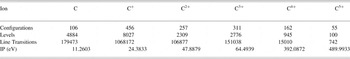
In this work, all the atomic data were obtained by using the FAC code, including configuration interaction. Thus, the total number of levels and line transitions included has been 19041 and 1521312, respectively. In Table 1, these quantities are listed for each ion stage and in Table 2, there is shown the set of configurations considered per ion following the indications given in the fourth NLTE workshop (Rubiano et al., Reference Rubiano, Florido, Bowen, Lee and Ralchenko2007). The principal quantum number n runs from 1 to 10, the orbital angular momentum l runs from 0 to 11, and l' runs from 0 to 3. Finally, the SP continuum-lowering model was used.
Table 1. List of the number of configurations, levels, bound-bound transitions, and ionization potentials used modeling carbon plasmas

Table 2. Set of configurations used for each ion stage modeling carbon plasmas
2.2. Level populations module
The calculation of ionic state distributions and level populations are performed by solving a CRSS model, both under LTE and NLTE conditions. Although the CE and SAHA equations are also implemented in this module, it was shown in a previous work (Florido et al., Reference Florido, Gil, Rodríguez, Rubiano, Martel and Mínguez2005) that levels populations obtained by solving the CRRS model are in good agreement with those predicted by SAHA and CE, at high and low electron density limits, respectively. The populations can be computed with reasonable accuracy for plasmas of any element in a wide range of conditions, both for optically thin and thick plasmas (Mínguez et al., Reference Mínguez, Rodríguez, Gil, Sauvan, Florido, Rubiano, Martel and Mancini2005). In the last case, the radiation transport is modeled through the escape factor formalism (Mancini et al., Reference Mancini, Joyce and Hooper1987). The processes included in the CRSS model are the following: collisional excitation and desexcitation; spontaneous decay; collisional ionization and three body recombination; radiative recombination; autoionization and electronic capture, being the majority of the rate coefficients evaluated by analytical formulas that can be found in the literature. In order to solve the set of rate equations, we employed the technique of sparse matrix to store the non-zero elements. This implies substantial savings in computing time and memory requirements, and it allows us to include a large amount of ionic configurations in our calculations. On the other hand, this fact increases the system dimension, which can easily reach the order of 105 for low-Z plasmas, and the most suitable choice to carry out the matrix inversion is the iterative procedure, because it requires much less memory than direct methods and it is also faster. It is worth mentioning this last fact, because when we include plasma effects in the atomic model, there is a rise in the computational time, since this second module and the atomic one have to be solved iteratively until the convergence is achieved.
2.3. Optical properties module
The spectrally resolved and mean emissivities and opacities are determined making use of the populations and the atomic data given in the previous modules. Bound-bound opacity and emissivity are calculated by using the Voigt profile for all the lines, and assuming complete redistribution of the photons. In this Voigt profile, natural, Doppler, and Stark widths are included, using a simplified semiempirical method for obtaining the last one (Zeng & Yuan, Reference Zeng and Yuan2002). For low- and highly-ionized medium and high-Z elements, the bound-free cross section is calculated quantum mechanically. In the other cases, Kramer's formula is employed. Finally, the free-free spectrum has been obtained employing the Kramer's formula for the cross section (corrected by the gaunt factor). Both for bound-free and free-free processes, it has been assumed a Maxwell-Boltzmann distribution for the free electrons.
3. RESULTS
This section is divided into three parts: the first one is devoted to the validation of our calculations for the continuum lowering and average ionization. In the second, the analysis for the average ionization and the determination of the plasma regime depending on the plasma conditions is given. Finally, in the third part, a brief comparison of the radiative properties under CE, LTE, and NLTE approaches is performed.
As our study covers a wide range of densities, it is necessary to employ a model including continuum lowering in the calculations at high density. In this work, we have chosen the SP model. In order to test it, we have plotted in Figure 1, the continuum lowering for He-like carbon ions, under different plasma conditions, calculated with different theoretical models (SP, NIP, and ion-sphere (IS) models), along with results obtained in the experiments carried out by Maksimchuck et al. (2000) with 100-fs laser pulses. The plasma density varies from 1021 to 5 × 1022 cm−3 and temperature is very close to 75 eV. For these conditions, the energy shift due to the continuum lowering is about 10%. A good agreement between the SP and the experimental results is found and a reasonable concurrence is observed between SP and those provided by the analytical potential including plasma effects NIP.

Fig. 1. Continuum lowering supplied by different theoretical models and by the experiment for He-like carbon ion versus time evolution of the plasma. Enclosed there are listed the density and temperature conditions corresponding to each time value.
In Table 3, we show the average ionization, calculated with and without continuum lowering, and the relative deviations between them. As it was expected, the average ionization is larger when including the continuum lowering. The deviations rise as the density increases and temperature decreases. Thus, we have obtained relative deviations of about 1% at 1016 cm−3 and 1 eV, at 1019 cm−3, and 10 eV, or at 1021 cm−3 and 100 eV. However, if we increase the density by two orders of magnitude for the temperatures 1 and 10 eV, the relative deviations grow to 25% and 30%, respectively.
Table 3. Average ionization calculated with and without continuum lowering, and their relative deviations

Two situations have been distinguished when checking the average ionization: low and moderate densities, low temperatures, and high densities covering a wide range of temperatures. The first situation is illustrated in Table 4, where our results are compared with data coming from a detailed kinetics model (ATOMIC) for carbon, which assumes the fine-structure approximation including intermediate-coupling and configuration-interaction effects for atomic data, as well as quantum mechanic calculations for cross sections of the atomic processes (Colgan et al., Reference Colgan, Fontes and Abdallah2006). Table 5 shows the second situation, wherein our results are now compared with those obtained from different kinetics codes, which were presented at the third Non-LTE Code Comparison Workshop (Bowen et al., Reference Bowen, Lee and Ralchenko2006). From both tables, it is observed that our results are in general in very good agreement with the other calculations. As an example, at low temperature, the mean deviation obtained in the average ionization is around 3%.
Table 4. Average ionizations (1) calculated by ABAKO (a) and by ATOMIC (b) and their relative differences in percentage (2) at low temperatures and low and moderate densities. The mean difference in the average ionization for these cases is 3.12%

Table 5. Average ionization for a density of 1022 cm−3 and several temperatures. Comparisons among the results from ABAKO (a), ATOMIC (b) and other kinetics codes of the third NLTE Code Comparison Workshop (c-e)

Once we have checked the models employed in this work, the analysis of the average ionization is started. First, we have determined this magnitude by using ABAKO, solving the CRSS equations for plasma conditions that ranged in temperatures from 1 to 200 eV, and in densities from 1012 to 1022 cm−3, and the results are plotted in Figure 2. Quantitative results are listed in Table 6.

Fig. 2. Map of the average ionization in a wide range of electron temperature and density.
Table 6. Average ionization (Z¯CRES) obtained using ABAKO solving CRSS equations

It is shown in both Figure 2 and Table 6, that for low density (under 1016 cm−3) and temperatures above 10 eV, the average ionization does not depend sensitively on the density, and this result is expected since this region is in close proximity to the CE for carbon plasmas, as we will show later. This independence of the density is better illustrated in Figure 3, where we plotted the average ionization versus the temperature for low-density situations (from 1012 cm−3 to 1016 cm−3). Thus, for example, at 10 eV, the average ionization is 3.69, and 3.88 for densities of 1012 cm−3 and 1016 cm−3, respectively. However, at 20 eV, and for the same densities, the average ionization is 3.99 and 4, respectively. The relative difference for the first temperature is about 5%, whereas for the second temperature is reduced to 0.1%. On the other hand, in general, the average ionization increases with the temperature, and this behavior is also shown in Figure 3. Thus, for temperatures lower than 1 eV, a very small ionization is found (the neutrality is achieved for low-density plasma around 0.1 eV), whereas the opposite tendency is produced over the 100 eV (at a temperature of 150 eV, only the fully stripped ion is present in the plasma).

Fig. 3. Average ionization versus electron temperature at low densities (1012–1016 cm−3) as well as in the density range 1018–1021 cm−3.
A plateau is observed in Figure 3 for densities between 1012 and 1019 cm−3. At this plateau, the average ionization is equal to four, which means that, practically, the only ion present in the plasma is the He-like one. At low densities (under 1016 cm−3), this plateau is located at temperatures between 25 and 40 eV. Furthermore, for this region of low density, there is a window in the temperature, from 40 to 63 eV, wherein only the H- and He-like ions are present in the plasma (see Fig. 4). At 25 eV, we have just He-like ions, but at 63 eV, H and He ions are both present in the same proportion. As we said previously, in these conditions, carbon plasma is close to CE and, therefore, the emissivity will be govern mainly by the continuum spectrum, and the opacity by the Hα,β,γ and Heα,β,γ lines.

Fig. 4. He- and H-like carbon ion populations versus temperature at low densities. The populations have been obtained solving CE equations and CRSS ones at 1016 cm−3.
In order to identify the regions corresponding to CE, NLTE, and LTE situations, for optically thin carbon plasmas, we carried out our analysis focusing attention on the average ionization, and on the ion and level populations. For this purpose, we proceeded as follows: when the ion populations calculated from CE and SAHA equations present a mean deviation (Δp), with respect to those obtained from the CRSS model, larger than a certain criterion imposed (Δp*), then we consider the NLTE regime. Otherwise, we assume that CE or LTE has been achieved. The mean deviation Δp is calculated using
where i runs over the whole set of ions and k denotes either CE or SAHA. By fixing Δp* equal to 0.1 (= 10%), we obtained the map of the CE, LTE, and NLTE regions for carbon plasmas that is shown in Figure 5.

Fig. 5. Map of CE, LTE and NLTE regimes determined using ABAKO.
We have checked that this criterion ensures that the relative deviations in the average ionization, ΔZ¯ are always less than or equal to 1%, as can be verified by comparing Tables 7 and 8. Figure 6 illustrates the correct behavior of the average ionization at the limits of low and high electron density, since the CCRS results must converge to those obtained from CE and SAHA equations, respectively. Figure 6 also shows the significance of considering the continuum lowering and the autoionization process at high and low densities, respectively.

Fig. 6. Average ionization versus free electron density calculated using CRSS, SAHA, and CE equations. Dashed lines represent calculations without considering autoionization and continuum lowering.
Table 7. Relative differences in percentage between the average ionization calculated with CRSS and CE equations,ΔZ¯C, and CRSS and SAHA equations, ΔZ¯S

Table 8. Mean deviations in percentage of the ion populations calculated with CRSS and CE equations, ΔpC, and CRSS and SAHA equations, ΔpS

We consider that these deviations in the ion populations and average ionizations are more than acceptable and, therefore, this map provides useful a priori information for many topics of plasmas with high accuracy. Moreover, from a point of view of computational time, this map implies a considerable saving, since the resolution of CE and SAHA equations only requires the resolution of 6 × 6 matrices, whereas the rate equations imply to handle with matrices of very high order (19041 × 19041 in our case) because the number of ion levels needed to provide accurate results under NLTE conditions is usually huge.
More detailed information about the map is shown in Figure 7. For each temperature, two critical densities can be defined. The first one (thick grey line) provides an upper limit under which we can assume CE; on the other hand, the other critical density (thick black line), offers a lower limit above which the plasma can be considered in the LTE regime. Between both curves, the plasma is under NLTE conditions. These two curves have been obtained according to our criterion previously presented. Furthermore, in Figure 7, the curves for critical density according to Griem's criterion (Griem, Reference Griem1963), both for CE (thin lines) and LTE (dashed thin lines) have been plotted. Griem provides a critical density for each ion stage and, therefore, it will be very helpful in plasmas with only one ion stage. However, although our criterion is weaker than Griem's, it allows classifying the regime of the whole plasma.

Fig. 7. Critical density for the CE and LTE regimes obtained in this work (grey and black thick line, respectively) and those given by Griem's criterion where continuum lines correspond to CE regime and dotted lines to LTE regime.
We end this section with a brief analysis of the radiative properties, since they strongly depend on the level populations, and therefore, on the plasma regime under consideration. Thus, although we have proposed a criterion to delimitate the plasma regimes, which has been proved useful for the calculation of the average ionization, and ion and level populations, this criterion must be used carefully when determining radiative properties, overall, under corona conditions. CE implies that no excited state is occupied in the plasma. Obviously, for the range of plasma conditions considered in this work, that condition is not strictly fulfilled. It will lead to, for example, that the emission spectrum contains bound-bound transitions, which would vanish under genuine CE. In any case, we have detected some ranges of plasma conditions wherein the abundance of the whole set of excited levels in the plasma is not relevant and, therefore, for spectroscopic purposes, the assumption of CE in these regions is appropriate. In Figure 8, the total abundance of the excited levels versus the density for several temperatures is shown.

Fig. 8. Total abundance of the excited levels as a function of plasma density and for several temperatures.
We have observed that for plasma conditions where the abundance is about or less than 10−6, we obtain an emissivity where the contribution due to the excited levels is not appreciable. For example, according to that and from Figure 8, the CE approach is suitable for a temperature of 75 eV and densities of 1012–1013 cm−3, whereas for the same temperature and densities 1014 and 1016 cm−3, the abundance becomes larger than 10−6 and the effects are clearly observable, since more line transitions emerge. In order to illustrate these results, we have displayed in Figure 9, the spectrally resolved emissivities for the preceding four conditions.

Fig. 9. Spectrally resolved emissivities calculated using CE and CRSS models for T = 75 eV and densities (a) 1012 cm−3; (b) 1013 cm−3; (c) 1014 cm−3, and (d) 1016 cm−3.
In Figure 10, we plotted the multifrequential opacity calculated using CE and CRSS models for the same conditions. Although the differences are more evident than for the emissivity, we can observe that the opacity calculated, using CRSS model, does not depend significantly on the density for the two lower values, which is characteristic in CE.

Fig. 10. Spectrally resolved opacities calculated using CE (black line) and CRSS (grey line) models for T = 75 eV and densities (a) 1012 cm−3; (b) 1013 cm−3; (c) 1014 cm−3; and (d) 1016 cm−3.
On the other hand, we have the LTE region. In this case, the map given by Figure 5 results, for spectroscopic purposes, a good indicator to delimitate this plasma regime. For example, the spectrally resolved opacities and emissivities calculated for a temperature of 15 eV, and a density of 1021 cm−3 (plasma under LTE conditions according to Fig. 5), using SAHA and CRSS models, show an excellent agreement. This result confirms, once again, that our CRSS model converges to SAHA results for high densities. However, if for the same density, the temperature is increased until 90 eV (plasma under NLTE conditions according to Fig. 5), now the differences between the spectra are clearly to be seen (see Fig. 11).

Fig. 11. Spectrally resolved emissivity and opacity calculated using CRSS (grey line) and SAHA (black line) models for a temperature of 90 eV and a density of 1021 cm−3.
4. CONCLUSIONS
In this work, we have determined the regions of plasma densities and temperatures were we could assume CE, LTE, or NLTE conditions for optically thin situation. This determination is accomplished through the analysis of the plasma average ionization, ion abundance, and level populations. The criterion that the relative differences between ion populations calculated using CRSS or SAHA and CE equations are lower than 10% (which implies a relative difference in the average ionization smaller than 1%), provides an acceptable and accurate method to discriminate plasma regimes. Since SAHA and CE equations are simpler and can be solved faster than rate equations, a considerable saving in calculation time is obtained. Furthermore, the map of average ionization as a function of plasma density and temperature is very useful, because it allows for identifying the most relevant ions for each plasma condition, decreasing the number of them to be considered and permitting to include more levels per ion, which is important for the calculation of optical properties. This way, the plasma regimes map along with the average ionization one become valuable tools for supplying a priori information for many topics concerning plasmas.
On the other hand, we have observed that for modeling radiative properties under CE, this criterion must be used carefully since the CE implies no line emission, which is not fulfilled in the plasma conditions analyzed in this work. Even so, we have observed that when the total abundance of excited levels in the plasma is lower than 10−6, the radiative properties are practically independent of the density and therefore the CE approach is appropriate.
ACKNOWLEDGMENTS
This work has been supported by the Project of the Spanish “Ministerio de Educación y Ciencia” with reference ENE2004-08184-C03-01/FTN, and by the program “Keep in Touch” of the “European Union.”