


In the field of Psychology, Confirmatory Factor Analysis (CFA) is primarily used to explore the latent structure of measurement instruments (e.g., tests, scales, inventories) by verifying their number of underlying dimensions (factors) and pattern of item-factor correlations (factor loadings). Proper application of CFA requires researchers to carefully define their area of interest and justify the sort of criteria they will use to assess the level of empirical consistency of the model and selected items (Bollen, Reference Bollen1989; Brown, Reference Brown2015; Mulaik, Reference Mulaik2009). Furthermore, certain conditions must be met to ensure an accurate parameter estimation, which enables its interpretability. If the conditions for CFA are not suitable, it is highly likely the resulting factor model will present some inaccurately estimated parameters, which will be hard to replicate in new samples. Spurious factors may also appear, or worse yet, improper solutions due to a lack of convergence and Heywood cases.
Some of the most essential minimum requirements for conducting CFA surround three elements: The sample size (N), number of items needed to adequately represent each factor (p/k), and strength of estimated factor loadings (λ ik* standardized) in order to interpret the factor solution. However, an abundance of recommendations and rules have been proposed (some of them arbitrary or contradictory) that may confuse many researchers. The interaction between N, p/k, and λ ik* sets the scene for high analytical complexity, where applying any rule on its own is arbitrary (for instance, considering only the value of λ ik* without taking into account the number of observations or items). This is truer still, considering that it is common practice to apply CFA a priori under unsuitable conditions (small sample size, just three or four items representing factors, failing to analyze the stability of correlations in the input matrix or estimated factor loadings, and testing in just one sample, among other issues, see Jackson et al., Reference Jackson, Gillaspy and Purc-Stephenson2009; MacCallum & Austin, Reference MacCallum and Austin2000; McDonald & Ho, Reference McDonald and Ho2002; Shah & Goldstein, Reference Shah and Goldstein2006). In that context, even though various studies have shown a compensatory effect between N, p/k, and λ ik*, (e.g., Marsh et al., Reference Marsh, Hau, Balla and Grayson1998; Wolf et al., Reference Wolf, Harrington, Clark and Miller2013), there is a high probability of finding CFA models with compromised stability of parameter estimation. In addition to the above, too much trust is generally conferred to the goodness of fit measures of the models (Brown, Reference Brown2015; Kline, Reference Kline2015), making it hard to establish the level of precision and stability of estimation. There is a belief that the goodness of fit of a factor model improves by eliminating items with low λ ik* values, but some authors suggest that the most widely used goodness of fit (GoF) measures are insensitive to the presence of factors with poor or null common variance (Brown, Reference Brown2015; Heene et al., Reference Heene, Hilbert, Draxler, Ziegler and Bühner2011; Kline, Reference Kline2015; MacCallum & Austin, Reference MacCallum and Austin2000). Moreover, one must take into account that GoF measures like Root Mean Square Error of Approximation (RMSEA), Standardized Root Mean Square Residual (SRMR), and Comparative Fit Index (CFI) quantify the average lack of fit of the factor model, such that good fit from some parts of the model could mask the poor fit of others. In actuality, it is entirely possible to find models that exhibit good (or even excellent) fit to the data despite conditions where items relate to the factor poorly, or not at all; or on the contrary, for models to show poor goodness of fit despite high λ ik* values. The concerns above warrant further reflection on the basic principles for applying CFA, and should alert researchers to the potential pitfalls of arbitrary decision making when it comes to measuring psychological constructs.
The main goal of the present study is to illustrate that applying rules, especially those related to λ ik* values and GoF measures, can bring about incorrect decisions with relative ease, which may do meaningful harm to construct assessment. This study builds on a review of the main recommendations that have been made about λ ik* values in relation to N and p/k. Before following arbitrary rules, we propose it is useful to conduct simulation studies adapted to the specific contextual features under which CFA will be undertaken in order to determine in advance if λ ik* values are sufficiently stable, as well as to determine the validity of the decisions that the researcher must make prior to the interpretation of the factor model.
When to Consider a Factor Loading as Salient?
A recommendation during the model respecification stage of CFA is to eliminate any items that fall below certain λ ik* cutoffs, usually values under 0.3 or 0.4 (e.g., Brown, Reference Brown2015). But how well substantiated is that practice, empirically speaking? If an investigator finds low λ ik* values, they must grapple with a truly important question: Can these factor loadings be considered salient (a salient factor loading is high enough to indicate that there is a relationship between factor and item; Brown, Reference Brown2015)? Yet there is not consensus about what values constitute salient factor loadings, and which do not. Some authors suggest that λ ik* value should be > 0.5 (or > 0.6 in smaller samples; MacCallum et al., Reference MacCallum, Widaman, Zhang and Hong1999). Other authors recommend accepting λ ik* values ≥ 0.4 for interpretive purposes (Stevens, Reference Stevens2009), and values of λ ik* > 0.3 in certain applied contexts (Curran et al., Reference Curran, West and Finch1996; McDonald, Reference McDonald1985). Even values around 0.2 have been considered (Cattell, Reference Cattell1978). There seems to be more agreement, however, that factor loadings are salient – or not – depending on the research context, research aims, and conditions under which it is conducted (e.g., Brown, Reference Brown2015).
It is noteworthy that many current recommendations about cutoff values are taken from the framework of Exploratory Factor Analysis (EFA). In fact, recommendations about these key elements, proposed in a variety of studies, make no distinction between EFA and CFA. Or at least, they do not indicate that there is one recommendation about these elements for CFA that differs for EFA. For instance, Brown (Reference Brown2015) suggests that λ ik* values over 0.3 or 0.4 tend to be considered interpretable, referring to EFA and CFA both, and Ferrando and Anguiano-Carrasco (Reference Ferrando and Anguiano-Carrasco2010) lay out several recommendations under the generic term Factor Analysis (FA).
In the CFA framework, various Monte Carlo simulation studies have focused on the stability of parameter recovery of simulated λ ik magnitudes considered low or moderately low by their authors. These studies simulated λ ik magnitudes of 0.5 (Wolf et al., Reference Wolf, Harrington, Clark and Miller2013), 0.4 (Enders & Bandalos, Reference Enders and Bandalos2001), 0.3 (Heene et al., Reference Heene, Hilbert, Draxler, Ziegler and Bühner2011), 0.25 (Ximénez, Reference Ximénez2006), and 0.2 (Gagné & Hancock, Reference Gagné and Hancock2006). Generally speaking, they show some variables’ compensatory effect on others (e.g., weakness of λ ik can be partially offset by enough magnitude of p/k and N). Conversely, the most critical combination of these variables (lower magnitudes of λ ik, p/k = 3 or 4, and N ≤ 200) shows a dramatic rise in improper solutions (nonconvergent or Heywood cases), and unacceptable recovery of λ ik. These results are consistent with several recommendations coming from the EFA framework (for example, Fabrigar et al., Reference Fabrigar, Wegener, MacCallum and Strahan1999; Lloret-Segura et al., Reference Lloret-Segura, Ferreres-Traver, Hernández-Baeza and Tomás-Marco2014).
Statistical Significance and Practical Significance
In recent years, growing importance has been ascribed to the use of measures that allow us to interpret the relevance or practical significance of statistically significant associations among variables (Ferguson, Reference Ferguson2009). Stevens (Reference Stevens2009) suggests using – for interpretive purposes – items with (at least) 15% of common variance with the factor, which is equivalent to a value of λ ik* = 0.387, (λ ik*)2 = 0.3872 ≍ 0.15. In parallel, based on the level of determination the factors of a model, it is worth asking whether a factor formed by 4 items (with factor loadings around 0.6), for example, is preferable to a factor formed by 8 items (with factor loadings around 0.4). Stevens (Reference Stevens2009), likewise, highlights the importance of evaluating the practical significance of the factor as a whole, which means taking into account the average value of λ ik* for each factor in the model. This type of measure can reasonably be used since practically any λ ik* value may be statistically distinct from zero in the population if sample size is large enough, although they will not all have the same level of practical significance. Furthermore, tests of statistical significance are not without issue. For instance, Mulaik (Reference Mulaik2009) has highlighted the importance of evaluating type I error, since the likelihood of making (at least) one erroneous decision depends on how many times the significance tests are done (in CFA, one test per item). On the other hand, Brown (Reference Brown2015) maintains that there are no clear guidelines for determining if the magnitude of standard errors is problematic in a given dataset. In summary, statistical significance is not enough to justify the claim that items are good indicators of a certain factor.
Please note that interpreting the practical significance of parameters in a factor model requires one to make value judgments above and beyond the available statistical information. To evaluate and interpret a treatment’s efficacy is generally clear and intuitive: Mainly, a treatment has enough practical significance if it clearly displays higher efficacy than other treatments. Value judgments of this sort are relatively independent of statistical information, because an applied researcher working with substantive models should be able to defend the practical significance of results on grounds far beyond general rules and recommendations. It is harder to establish that logic when interpreting the practical significance of a factor model, due to the difficulties inherent to the field of measurement, to defining what is efficacy and what is treatment.
Concerns for the Validity and Replicability of Factor Models
With concrete objectives in mind, the relevance of the parameters of a factor model should be interpreted according to various elements in conjunction, taking into account the level of common variance, the test’s end purpose, content validity, and the model’s ability to predict other variables in the construct’s nomological network (predictive validity). With that in mind, eliminating items or clusters of items in the respecification stage based solely on λ ik* values can lead to serious validity issues, due to construct underrepresentation (Messick, Reference Messick1995). Little et al. (Reference Little, Lindenberger and Nesselroade1999) emphasize that one must consider the construct’s heterogeneity, rather than select a set of items on purely statistical grounds (i.e., a high λ ik* value is not always synonymous with a good item). Consequently, the justification for eliminating items from a factor model should be grounded in substantive reasoning and not arbitrary conventions. In that sense, analyzing other sources of validity, like the ability of the items to predict other variables, is especially relevant to evaluate the extent to which a construct may be underrepresented. In cases where theoretically relevant items are eliminated, the analysis must be repeated in new samples using the short form of the test, in order to evaluate if there were important changes in the parameters of the model and their predictive capacity (Brown, Reference Brown2015; Kline, Reference Kline2015).
On another note, the use of CFA in cross-sectional designs is common (MacCallum & Austin, Reference MacCallum and Austin2000). However, factor models should always be evaluated in new samples. For instance, Cattell (Reference Cattell1978) reports that true factors should be replicable in every sample analyzed, whereas spurious factors will be unstable from one sample to the next. Application in one sample only is among the primary limitations to the validity of a factor model, and tends to lead to atheoretical respecifications of the model based on information from modification indices (Brown, Reference Brown2015; McDonald & Ho, Reference McDonald and Ho2002). If it is challenging to obtain new samples, one recommendation is to conduct power analysis before data collection and estimate the minimum N needed to apply factor analysis under specific conditions (Brown, Reference Brown2015; Fabrigar et al., Reference Fabrigar, Wegener, MacCallum and Strahan1999; MacCallum et al., Reference MacCallum, Browne and Sugawara1996; Muthén & Muthén, Reference Muthén and Muthén2002). Similarly, procedures like cross-validation, which divides the sample in two (Lloret-Segura et al., Reference Lloret-Segura, Ferreres-Traver, Hernández-Baeza and Tomás-Marco2014), and bootstrapping (Kline, Reference Kline2015) are recommended. Implementation of these procedures should be included in research designs, and their results reported in research articles. Logically, the applied researcher should consider increasing the cost of the study in case larger samples are needed.
The Present Study
This paper shows how applying several commonly used and well established rules (i.e., cutoffs for λ ik* and GoF evaluation) may lead to erroneous conclusions when deciding what item or items are good indicators of a given factor, and how this issue hinges on different elements like sample size and number of items per factor. Toward that end, a Monte Carlo simulation study was conducted based on multidimensional models composed of three factors, which serves to illustrate the problem in different realistic scenarios (items with 5 response categories, sample sizes between 100 and 1,000 observations, factors with 4, 5, 6, or 7 items, different levels of skewness, and different simulated magnitudes of λ ik).
In keeping with Jöreskog and Sörbom’s (Reference Jöreskog and Sörbom1993) recommendations, this study shows the usefulness of analyzing each factor on its own through CFA, compared to parameter estimation when CFA is applied to the complete model. These authors recommend a sequential analysis strategy, where in a preliminary stage the measurement model is estimated individual factor by individual factor, before estimating the model of all factors together. That means each cluster of items is analyzed separately in an effort to obtain evidence of empirical consistency from the simplest system of equations, and progressively add (and assess) new sources of variance (influence from the remaining factors in the complete model).
Conducting CFA on an individual factor means we can evaluate the magnitude of λ ik* without needing to fix to zero all cross-loadings of items onto other factors. That restriction can be excessively demanding in many applications (e.g., Brown, Reference Brown2015), and estimating the measurement model factor by factor can help pinpoint unreasonable λ ik* values and other anomalies, before proceeding to evaluate the complete model. To the extent of our knowledge, this strategy has not been applied in other simulation studies til date.
Method
A Monte Carlo simulation study was conducted based on a prototypical three-factor model. Figure 1 shows the path diagram used to specify patterns of relationship among factors and items.

Figure 1. Path Diagram used in Data Simulation (Example Where p/k = 4 in Factor 3).
The process of data generation was done in the program R (R Development Core Team, 2012), according to the generalized common factor model (Equation 1):
 $$ \Sigma ={\Lambda \Phi \Lambda}^{\hbox{'}}+\Theta $$
Where Σ is the population correlation matrix, Λ is the population matrix of factor loadings, Φ is the population factor correlation matrix, and Θ is the unique variances matrix. All items were simulated as continuous variables of normal distribution, and later recodified on a Likert-type response scale with five ordered categories. Equation 2 summarizes the set of equations (one per simulated item: Xi = λ ik ξ k + δ i) expressing the relationship between items (Xi), common factors (ξ k), and unique variances (δ i). In the present study, common factor variance was fixed to one (Brown, Reference Brown2015; Jöreskog & Sörbom, Reference Jöreskog and Sörbom1996).
 $$ x=\Lambda \unicode{x03BE} +\unicode{x03B4} $$
The following variables were used to carry out this study:
-
1. Sample size (N): between 100 and 1,000 observations, randomly simulated.
-
2. Number of items comprising Factor 3 (p/k): 4, 5, 6, and 7 items.
-
3. Population factor loadings (λ ik) were simulated by creating uniform random variables falling into these ranges: 0.6 – 0.8 for items in Factor 1; 0.45 – 0.55 for items in Factor 2; and 0.15 – 0.35 for items in Factor 3. The distribution of simulated values is as follows: Factor 1 (M = 0.7; SD = 0.24), Factor 2 (M = 0.50; SD = 0.13), and Factor 3 (M = 0.25; SD = 0.025).
-
4. Data distribution (distr): Three types of distribution were simulated, one symmetric (D1), and two with negative skew (D2 and D3). The cutoffs (τ) used to generate symmetric responses (D1) were τ1 = –1.81, τ2 = –0.61, τ3 = 0.61, and τ4 = 1.81. To simulate responses in the D2 condition, these values were used: τ1 = –1.81, τ2 = –1.23, τ3 = –0.64, τ4 = 0.08, and for the D3 condition, τ1 = –1.81, τ2 = –1.37, τ3 = –0.90, and τ4 = –0.43.
The simulation study was designed as follows: 4(p/k) x 3(distr) x 30,000 replicate samples = 360,000 simulated samples. This generated a total of 360,000 samples (or X data matrices, of the order N x p/k, based on equation 2), 120,000 for each distr (D1, D2, and D3), 90,000 for each value of p/k (4, 5, 6, and 7), and 30,000 for each combination of distr and p/k. If we examine sample size per groups of 100 observations (e.g., 100 – 200, 201 – 300, etc.), each group is comprised of approximately 40,000 simulated samples. The three factors of the evaluated model were simulated without common variance, allowing CFA to estimate factor intercorrelations as free parameters. To generate all the X matrices, the same seed was used for randomization.
This study focuses on the recovery of factor loadings present in Factor 3, which is the one simulated with the lowest communalities. Two CFAs were performed for each of the resulting X matrices, the first one specifying the complete multidimensional model and the second based on only the items in Factor 3, following the factor isolation strategy proposed by Jöreskog and Sörbom (Reference Jöreskog and Sörbom1993). CFA was conducted using the lavaan program for R (Rosseel, Reference Rosseel2012), and the Diagonal Weighted Least Squares (DWLS) method to estimate ordinal data (based on the polychoric correlation matrix). Jöreskog and Sörbom (Reference Jöreskog and Sörbom1989) recommend it for analyzing small samples with asymmetrical data, which is the case for a large number of the simulated X matrices.
Gagné and Hancock (Reference Gagné and Hancock2006) argue it is important to assess the number of nonconvergent solutions and incidence of Heywood cases (improper solutions) as an early indicator of the quality of a factor model. Their advice is especially pertinent given the conditions of Factor 3 simulation. It would be apropos to also assess how many factor solutions do not have a statistically significant level of common variance. Similarly, the independence model is of interest to the present study since it allows for testing of the null hypothesis (H0) that the analyzed matrix is diagonal, meaning that the population correlations are statistically equal to zero. The lavaan R package (Rosseel, Reference Rosseel2012) provides the chi-squared (χ ind 2) value for the independence model, which is distributed with p(p – 1)/2 degrees of freedom, where p is the number of items present in the model. After ruling out improper solutions resulting from CFA on Factor 3, we applied the χ ind 2 test, and identified solutions in which the H0 of the independence model is rejected versus accepted. For simplicity’s sake, this paper shall refer to the former as solutions with acceptable common variance (ACV) and the latter as solutions with unacceptable common variance (UCV). The χ ind 2 simultaneously tests if all factor loadings are equal to zero, which makes it possible to prevent high rates of type I error, as a result of performing individual parameter tests (Mulaik, Reference Mulaik2009).The value of χ ind 2 quickly rises as more items are entered in the models, so its suitability for detecting low levels of common variance practically disappears when analyzing models like the one displayed in Figure 1. Nonetheless, testing χ ind 2 for isolated factors with a limited number of items can help identify structures with poor or null common variance (“noisy” structures).
Finally, to assess the accuracy of parameter estimation, the Relative Bias (RB) index was used, which is the proportion of under- or overestimation of estimated parameters (λ ik*) compared to simulated parameters (λ ik) on average (Forero et al., Reference Forero, Maydeu-Olivares and Gallardo-Pujol2009). To evaluate goodness of fit from conducting CFA on Factor 3, we examined the p-value of chi-squared in the evaluated model (χ2), RMSEA, SRMR, and CFI.
Results
Convergent Solutions and Significance of Common Variance
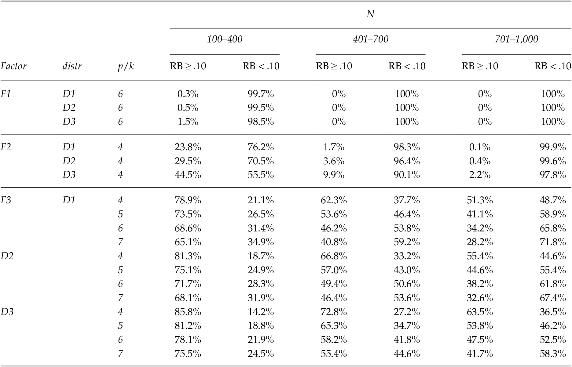
Table 1 presents the distribution, as percentages, of convergent and improper solutions gathered through CFA on the complete model, and on Factor 3 only, as a function of the simulated levels of p/k and N. Generally speaking, and in keeping with previous research results (e.g., Gagné & Hancock, Reference Gagné and Hancock2006), the highest percentage of improper solutions was observed when the complete model was analyzed under the least suitable conditions (e.g., 44.5% where p/k = 4 and N is between 100 and 200). The results improve as we raise p/k or N (23.9% where p/k = 7 and N is between 100 and 200; 19.2% where p/k = 4 and N is between 900 and 1,000). Under the most optimal conditions, the percentage of improper solutions drops below 5%. Likewise, the percentage of improper solutions found when CFA is applied to Factor 3 drops as p/k and N increase, falling below 1% when CFA on the complete model converges and the most optimal conditions are in place.
Table 1. Distribution of the Type of Solution Obtained Through Complete Model CFA vs. Factor 3 CFA

In the interest of simplicity, Table 1 does not include results from the simulated data distribution (distr: D1, D2, and D3). Please note, however, that the percentage of improper solutions observed when the complete model is analyzed increases in the asymmetric conditions, and that a compensatory effect is observed as a function of p/k and N (e.g., when p/k = 4 and N is between 100 and 200, a 40.1% rate of improper solutions is found in the symmetric condition (D1), 50.9% in the most asymmetric condition (D3); while for p/k = 6 and N between 501 and 600 produces rates of 8% and 14.7%, respectively). On the other hand, the number of UCV solutions also increases when the distribution is more asymmetric.
Overall, we found a rate of 17.4% improper solutions when applying CFA to the complete model, and just 11.5% when applying CFA to Factor 3 only. When the complete model is a convergent solution, and admissible, we also found a rate of 92.7% convergent solutions when Factor 3 was isolated. To summarize the above, using the strategy of isolating Factor 3 allowed us to differentiate between different assessment scenarios. On the one hand, finding an inadequate solution upon analyzing Factor 3 could be considered evidence against including it in the complete model, for lack of empirical consistency. Conversely, when the solution is convergent and admissible for the complete model as well as Factor 3, the χ ind 2 test helps determine if the isolated factor is an ACV solution or UCV solution. If the variance is acceptable, then it is best to proceed with evaluating the factor, while unacceptable variance would be further evidence not to include it in the model.
Table 1 illustrates that the percentage of UCV solutions is rather high given the magnitude of simulated λ ik for Factor 3, though it decreases as p/k and N increase. Results indicate that the percentage of UCV solutions is higher when the complete model yields improper solutions, which would explain (at least in part) why there was a lack of convergence in a model with various factors and various moderate to high factor loadings (Factors 1 and 2).
Stability Estimation and Rule-based Decision Making
We analyzed the degree to which λ ik* values for Factor 3 sufficiently capture the simulated values, using RB < 0.10 as the criterion to consider parameter recovery as acceptable (Forero et al., Reference Forero, Maydeu-Olivares and Gallardo-Pujol2009). That information was initially gathered by removing improper solutions produced by applying CFA to the complete model, and to Factor 3 on its own. Figure 2 presents the distribution of average λ ik* collected for Factor 3 by analyzing the complete model, taking into account p/k, N, and for the type of solution identified in the isolated Factor 3 CFA (bias: RB ≥ 0.10 and RB < 0.10; independence model: ACV and UCV solutions).
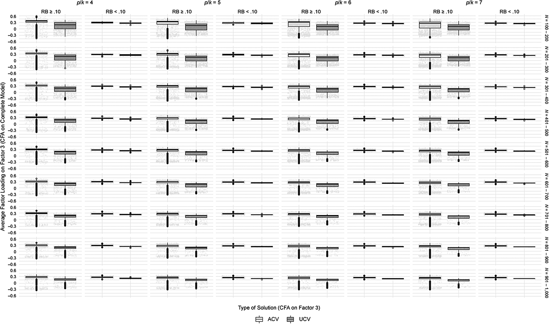
Figure 2. Factor 3 Average λik* from Complete Model CFA as a Function of p/k and N; Bias (RB); and Type of Solution (ACV or UCV).
Relative Bias < 0.10
The solutions where RB < 0.10 have average estimated factor loadings very close to the simulated averages (and very similar if one compares ACV to UCV solutions; see Figure 2). For the complete model, we recorded 36.2% of solutions with RB indices under 0.10. That level of precision improves as a function of p/k and N. For instance, there was a rate of 46.8% of this type of solution where p/k = 7, and 54.7% where N is between 900 and 1,000. We also found estimation was more accurate when the data were symmetrical (the percentages obtained combining p/k, N, and type of distribution appear in Table A.1 of Appendix A). Therefore, CFA has limited capacity for accurate parameter estimation in Factor 3, even in cases with an adequate number of items per factor, and observations. Under the circumstances, applying CFA to Factor 3 yields solutions with good estimation but unacceptable variance, which constitutes new evidence that the factor should not be included in the model.
Relative Bias ≥ 0.10
Figure 2 illustrates that average estimated λ ik* values for Factor 3 are higher when analyzing the complete model if there is acceptable variance in the solution identified through analyzing the isolated factor. In fact, these average values often exceed 0.3, although the simulated average was 0.25 (SD < 0.025), implying that RB ≥ 0.10. Thus, there is an overestimation issue for solutions in which a convergent and admissible solution is obtained by conducting both CFAs, and we would reject the null hypothesis of the χ ind 2 test for the isolated factor. In this case, applying arbitrary rules – such as eliminating items with factor loadings below a certain cutoff – could lead to mistaken decisions about the factor’s essential substance.
Examples of Solutions with Overestimated Parameters in Factor 3
For illustrative purposes only, Table 2 presents λ ik* values of Factor 3 for some of the solutions obtained through complete model CFA, as a function of the result obtained through isolated-Factor 3 CFA. Various criteria were used to select the examples appearing in Table 2 (E1 to E28), and to calculate the percentage of solutions present in the results as a function of p/k and N (for simplicity’s sake, N is sorted into three groups: 100–400, 401–700, and 701–1,000). We set two criteria to select examples where isolated-Factor 3 CFA yields an improper or UCV solution: If there are two or more λ ik* values over 0.3 and one λ ik* over 0.6 (presence of more than one over 0.6 is uncommon). To illustrate the type of solutions obtained when the solution has acceptable variance, we added the criterion of two or more λ ik* values over 0.4. λ ik* values that meet those selection criteria are indicated in bold.
Table 2. Examples of Estimated Solutions for Factor 3 in the Complete Model as a Function of p/k and N, and as a Function of the Isolated-Factor 3 CFA Outcome

Note. a Two or more λ ik* values > 0.3. b Two or more λ ik* values > 0.4. c One λ ik* value > 0.6.
With regard to the criterion of “two or more λ ik* values over 0.3,” when CFA on Factor 3 produced an improper solution (examples E1, E8, E15, and E22), we observed that the other λ ik* values were nearly zero, resulting in an underestimated average λ ik in the complete model. This type of solution was not very prevalent, since the most common was finding all (or almost all) λ ik* values below 0.3 (many negative), with averages even more underestimated than in the examples cited. This type of solution occurs less frequently when sample size is larger (increasing slightly along with p/k since the criterion becomes easier to meet, but without impacting the extent of average λ ik underestimation). When the result of CFA on Factor 3 is a UCV solution (examples E3, E10, E17, and E24), a similar pattern is observed, but with average λ ik values less underestimated. The percentage of solutions that meet the criterion is higher, although there is the same tendency for that to decrease as N increases. When the result of CFA on Factor 3 is an ACV solution (examples E5, E12, E19, and E26), the percentage of solutions with two or more λ ik* values over 0.3 is much higher, and the average value of λ ik tends to be overestimated.
The criterion “two or more λ ik* values over 0.4” was evaluated only when CFA on Factor 3 produced an ACV solution. Overall, the incidence of this type of solution is situated above 25% in samples of 100–400, decreasing to under 5% in sample sizes higher of 700. These results are consistent with De Winter et al. (Reference de Winter, Dodou and Wieringa2009) findings. Those authors showed that under conditions where N and λ ik are not too high, high λ ik* values may be found spuriously as a result of high standard error. The examples laid out in Table 2 (E6, E13, E20, and E27) suggest clear overestimation of average λ ik, with two or more λ ik* values over 0.4 and another over 0.3. For instance, solution E20 presents two λ ik* values above 0.4 (λ143* = 0.429 and λ163* = 0.419), and another three between 0.3 and 0.4 (λ113* = 0.369, λ133* = 0.350, and λ153* = 0.324). In the event of this type of solution, our understanding is it is common practice to admit all items, but that decision would be doubly unjustified: first because it is taken heuristically (based on the result), and second because the research could lend substantiveness to a factor that is clearly overestimated.
Another interesting result, indicated in the examples compiled in Table 2, is that practically no solutions were found in which all or almost all λ ik* values were overestimated
above 0.4. That heterogeneity of λ ik* values may indicate that the evaluated factor is unstable and would be hard to replicate. If we refer to simulated Factors 1 and 2 from this study (see Table A.1 of Appendix A), adequate recovery is shown by the fact that no λ ik* values were dissonant with the rest (in other words, showing clear signs of under- or overestimation). Only in Factor 2 with asymmetric data and N between 100 and 400, the incidence of solutions with RB < 0.10 was below 75%.
Regarding the criterion “one λ ik* over 0.6,” Table 2 indicates a higher frequency when the CFA on Factor 3 yields an ACV solution (examples E7, E14, E21, and E28). Type of solution becomes less prevalent as p/k and N increase. Presented with a case like this, researchers would often decide to interpret items with such high λ ik* values as good indicators or even markers of a factor (Ferrando & Anguiano-Carrasco, Reference Ferrando and Anguiano-Carrasco2010). When CFA on Factor 3 produces an improper or UCV solution, the remaining λ ik* values are very close to zero, so it is not wise to judge the quality of a factor based on one item. However, in ACV solutions and ones with 6 or 7 items, the other λ ik* values are higher. Several might even surpass the 0.4 cutoff as in example E28, which might lead to incorrect decisions about the factor’s substantiveness.
Goodness of Fit Assessment
Generally speaking, the GoF indices analyzed in this study suggest adequate fit in the case of complete model CFA: p-value of χ2 (M = 0.768, SD = 0.255), RMSEA (M = 0.002, SD = 0.006), SRMR (M = 0.046, SD = 0.016), and CFI (M = 0.999, SD = 0.005). These results do not differ much from the isolated-Factor 3 CFA findings: p-value of χ2 (M = 0.576, SD = 0.276), RMSEA (M = 0.008, SD = 0.015), SRMR (M = 0.031, SD = 0.015), and CFI (M = 0.960, SD = 0.095). A slight effect of the number of items in each model is observed, such that SRMR is slightly lower when CFA is applied to Factor 3 (analyzing fewer items); and CFI is higher in cases of complete model CFA. CFI compares the value of χ2 in the evaluated model to the value of χ ind 2, such that higher χ ind 2 produces a higher result. As mentioned, χ ind 2 is clearly higher in the case of complete model CFA than isolated-Factor 3 CFA.
GoF performance declines upon examining the worst simulated conditions. Accordingly, where N is between 100 and 200, and the distribution is asymmetrical (D3)Footnote 1, complete model CFA produced the following results: p-value of χ2 (M = 0.588, SD = 0.314), RMSEA (M = 0.010, SD = 0.015), SRMR (M = 0.093, SD = 0.012), and CFI (M = 0.990, SD = 0.020). Conversely, CFA on Factor 3 produced these results: p-value of χ2 (M = 0.590, SD = 0.274), RMSEA (M = 0.014, SD = 0.025), SRMR (M = 0.060, SD = 0.022), y CFI (M = 0.938, SD = 0.137). These findings suggest that GoF indices may reflect poor fit in some cases (at least partially, particularly for SRMR for complete model CFA, and CFI for Factor–3 CFA). Nonetheless, the number of such solutions is not very high, and they occur under CFA conditions that are not really advisable. Thus, the analyzed GoF (among the most widely used) do not seem useful at detecting factors with poor common variance, like the ones simulated in this study (Factor 3). These results are consistent with previous findings (Heene et al., Reference Heene, Hilbert, Draxler, Ziegler and Bühner2011). On another note, GoF indices for Factor–3 CFA do not allow for identification of the parameter overestimation issue discussed above (RB ≥ 0.10). Instead its GoF indices showed generally good fit in the case of ACV and UCV solutions, with UCV performing slightly better (see Appendix B).
Discussion
The applied researcher needs a solid theoretical and empirical foundation to make substantive interpretations of factor models based on specific samples, and to use instruments, scales, or tests scores with certain evidence of their validity. Furthermore, to guarantee an adequate parameter estimation process, the researcher must have access to large samples, the content of the factors should be well represented, and items should have ample measurement quality and show a clear relationship to the factors under evaluation. The problem is that many applications of CFA are conducted with suboptimal conditions and shaky decision making. In such situations, CFA lacks the empirical and substantive consistency desired for scientific measurement (Bollen, Reference Bollen1989), at least in a few sections or parts the evaluated model attempts to capture (e.g., a particular factor). That may have meaningful repercussions on the validity of the measurements.
In our judgment, the proliferation of recommendations about λ ik* values, paired with certain norms and reporting practices have contributed to what has become a generalized use of arbitrary cutoffs, without due regard for the consequences. The results of the present study reflect the compensatory nature of N, p/k, and λ ik, in keeping with previous findings (e.g., Gagné & Hancock, Reference Gagné and Hancock2006; Heene et al., Reference Heene, Hilbert, Draxler, Ziegler and Bühner2011). Those variables’ capacity to compensate for one another has a direct impact on the outcomes of parameter estimation, suggesting that decisions should not be based on any specific value. Please note that λ ik showed itself to be the most influential variable under these simulated conditions, requiring the strongest conditions of N and p/k to clearly show a compensatory effect on parameter estimation when λ ik magnitudes are low. That is shown by the average estimated factor loadings of each Factor 3 solution, and most especially by the estimated factor loading of each item.
One of the main limitations confronting the applied researcher is that they have no grounds on which to compare estimated factor loadings, because the magnitudes of population parameters are unknown. The results of the present study indicate that the analyzed conditions for CFA produce solutions with too much uncertainty. Therefore, rather than propose what minimum conditions ought to be met to conduct CFA, our recommendation is to apply that technique under conditions that guarantee appropriate estimation of factor loadings. Like Brown (Reference Brown2015), from here we encourage researchers – instead of applying a series of inflexible rules – to conduct their own simulations based on previously collected data, identify the optimal set of conditions suited to their particular applied context, and maybe tackle questions not addressed in the present study (non-normal and missing data, analysis of dichotomous items, etc.). For example, if the available sample size is questionable, Brown (Reference Brown2015) suggests conducting a Monte Carlo study using estimated parameters as population parameters to verify the statistical power and stability of parameter recovery. If a researcher aims to replicate and reanalyze models originating in other studies, they could use earlier results such as population parameters as a basis for simulation, and study the impact of different issues or limitations relating to the new applied conditions. The presumed stability of parameter estimation should be clearly reported in the results of any such simulation study. Moreover, simulation results can be shared with the research community in order to expand their potential replicability. Ondé and Alvarado (Reference Ondé and Alvarado2018) offer a detailed guide on how to conduct simulation studies using a CFA framework, and how to report the results thereof.
Precise estimation is the first step in the process of substantively interpreting a factor model solution. Once that is established, one should consider the practical significance of each factor according to the test’s end use, content validity, and capacity to predict other variables or constructs.
This study assesses a strategy proposed by Jöreskog and Sörbom (Reference Jöreskog and Sörbom1993): Isolate factors with CFA as a prerequisite step before evaluating the entire multi-factor model. Isolating factors allowed us to identify which simulated conditions lead to a high percentage of improper solutions that are not detected when evaluating the complete model. Moreover, by isolating factors we were able to identify factors with no significant common variance, solutions that are also not detected when evaluating the complete model. This strategy brought to the fore two interesting questions, one relating to applied research and one to simulation studies. Regarding the first, a stable solution should be largely replicable when parameters are estimated through isolated-Factor CFA. Regarding the second, a simulation study to evaluate the recovery of low factor loadings on a particular factor may cause bias in the results if it fails to differentiate between ACV and UCV solutions. That is because on average, UCV solutions are overestimated less. Additionally, testing the independence model on isolated factors can help to overcome the limitations of individual statistical tests of each parameter (Brown, Reference Brown2015; Mulaik, Reference Mulaik2009). That said, this question requires additional research.
The present study describes – through 28 examples - situations that applied researchers may encounter when conducting CFA, in which decisions are not reached merely by looking at λ ik* values and applying a golden rule or relying on goodness of fit measures. Many of these scenarios were plagued by clear overestimation of multiple parameters, leading to solutions appearing to be adequate. Some critical scenarios were identified: (a) Factor solutions with no common variance – statistically speaking – with factor loadings > 0.3; (b) solutions in which some items are severely overestimated, and therefore may be interpreted as good indicators or even markers of the factor; (c) solutions with poor common variance, where eliminating one item could lead to meaningfully underrepresenting the content of the factor; (d) clearly overestimated solutions in which the researcher might be tempted to apply the rule of 0.3 as a heuristic strategy, in an effort to avoid underrepresenting the content of the factor; and (e) solutions with good parameter recovery, but limited common variance. The overestimation problem is more worrisome when estimated factor loadings above 0.4 are obtained since it could be incorrectly assumed that they are more indicative of the item-factor relationship. These results have direct implications for applied research: in situations where the researcher doubts the stability of factor loadings estimation for a given factor; or replicates the study in new samples under more favorable conditions (the results suggest a need for at least five items per factor, and samples no smaller than 500 observations); or carries out a simulation to try and gather evidence of stability. We believe, too, that the present findings extend to the work of reviewing articles in the publication process.
We believe the examples presented here illustrate a variety of applied situations. Therefore, it is relatively common to find important underestimations of certain factor loadings when CFA is conducted to validate an exploratory model applied to data from a pilot study. When EFA is first conducted, it is common to discard some items presenting low λ ik* values, a situation that may lead to a change in the internal structure of the model when CFA is conducted later. It might also be interesting to evaluate if there are factors that are theoretically irrelevant – “minor factors” – as a result of systematic error like method effects, how the items are written, or to acquiescence, among other reasons. These factors often take the form of one of the examples explored here; thus, it is important not to purge them from the model right away, so that one can ascertain and report its effect on measurement. Another situation illustrated by some of these examples, that should be the object of future research, is related to facets evaluation in a bifactor model. Facets are specific factors within the model that do not correlate with each other, but which often show a limited amount of common variance because part of the variability of each item is explained by the overall factor. Broadly, all these applied situations highlight the importance of justifying any decision to keep or eliminate items in a model.
Finally, in terms of research limitations, the simulation study presented in this paper was carried out based on one of many scenarios that may be tested. Additional investigation with new research conditions is warranted to allow for generalization of the isolated-factor strategy proposed in this work. Consider, for instance, simulating structures with different number of latent variables, using discrete items with less than five response options, collinearity, missing data, outliers, etc. The present study simulated factor structures with no correlation among factors. It is reasonable to expect that results may differ for multidimensional structures with some degree of correlation between factors, which is common in applied contexts (for example, Forero et al. (Reference Forero, Maydeu-Olivares and Gallardo-Pujol2009) reported higher rates of convergent solutions and more stable parameter estimation when factors were correlated). This question too requires further research. We believe another important step is to analyze the type of decisions that get made when conditions are such that some items have common variance with more than one factor (cross-loading or double-loading), a frequent occurrence in applied contexts. On another note, the simulated data distribution produced interesting results (one symmetrical and two negatively skewed), but this variable was not evaluated in great depth. First, because simulating different types of distribution effectively bolsters the generalizability of results; and second, because it is more consistent with the literature reviewed (with greater emphasis on evaluating the effect of λ ik, p/k, and N). It is worth noting that data distribution in applied contexts often presents different degrees of skewness, so it would be prudent to explore any effect of heterogeneous distribution types (that is, different proportions of items with positive and negative skewness) on parameter recovery to improve the generalizability of results. In any case, the present work has shown that researchers can conduct simulation studies to determine the scope of their results, as an alternative to repeating the study in new samples.
Appendix A
Factor 3 Parameter Estimation Bias (Complete Model CFA)
Table A.1 Parameter Estimation for the Complete Model as a Function of p/k, N, and distr
Note. % Row of solutions where RB ≥ 0.10 and RB < 0.10.
Appendix B:
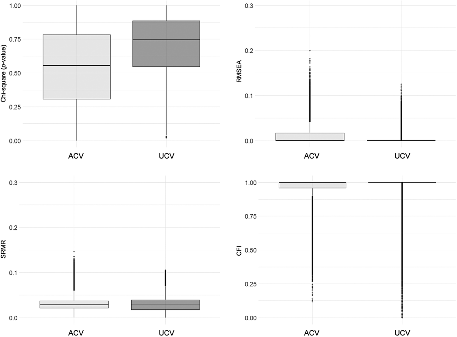
Figure B.1 Factor 3 Goodness of Fit, Comparing Solutions with Acceptable vs. Unacceptable Variance Note. Distribution of χ2 p-value, RMSEA, SRMR, and CFI as a function of the type of solution obtained through CFA on Factor 3 (ACV and UCV).


