


1 Introduction
Convection in the Earth’s mantle is largely driven by internal energy sources, involving heat released by the radioactive decay of long-lived isotopes of uranium, thorium and potassium and sensible heat extracted through secular cooling (Schubert, Turcotte & Olson Reference Schubert, Turcotte and Olson2001; Jaupart et al.
Reference Jaupart, Labrosse, Lucazeau and Mareschal2015). The Earth’s mantle is also heated from below by the Earth’s core but the magnitude of the basal heat flux is not known precisely. Today’s mantle motions are organized in two radically different planforms and spatial scales. The dominant planform is a set of thin subduction zones stretching over large distances at the edges of oceanic plates, where cold lithosphere goes down. These downwellings are associated with positive seismic velocity anomalies that can be traced to great depths (van der Hilst & Kárason Reference van der Hilst and Kárason1999). The return flow proceeds through mid-ocean ridges, but these are not underlain by deep-seated seismic anomalies, indicating that flow is essentially of a passive nature (Ritsema et al.
Reference Ritsema, Deuss, Van Heijst and Woodhouse2011). These are hallmarks of convection in an internally heated system that is cooled from above, where motions are driven by density variations generated in an unstable thermal boundary layer at the top (Roberts Reference Roberts1967; Kulacki & Goldstein Reference Kulacki and Goldstein1972; Parmentier, Sotin & Travis Reference Parmentier, Sotin and Travis1994; Goluskin Reference Goluskin2016; Vilella et al.
Reference Vilella, Limare, Jaupart, Farnetani, Fourel and Kaminski2018). In the Earth, convection also involves a number of narrow upwellings feeding intraplate volcanoes called ‘hotspots’, such as beneath Hawaii and Reunion islands. Many prominent hotspots stand above nearly vertical negative seismic velocity anomalies that extend down to the top of the core (Montelli et al.
Reference Montelli, Nolet, Dahlen and Masters2006; French & Romanowicz Reference French and Romanowicz2015). These observations appear to support the traditional mantle plume model that calls for basal heating by the Earth’s core. These plumes are not distributed at random, however, and are linked to large anomalous structures in the lowermost mantle. High-resolution seismic studies have revealed that the
 ${\approx}$
200–300 km thick so-called D
${\approx}$
200–300 km thick so-called D
 $^{\prime \prime }$
basal layer is in fact not laterally continuous. It is more appropriate to refer to a basal region of several hundred kilometres thickness where material is anomalous and much more heterogeneous than the rest of the lower mantle (Garnero & Helmberger Reference Garnero and Helmberger1996; Garnero, McNamara & Shim Reference Garnero, McNamara and Shim2016). Seismic wave speeds are anomalously low in two broad regions called large low-shear-velocity provinces (LLSVPs), which extend over a thickness of as much as 1000 km above the core–mantle boundary and which are difficult to reconcile with convection in a homogeneous mantle. Of particular interest is that hotspot seismic anomalies preferentially lie at the edges of these LLSVPs (Torsvik et al.
Reference Torsvik, Smethurst, Burke and Steinberger2006; Deschamps, Cobden & Tackley Reference Deschamps, Cobden and Tackley2012; Garnero et al.
Reference Garnero, McNamara and Shim2016; Li et al.
Reference Li, McNamara, Garnero and Yu2017).
$^{\prime \prime }$
basal layer is in fact not laterally continuous. It is more appropriate to refer to a basal region of several hundred kilometres thickness where material is anomalous and much more heterogeneous than the rest of the lower mantle (Garnero & Helmberger Reference Garnero and Helmberger1996; Garnero, McNamara & Shim Reference Garnero, McNamara and Shim2016). Seismic wave speeds are anomalously low in two broad regions called large low-shear-velocity provinces (LLSVPs), which extend over a thickness of as much as 1000 km above the core–mantle boundary and which are difficult to reconcile with convection in a homogeneous mantle. Of particular interest is that hotspot seismic anomalies preferentially lie at the edges of these LLSVPs (Torsvik et al.
Reference Torsvik, Smethurst, Burke and Steinberger2006; Deschamps, Cobden & Tackley Reference Deschamps, Cobden and Tackley2012; Garnero et al.
Reference Garnero, McNamara and Shim2016; Li et al.
Reference Li, McNamara, Garnero and Yu2017).
Geochemical data confirm that the Earth’s mantle is heterogeneous and indicate the presence of different materials, primordial mantle, mantle that has been depleted through melting and possibly a second type of primordial mantle inherited from early planetary formation and differentiation processes (Hofmann Reference Hofmann2003; Gale et al. Reference Gale, Dalton, Langmuir, Su and Schilling2013). These contain different amounts of radioactive elements, implying that heat sources are not uniformly distributed (Turcotte, Paul & White Reference Turcotte, Paul and White2001; Javoy & Kaminski Reference Javoy and Kaminski2014). One type of material is the consequence of melt extraction at shallow depths beneath ocean ridges and trenches, which generates a depleted oceanic lithosphere and enriched continental crust, processes which have been active over most of Earth’s history. A second type may be inherited from early planetary processes (Javoy & Kaminski Reference Javoy and Kaminski2014) and may have survived for several billions of years. How it was generated remains unclear. Contributing mechanisms include the settling of iron phases and crystallization in an early magma ocean phase. Iron-silicate and melt-solid equilibria depend on pressure, implying that the primordial mantle composition was likely to depend on depth. The locations of the different mantle materials remain debated. What is known with certainty is that continental crust has been extracted from the mantle, leaving a residue that has been qualified as ‘depleted’. Because continental crust is a concentrate of heat-producing elements, ‘depletion’ adequately reflects the impact of crust formation on the mantle with respect to internal heating (Turcotte et al. Reference Turcotte, Paul and White2001). The upper mantle is made of different materials mixed in variable proportions, including primordial mantle brought by deep plumes (Gale et al. Reference Gale, Dalton, Langmuir, Su and Schilling2013). Mass balance constraints are met with a three reservoir structure, made of a primordial basal region, a depleted mid-mantle and an only slightly depleted upper mantle (Jackson & Carlson Reference Jackson and Carlson2012; Gale et al. Reference Gale, Dalton, Langmuir, Su and Schilling2013). The difference between the upper and mid-mantle reservoirs is due to subduction, which goes through the former and continuously injects newly depleted material into the latter.
The presence of undepleted primordial material with higher than average heat production at the bottom of the mantle makes for a deep supply of heat able to generate upwelling activity. Thus, mantle plumes may be due to heat coming from the core as well as heat produced in a basal reservoir. Discriminating between these two contributions is important because they involve different physical controls and are not likely to follow the same time evolution. There is little doubt that the Earth’s core cannot host significant amounts of radioactive elements, implying that it can only heat the mantle if it is cooling down. The heat flux out of the core depends on thermal coupling with the highly viscous mantle, and has probably changed with time. In an initially thermally well-mixed planet, for example, this heat flux would have been zero. In similar fashion, the amount of primordial material at the base of the mantle cannot be taken as constant because convective motions are bound to induce mixing with the overlying material.
Starting from two layers of different materials, mixing may proceed by two different processes, the folding of one fluid over the other and the tearing out of thin schlieren at the interface (Olson & Kincaid Reference Olson and Kincaid1991). The latter process operates at very small scales and presents a difficult challenge for direct numerical simulations (Deschamps & Tackley Reference Deschamps and Tackley2008, Reference Deschamps and Tackley2009). Quantitative laboratory studies have been carried out in Rayleigh–Bénard set-ups with fixed temperatures at the top and bottom or a fixed heat flux (Richter & McKenzie Reference Richter and McKenzie1981; Olson Reference Olson1984; Olson & Kincaid Reference Olson and Kincaid1991; Davaille Reference Davaille1999a ,Reference Davaille b ). These experiments reveal a wealth of phenomena such as the oscillatory motions of plumes initiated in a dense lower layer and the overturn of the layers. They also show that protrusions of the lower layer into the upper one act to anchor upwellings at the same locations for long time intervals, with important implications for mantle convection (Davaille, Girard & Le Bars Reference Davaille, Girard and Le Bars2002; Jellinek & Manga Reference Jellinek and Manga2002). A recent study by Lepot, Aumaître & Gallet (Reference Lepot, Aumaître and Gallet2018) sheds light on heat transport in a fluid layer where internal heat sources are concentrated in a basal region. To the best of our knowledge, however, no experiments are available for internally heated compositionally stratified reservoirs, which leaves an important gap in studies of mantle convection.
In the Earth’s mantle, the distribution of heat sources affects the pattern and amplitude of convective motions and in turn gets modified by the flow. As explained above, one cannot consider that either the heat flux or temperature at the core–mantle boundary have remained constant through time. It is thus worthwhile to focus on a stand alone system powered by its heat sources with no heat supplied by a separate system. In order to study mixing phenomena over long time intervals quantitatively, we rely on laboratory experiments. We investigate the behaviour of a stratified reservoir that is cooled from above and that has a larger concentration of heat sources in a lower layer above an adiabatic boundary. Due to mixing, the internal structure becomes increasingly removed from the starting one. We track the time-dependent spatial pattern and temperature differences that drive convection and investigate how they depend on the control variables. In the Earth’s mantle, complete mixing, such that discriminating between individual material components is no longer possible at the smallest scale of relevance, involves solid-state diffusion and is unlikely due to the very small values of the diffusion coefficient, as indicated by geochemical data (Hofmann Reference Hofmann2003; Gale et al. Reference Gale, Dalton, Langmuir, Su and Schilling2013). We determine the time for the pervasive mingling of the two fluids, such that the initial two-layer configuration has been eradicated completely, and work out how and when the reservoir starts behaving as a homogeneous one.
The paper is organized as follows. We describe the experimental set-up and protocol as well as the relevant control variables and dimensionless numbers. We determine the bulk thermal evolution and surface heat flux and show that, after a small lead time, both depend weakly on the distribution of internal heat sources. We identify and characterize two convection regimes based on the statistical distribution of the interface depth. These two regimes depend on a buoyancy number which scales density differences due to temperature to the intrinsic density contrast between the two fluids and on the intensity of convective motions as measured by a Rayleigh number. We describe in detail the changes of thermal structure that are induced by mixing and derive empirical scaling laws for the temperature excess and the lifetime of the enriched lower layer. We discuss some implications of our results for the Earth’s mantle in a final section.
2 Dynamical regimes and governing parameters
2.1 Dimensionless numbers for homogeneous internally heated convection
In a homogeneous internally heated fluid layer that is cooled from above and that has an adiabatic base, the relevant temperature scale is:
 $$\begin{eqnarray}\displaystyle \unicode[STIX]{x0394}T_{H}={\displaystyle \frac{Hh^{2}}{\unicode[STIX]{x1D706}}}, & & \displaystyle\end{eqnarray}$$
where
 $h$
is the reservoir thickness,
$h$
is the reservoir thickness,
 $\unicode[STIX]{x1D706}$
is thermal conductivity and
$\unicode[STIX]{x1D706}$
is thermal conductivity and
 $H$
is the rate of heat generation per unit volume. Using standard scales for time, velocity and length, the governing Boussinesq equations lead to two dimensionless numbers, the Rayleigh–Roberts number
$H$
is the rate of heat generation per unit volume. Using standard scales for time, velocity and length, the governing Boussinesq equations lead to two dimensionless numbers, the Rayleigh–Roberts number
 $Ra_{H}$
and the Prandtl number
$Ra_{H}$
and the Prandtl number
 $Pr$
(Roberts Reference Roberts1967):
$Pr$
(Roberts Reference Roberts1967):
 $$\begin{eqnarray}\displaystyle Ra_{H}={\displaystyle \frac{\unicode[STIX]{x1D70C}g\unicode[STIX]{x1D6FC}Hh^{5}}{\unicode[STIX]{x1D706}\unicode[STIX]{x1D705}\unicode[STIX]{x1D707}}}, & & \displaystyle\end{eqnarray}$$
and
 $$\begin{eqnarray}\displaystyle Pr={\displaystyle \frac{\unicode[STIX]{x1D708}}{\unicode[STIX]{x1D705}}}, & & \displaystyle\end{eqnarray}$$
where
 $\unicode[STIX]{x1D70C}$
is the density at some reference temperature,
$\unicode[STIX]{x1D70C}$
is the density at some reference temperature,
 $g$
is the acceleration of gravity,
$g$
is the acceleration of gravity,
 $\unicode[STIX]{x1D6FC}$
is the thermal expansion coefficient,
$\unicode[STIX]{x1D6FC}$
is the thermal expansion coefficient,
 $\unicode[STIX]{x1D705}$
is the thermal diffusivity,
$\unicode[STIX]{x1D705}$
is the thermal diffusivity,
 $\unicode[STIX]{x1D707}$
is the dynamic viscosity and
$\unicode[STIX]{x1D707}$
is the dynamic viscosity and
 $\unicode[STIX]{x1D708}=\unicode[STIX]{x1D707}/\unicode[STIX]{x1D70C}$
is the kinematic viscosity. For sufficiently large values of
$\unicode[STIX]{x1D708}=\unicode[STIX]{x1D707}/\unicode[STIX]{x1D70C}$
is the kinematic viscosity. For sufficiently large values of
 $Pr$
, inertial effects are negligible compared to viscous effects and one can work in the infinite Prandtl limit. In these conditions, which are certainly those of telluric planets with
$Pr$
, inertial effects are negligible compared to viscous effects and one can work in the infinite Prandtl limit. In these conditions, which are certainly those of telluric planets with
 $Pr>10^{23}$
, the characteristics of convection depend only on
$Pr>10^{23}$
, the characteristics of convection depend only on
 $Ra_{H}$
.
$Ra_{H}$
.
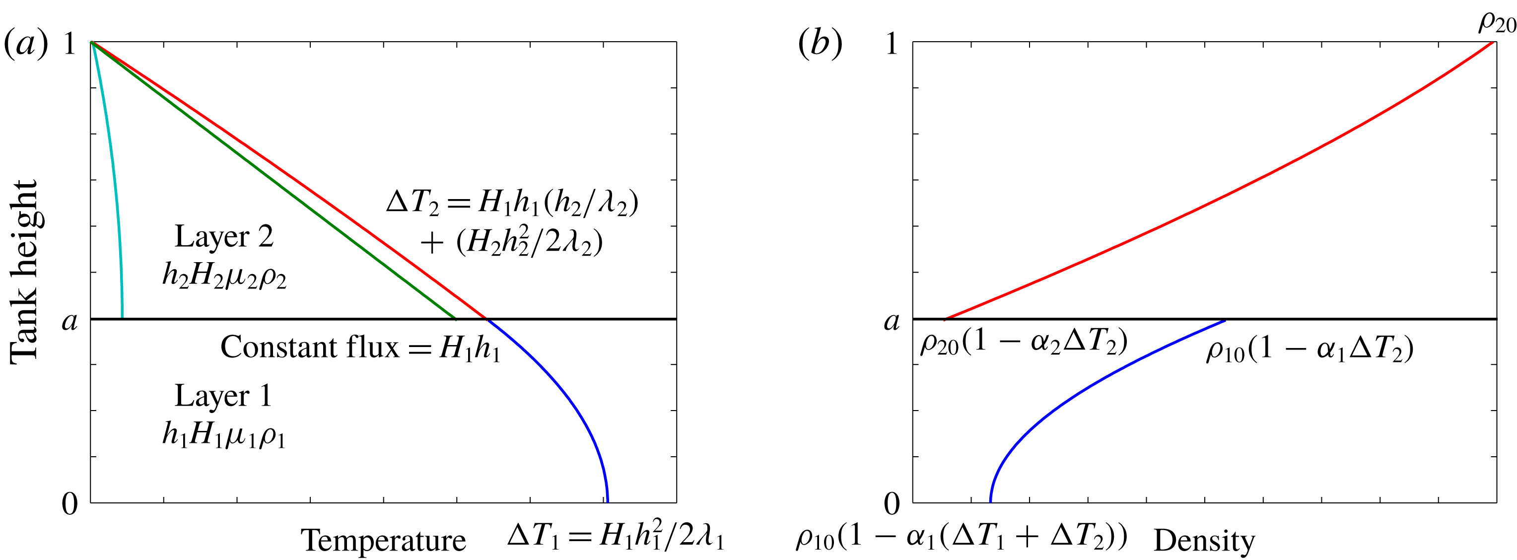
Figure 1. Conduction temperature profile (a) and the corresponding density profile (b) in a two-layer reservoir. (a) Temperature elevation in layer 2 due to internal heating only (light blue), temperature elevation in layer 2 due to the heat flux at its base (green), total temperature profile in layer 2 (red) and temperature profile in layer 1 due to internal heating only (blue). (b) Density profile in layer 2 (red) and in layer 1 (blue).
2.2 Dimensionless numbers for a two-layer system
We investigate convection in an initially two-layer reservoir involving two miscible fluids with different physical properties and thicknesses (figure 1). The upper surface is kept at a constant temperature and the lower one is adiabatic. The two fluids have identical coefficients of thermal expansion, thermal conductivities and heat capacities, as in the Earth’s mantle, where the small variations of composition that exist have no significant impact on these properties. In contrast, viscosity values and rates of internal heat generation in mantle material are very sensitive to trace amounts of water and radioactive elements, respectively. The rheological properties of mantle rocks also depend on pressure, stress, grain size and mineral composition, but these effects will be ignored here for simplicity. We therefore consider two fluids which differ by their intrinsic densities, viscosities and heat generation rates. Our working fluids are dilute aqueous solutions of sodium chloride salt and hydroxyethylcellulose, a compound that induces large viscosity changes for very small concentrations.
In the following, indices 1 and 2 will refer to the lower and upper layers, respectively. Equations of state are as follows:
 $$\begin{eqnarray}\displaystyle \unicode[STIX]{x1D70C}_{i}=\unicode[STIX]{x1D70C}_{io}[1-\unicode[STIX]{x1D6FC}(T-T_{o})], & & \displaystyle\end{eqnarray}$$
where
 $i=1,2$
refers to each fluid. Reference temperature
$i=1,2$
refers to each fluid. Reference temperature
 $T_{o}$
is that of the upper surface and can be taken as equal to zero. The two fluids occupy a total thickness
$T_{o}$
is that of the upper surface and can be taken as equal to zero. The two fluids occupy a total thickness
 $h$
initially split into two layers with thicknesses
$h$
initially split into two layers with thicknesses
 $h_{1}$
and
$h_{1}$
and
 $h_{2}$
, such that
$h_{2}$
, such that
 $h=h_{1}+h_{2}$
. Thickness ratio
$h=h_{1}+h_{2}$
. Thickness ratio
 $a=h_{1}/h$
is equal to the volume fraction of the lower fluid and remains a key control variable even when the layered structure has been destroyed. With heat production rates
$a=h_{1}/h$
is equal to the volume fraction of the lower fluid and remains a key control variable even when the layered structure has been destroyed. With heat production rates
 $H_{1}$
and
$H_{1}$
and
 $H_{2}$
in the lower and upper fluids, respectively, the total rate of heat released in the reservoir is:
$H_{2}$
in the lower and upper fluids, respectively, the total rate of heat released in the reservoir is:
 $$\begin{eqnarray}\displaystyle Hh=H_{1}h_{1}+H_{2}h_{2}. & & \displaystyle\end{eqnarray}$$
We define an enrichment factor for the lower fluid as follows:
 $$\begin{eqnarray}\displaystyle F={\displaystyle \frac{H_{1}}{H}}, & & \displaystyle\end{eqnarray}$$
and a viscosity ratio:
 $$\begin{eqnarray}\displaystyle \unicode[STIX]{x1D6FE}={\displaystyle \frac{\unicode[STIX]{x1D707}_{1}}{\unicode[STIX]{x1D707}_{2}}}. & & \displaystyle\end{eqnarray}$$
One last dimensionless number is needed to characterize the two-layer system, which is the buoyancy number (i.e. the ratio of the stabilizing density anomaly to the destabilizing thermal anomaly):
 $$\begin{eqnarray}\displaystyle B={\displaystyle \frac{\unicode[STIX]{x1D70C}_{10}-\unicode[STIX]{x1D70C}_{20}}{\unicode[STIX]{x1D70C}\unicode[STIX]{x1D6FC}\unicode[STIX]{x0394}T}}={\displaystyle \frac{\unicode[STIX]{x0394}\unicode[STIX]{x1D70C}}{\unicode[STIX]{x1D70C}\unicode[STIX]{x1D6FC}\unicode[STIX]{x0394}T}}, & & \displaystyle\end{eqnarray}$$
where
 $\unicode[STIX]{x1D70C}_{10}-\unicode[STIX]{x1D70C}_{20}=\unicode[STIX]{x0394}\unicode[STIX]{x1D70C}$
is the intrinsic density difference, that is the density difference due to composition only, as opposed to the actual density difference which depends on composition and temperature, and
$\unicode[STIX]{x1D70C}_{10}-\unicode[STIX]{x1D70C}_{20}=\unicode[STIX]{x0394}\unicode[STIX]{x1D70C}$
is the intrinsic density difference, that is the density difference due to composition only, as opposed to the actual density difference which depends on composition and temperature, and
 $\unicode[STIX]{x0394}T$
is an appropriate scale for the temperature contrast between the two fluids. In a major difference with Rayleigh–Bénard experiments, this temperature contrast is not fixed and changes with time as mixing progresses. Temperature scales for the two layers can be determined using a conduction equilibrium reference state (figure 1
a). The appropriate boundary conditions are zero heat flux at the reservoir base (at
$\unicode[STIX]{x0394}T$
is an appropriate scale for the temperature contrast between the two fluids. In a major difference with Rayleigh–Bénard experiments, this temperature contrast is not fixed and changes with time as mixing progresses. Temperature scales for the two layers can be determined using a conduction equilibrium reference state (figure 1
a). The appropriate boundary conditions are zero heat flux at the reservoir base (at
 $z=0$
) and zero temperature at the top (at
$z=0$
) and zero temperature at the top (at
 $z=h$
). Integrating the diffusion heat equation and applying the continuity of temperature and heat flux at the interface (at
$z=h$
). Integrating the diffusion heat equation and applying the continuity of temperature and heat flux at the interface (at
 $z=h_{1}$
), one obtains:
$z=h_{1}$
), one obtains:
 $$\begin{eqnarray}\displaystyle & \displaystyle \unicode[STIX]{x0394}T_{1}(z)=H_{1}h_{1}{\displaystyle \frac{h_{2}}{\unicode[STIX]{x1D706}}}+{\displaystyle \frac{H_{2}{h_{2}}^{2}}{2\unicode[STIX]{x1D706}}}+{\displaystyle \frac{H_{1}{h_{1}}^{2}}{2\unicode[STIX]{x1D706}}}\left(1-{\displaystyle \frac{z^{2}}{{h_{1}}^{2}}}\right), & \displaystyle\end{eqnarray}$$
 $$\begin{eqnarray}\displaystyle & \displaystyle \unicode[STIX]{x0394}T_{2}(z)=H_{1}h_{1}{\displaystyle \frac{h-z}{\unicode[STIX]{x1D706}}}+{\displaystyle \frac{H_{2}{h_{2}}^{2}}{2\unicode[STIX]{x1D706}}}\left(1-{\displaystyle \frac{(z-h_{1})^{2}}{{h_{2}}^{2}}}\right). & \displaystyle\end{eqnarray}$$
Figure 1(b) shows the corresponding density distribution. The temperature differences across the two layers are, respectively:
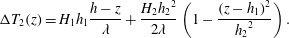
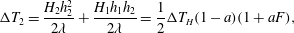 $$\begin{eqnarray}\displaystyle & \displaystyle \unicode[STIX]{x0394}T_{2}={\displaystyle \frac{H_{2}h_{2}^{2}}{2\unicode[STIX]{x1D706}}}+{\displaystyle \frac{H_{1}h_{1}h_{2}}{2\unicode[STIX]{x1D706}}}={\displaystyle \frac{1}{2}}\unicode[STIX]{x0394}T_{H}(1-a)(1+aF), & \displaystyle\end{eqnarray}$$
 $$\begin{eqnarray}\displaystyle & \displaystyle \unicode[STIX]{x0394}T_{1}={\displaystyle \frac{H_{1}h_{1}^{2}}{2\unicode[STIX]{x1D706}}}={\displaystyle \frac{1}{2}}\unicode[STIX]{x0394}T_{H}[1+a(F-1)], & \displaystyle\end{eqnarray}$$
where
 $\unicode[STIX]{x0394}T_{H}$
is the temperature scale for a homogeneous layer of thickness
$\unicode[STIX]{x0394}T_{H}$
is the temperature scale for a homogeneous layer of thickness
 $h$
and heat generation
$h$
and heat generation
 $H$
(2.1). The average temperature in each layer is obtained by integrating (2.9) and (2.10):
$H$
(2.1). The average temperature in each layer is obtained by integrating (2.9) and (2.10):
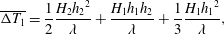 $$\begin{eqnarray}\displaystyle & \displaystyle \overline{\unicode[STIX]{x0394}T_{1}}={\displaystyle \frac{1}{2}}{\displaystyle \frac{H_{2}{h_{2}}^{2}}{\unicode[STIX]{x1D706}}}+{\displaystyle \frac{H_{1}h_{1}h_{2}}{\unicode[STIX]{x1D706}}}+{\displaystyle \frac{1}{3}}{\displaystyle \frac{H_{1}{h_{1}}^{2}}{\unicode[STIX]{x1D706}}}, & \displaystyle\end{eqnarray}$$
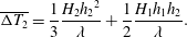 $$\begin{eqnarray}\displaystyle & \displaystyle \overline{\unicode[STIX]{x0394}T_{2}}={\displaystyle \frac{1}{3}}{\displaystyle \frac{H_{2}{h_{2}}^{2}}{\unicode[STIX]{x1D706}}}+{\displaystyle \frac{1}{2}}{\displaystyle \frac{H_{1}h_{1}h_{2}}{\unicode[STIX]{x1D706}}}. & \displaystyle\end{eqnarray}$$
The global temperature difference between the two layers is thus:
 $$\begin{eqnarray}\displaystyle \unicode[STIX]{x0394}T=\overline{\unicode[STIX]{x0394}T_{1}}-\overline{\unicode[STIX]{x0394}T_{2}}={\textstyle \frac{1}{6}}\unicode[STIX]{x0394}T_{H}(1-a+2aF). & & \displaystyle\end{eqnarray}$$
This temperature difference corresponds to a reference thermal structure and illustrates the influence of several dimensionless numbers. It is likely to be very different from that of the fully convecting system, however, and we shall also consider an ‘effective’ temperature difference determined in the course of an experiment. In the following, we shall use two different temperature scales. To deal with the coupling between the two fluids, we use both the conduction thermal contrast
 $\unicode[STIX]{x0394}T$
(2.15) and the ‘effective’ temperature difference, and we shall show that the latter is related to the former. For the bulk evolution of the whole reservoir, it is more appropriate to use the bulk scale
$\unicode[STIX]{x0394}T$
(2.15) and the ‘effective’ temperature difference, and we shall show that the latter is related to the former. For the bulk evolution of the whole reservoir, it is more appropriate to use the bulk scale
 $\unicode[STIX]{x0394}T_{H}$
.
$\unicode[STIX]{x0394}T_{H}$
.
Convection in the lower layer is driven by internal heat sources only, and hence can be characterized by its local Rayleigh–Roberts number
 $Ra_{H1}$
:
$Ra_{H1}$
:
 $$\begin{eqnarray}\displaystyle Ra_{H1}={\displaystyle \frac{\unicode[STIX]{x1D70C}_{1o}g\unicode[STIX]{x1D6FC}H_{1}{h_{1}}^{5}}{\unicode[STIX]{x1D706}\unicode[STIX]{x1D705}\unicode[STIX]{x1D707}_{1}}}. & & \displaystyle\end{eqnarray}$$
In contrast, the upper layer is heated by both internal heat sources and by the lower fluid. Thus, convection depends not only on the Rayleigh–Roberts number
 $Ra_{H2}$
for the layer, defined as above with the relevant properties, but also on the relative importance of the two types of heat input. We introduce two dimensionless numbers. The first one, noted
$Ra_{H2}$
for the layer, defined as above with the relevant properties, but also on the relative importance of the two types of heat input. We introduce two dimensionless numbers. The first one, noted
 $Ra_{2}$
, relies on the total heat flux at the top of the upper fluid in steady-state conditions and can be written as a function of
$Ra_{2}$
, relies on the total heat flux at the top of the upper fluid in steady-state conditions and can be written as a function of
 $Ra_{H2}$
and a second dimensionless number noted
$Ra_{H2}$
and a second dimensionless number noted
 $E$
:
$E$
:
 $$\begin{eqnarray}\displaystyle Ra_{2}={\displaystyle \frac{\unicode[STIX]{x1D70C}_{2o}g\unicode[STIX]{x1D6FC}\left(H_{1}{\displaystyle \frac{h_{1}}{h_{2}}}+H_{2}\right){h_{2}}^{5}}{\unicode[STIX]{x1D706}\unicode[STIX]{x1D705}\unicode[STIX]{x1D707}_{2}}}=Ra_{H2}(E+1), & & \displaystyle\end{eqnarray}$$
where
 $E$
is the ratio between the two different contributions to the heat flux at the top of the reservoir.
$E$
is the ratio between the two different contributions to the heat flux at the top of the reservoir.
 $$\begin{eqnarray}\displaystyle E={\displaystyle \frac{H_{1}h_{1}}{H_{2}h_{2}}}. & & \displaystyle\end{eqnarray}$$
All the dimensionless numbers rely on the initial configuration of two layers separated by a horizontal interface, which may not be relevant in practice as the interface gets distorted and as the two fluids progressively mingle with one another. The viscosity of the final homogenized fluid can be estimated as follows (Bloomfield & Dewan Reference Bloomfield and Dewan1971):
 $$\begin{eqnarray}\displaystyle \unicode[STIX]{x1D707}={\unicode[STIX]{x1D707}_{1}}^{a}{\unicode[STIX]{x1D707}_{2}}^{1-a}. & & \displaystyle\end{eqnarray}$$
Using the bulk heat production for the reservoir,
 $H$
(2.5), this allows calculation of a ‘bulk’ Rayleigh–Roberts number for the homogenized reservoir, denoted by
$H$
(2.5), this allows calculation of a ‘bulk’ Rayleigh–Roberts number for the homogenized reservoir, denoted by
 $Ra_{H}$
as above.
$Ra_{H}$
as above.
It is useful to refer to the individual Rayleigh number for the two layers because it specifies their convection regimes in initial stages, but there are only five independent dimensionless numbers, which can be chosen to be
 $Ra_{H}$
,
$Ra_{H}$
,
 $\unicode[STIX]{x1D6FE}$
,
$\unicode[STIX]{x1D6FE}$
,
 $F$
,
$F$
,
 $a$
and
$a$
and
 $B$
, to which one should add
$B$
, to which one should add
 $Pr$
for completeness. All the other numbers can be derived from this list. For example:
$Pr$
for completeness. All the other numbers can be derived from this list. For example:
 $$\begin{eqnarray}\displaystyle E={\displaystyle \frac{aF}{1-aF}}. & & \displaystyle\end{eqnarray}$$
If
 $F=1$
, the lower layer has the same amount of heat sources as the upper one and the basal temperature is that of a homogeneous fluid layer,
$F=1$
, the lower layer has the same amount of heat sources as the upper one and the basal temperature is that of a homogeneous fluid layer,
 $(1/2)\unicode[STIX]{x0394}T_{H}$
. If
$(1/2)\unicode[STIX]{x0394}T_{H}$
. If
 $F=1/a$
, there are no heat sources in the upper layer and the bottom temperature is
$F=1/a$
, there are no heat sources in the upper layer and the bottom temperature is
 $\unicode[STIX]{x0394}T_{H}(1-a/2)$
, which is larger and illustrates the importance of heat sources at the base of the reservoir. Maintaining the constraint that
$\unicode[STIX]{x0394}T_{H}(1-a/2)$
, which is larger and illustrates the importance of heat sources at the base of the reservoir. Maintaining the constraint that
 $F=1/a$
, decreasing the value of
$F=1/a$
, decreasing the value of
 $a$
(
$a$
(
 $a\rightarrow 0$
) implies an increasing amount of heat sources in an increasingly thinner lower layer and produces a situation similar to Rayleigh–Bénard convection in the upper layer with a basal temperature set to
$a\rightarrow 0$
) implies an increasing amount of heat sources in an increasingly thinner lower layer and produces a situation similar to Rayleigh–Bénard convection in the upper layer with a basal temperature set to
 $\unicode[STIX]{x0394}T_{H}$
.
$\unicode[STIX]{x0394}T_{H}$
.
3 Laboratory set-up and experimental protocol
We rely on our new experimental set-up which was designed specifically to study convection due to internal heat sources. A complete description and discussion of measurement precision and accuracy may be found in Fourel et al. (Reference Fourel, Limare, Jaupart, Surducan, Farnetani, Kaminski, Neamtu and Surducan2017).
3.1 Experimental techniques
Working fluids were prepared in our laboratory in order to investigate a large range of dimensionless parameters. All were aqueous solutions of salt and hydroxyethylcellulose, which are fully miscible and whose intrinsic densities and viscosities can be varied within large ranges at small cost. Sodium chloride salt increases both density and microwave absorption. New fluids were used for each experiment and physical properties were determined over the relevant temperature range. Viscosity was measured to better than a few per cent uncertainty with a Thermo Scientific Haake rheometer RS600. Prandtl numbers were always larger than
 $10^{2}$
, which ensures the dominance of viscous stresses over inertia, as in the Earth’s mantle (Davaille & Limare Reference Davaille, Limare and Schubert2015). Over the typical temperature range of an experiment (
$10^{2}$
, which ensures the dominance of viscous stresses over inertia, as in the Earth’s mantle (Davaille & Limare Reference Davaille, Limare and Schubert2015). Over the typical temperature range of an experiment (
 $10\,^{\circ }\text{C}$
), viscosity varies by a factor of about 0.6. A careful comparison between high-precision numerical calculations with or without such variations shows that viscosity changes of this magnitude have no significant effect on the variables of interest and on scaling laws (Limare et al.
Reference Limare, Vilella, Di Giuseppe, Farnetani, Kaminski, Surducan, Surducan, Neamtu, Fourel and Jaupart2015). For density and thermal expansion coefficient, we used a DMA 5000 Anton Paar densimeter with an accuracy of one part per million. Thermal diffusivity and conductivity were determined by the photopyroelectric method (Dadarlat & Neamtu Reference Dadarlat and Neamtu2009), and dielectric properties with an Agilent N5230A vector network analyser. The salt diffusion coefficient in polymerized fluids such as ours was estimated for different polymer concentration and decreases with increasing polymer concentration (and hence with increasing fluid viscosity) (Davaille Reference Davaille1999b
). At the interface between two layers of different viscosities, chemical diffusion is limited by the fluid with the smallest diffusion coefficient (in the most viscous one). In this series of experiments, relevant values of the diffusion coefficient lie in a
$10\,^{\circ }\text{C}$
), viscosity varies by a factor of about 0.6. A careful comparison between high-precision numerical calculations with or without such variations shows that viscosity changes of this magnitude have no significant effect on the variables of interest and on scaling laws (Limare et al.
Reference Limare, Vilella, Di Giuseppe, Farnetani, Kaminski, Surducan, Surducan, Neamtu, Fourel and Jaupart2015). For density and thermal expansion coefficient, we used a DMA 5000 Anton Paar densimeter with an accuracy of one part per million. Thermal diffusivity and conductivity were determined by the photopyroelectric method (Dadarlat & Neamtu Reference Dadarlat and Neamtu2009), and dielectric properties with an Agilent N5230A vector network analyser. The salt diffusion coefficient in polymerized fluids such as ours was estimated for different polymer concentration and decreases with increasing polymer concentration (and hence with increasing fluid viscosity) (Davaille Reference Davaille1999b
). At the interface between two layers of different viscosities, chemical diffusion is limited by the fluid with the smallest diffusion coefficient (in the most viscous one). In this series of experiments, relevant values of the diffusion coefficient lie in a
 $10^{-12}$
–
$10^{-12}$
–
 $10^{-13}~\text{m}^{2}~\text{s}^{-1}$
range. For a reference time interval of 3 h (the typical duration of an experiment), these lead to diffusion lengths
$10^{-13}~\text{m}^{2}~\text{s}^{-1}$
range. For a reference time interval of 3 h (the typical duration of an experiment), these lead to diffusion lengths
 $\sqrt{Dt}$
in a 0.03–0.1 mm range. Thus, diffusion is not important at the scale of these experiments.
$\sqrt{Dt}$
in a 0.03–0.1 mm range. Thus, diffusion is not important at the scale of these experiments.
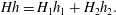
The experimental set-up is shown in figure 2. The 30 cm wide and 5 cm high tank is placed inside a modified microwave oven that achieves a laterally uniform microwave absorption and internal heat release (Surducan et al. Reference Surducan, Surducan, Limare, Neamtu and di Giuseppe2014). The top is made of an aluminium heat exchanger connected to a thermostated bath which allows a constant temperature boundary condition. The bottom boundary is made of a thick poly(methyl-methacrylate) plate which can be considered as adiabatic. The performance of this laboratory set-up was assessed through a thorough comparison with numerical calculations reproducing the exact same configuration, including the tank dimensions and boundary conditions, for a homogeneous fluid layer over a large range of Rayleigh–Roberts numbers (Limare et al. Reference Limare, Vilella, Di Giuseppe, Farnetani, Kaminski, Surducan, Surducan, Neamtu, Fourel and Jaupart2015).
In situ temperature determinations were achieved via laser induced fluorescence (LIF) by adding a combination of two fluorescent dyes in order to separate between composition and temperature contributions to fluorescence. Spatial resolution is set by the 0.2 mm pixel size of the digital camera, enabling excellent resolution of the temperature profile in thermal boundary layers at the top of the tank, which were always thicker than 2 mm. A laser sheet scans half of the tank whilst two CCD cameras acquire images in different spectral ranges, so that temperature and composition can both be measured simultaneously. In addition, a particle image velocimetry system allows determination of the velocity field. Three-dimensional distributions are constructed by interpolation of the two-dimensional data sets. Scans were obtained at a spacing of 1 cm over a half-tank width (15 cm), which allows a representative sampling of the different fields. Dye concentrations in the lower layer are three times larger than in the upper one, which makes for a sharp change of fluorescence between the two fluids and allows us to track the interface that separates them.
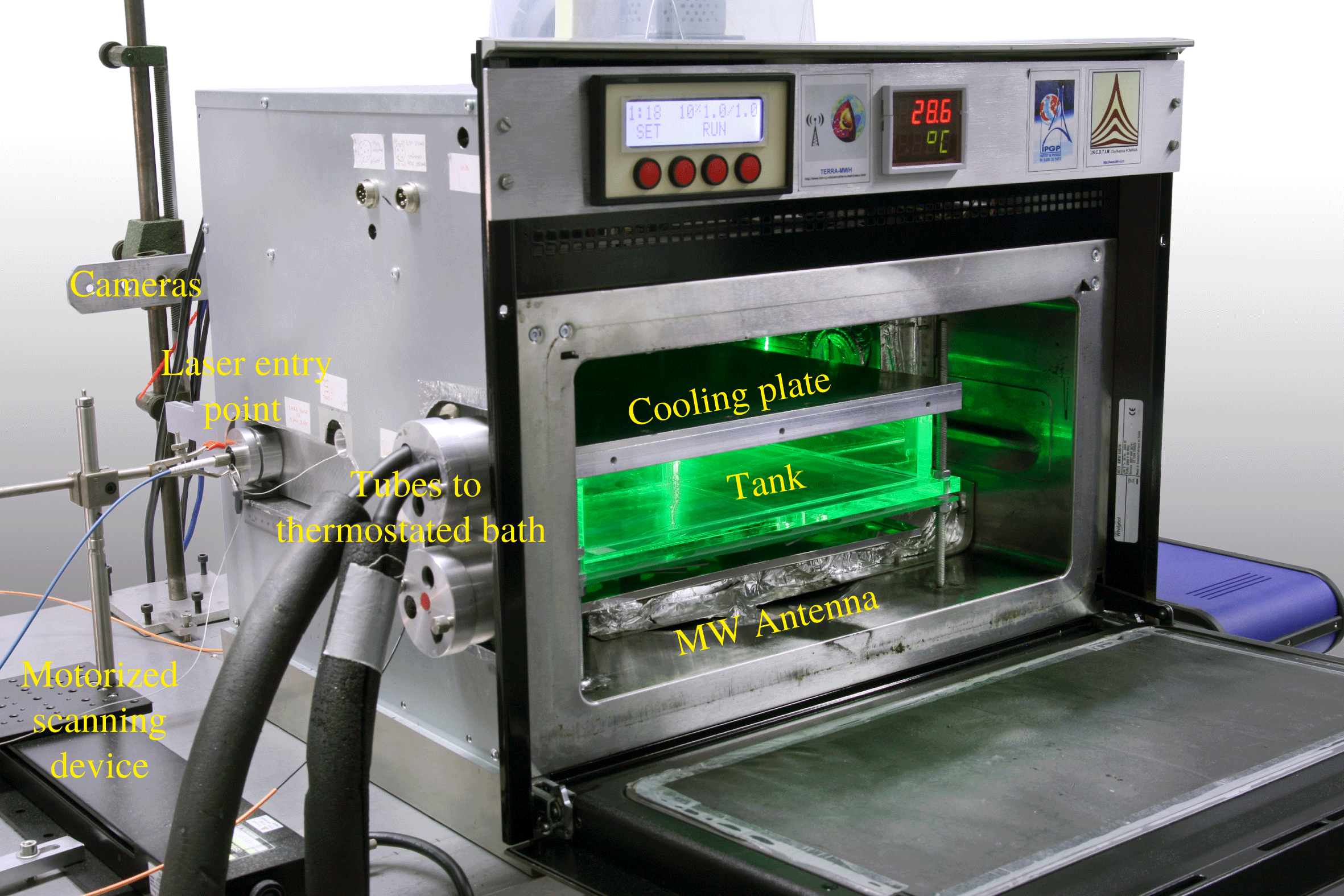
Figure 2. Experimental set-up.
Each experiment followed the same protocol. The fluids were left for at least 12 h in the temperature-controlled laboratory so that they were initially at room temperature. The tank was first completely filled with the upper fluid and air bubbles were carefully removed. Next, a known volume of denser lower layer fluid was injected at the bottom whilst the excess upper fluid was removed. The dense fluid was left to spread across the whole tank and settle in a layer of uniform thickness. This generated an initially stably stratified system. At the start of an experiment, thermostated water at room temperature was made to circulate through the heat exchanger at the top and the microwave source was turned on at some prescribed power. In these conditions, both layers were heating simultaneously at rates that depended on their respective microwave absorption intensities. We did not start by cooling an initially hot initial layer because we sought to avoid an early phase of convection driven exclusively by boundary layer instabilities at the top of the upper fluid independently of internal heat production.
Table 1. List of experiments performed in this study, their dimensionless numbers, their temperature scales and convection regime: domes (D) and stratified (S);
 $B_{cond}$
was obtained using (2.8) with
$B_{cond}$
was obtained using (2.8) with
 $\unicode[STIX]{x0394}T$
the steady-state conduction temperature scale (2.15). Rayleigh numbers are calculated for fluid properties at the volume-averaged temperature, whereas the viscosity ratio is given at a reference temperature (temperature of the top surface).
$\unicode[STIX]{x0394}T$
the steady-state conduction temperature scale (2.15). Rayleigh numbers are calculated for fluid properties at the volume-averaged temperature, whereas the viscosity ratio is given at a reference temperature (temperature of the top surface).
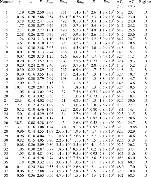
3.2 Experiments
Additional information on fluids properties and other experimental conditions are given in the supplementary material (table S1), available at https://doi.org/10.1017/jfm.2019.243. We performed 38 experiments investigating large ranges of dimensionless numbers (table 1). For the sake of simplicity, we restricted our attention to lower layers that were thinner and with a higher rate of heat generation than the upper one, which is relevant to the undepleted reservoir that is likely to exist at the base of the Earth’s mantle. The lower fluid was allowed to be more and less viscous than the upper one and viscosity contrasts between the two fluids were varied over more than two orders of magnitude (
 $0.06\leqslant \unicode[STIX]{x1D6FE}\leqslant 38$
). We were interested in large Rayleigh–Roberts values appropriate for the Earth’s mantle and did not investigate conditions near the stability threshold. In all experiments
$0.06\leqslant \unicode[STIX]{x1D6FE}\leqslant 38$
). We were interested in large Rayleigh–Roberts values appropriate for the Earth’s mantle and did not investigate conditions near the stability threshold. In all experiments
 $Ra_{2}>Ra_{H1}$
, due to the large impact of the layer thickness on the Rayleigh–Roberts number, a condition that is appropriate for the Earth’s mantle. Based on values of Rayleigh–Roberts number of the lower layer, we investigated cases such that the lower layer would have been able or unable to undergo convection on its own (table 1). Values for the Rayleigh–Roberts for the final homogenized reservoir were in a
$Ra_{2}>Ra_{H1}$
, due to the large impact of the layer thickness on the Rayleigh–Roberts number, a condition that is appropriate for the Earth’s mantle. Based on values of Rayleigh–Roberts number of the lower layer, we investigated cases such that the lower layer would have been able or unable to undergo convection on its own (table 1). Values for the Rayleigh–Roberts for the final homogenized reservoir were in a
 $3\times 10^{4}-5\times 10^{7}$
range, which straddles the threshold between steady and time-dependent convection regimes (Vilella et al.
Reference Vilella, Limare, Jaupart, Farnetani, Fourel and Kaminski2018).
$3\times 10^{4}-5\times 10^{7}$
range, which straddles the threshold between steady and time-dependent convection regimes (Vilella et al.
Reference Vilella, Limare, Jaupart, Farnetani, Fourel and Kaminski2018).
4 Thermal structure and heat flux through the upper boundary
4.1 Time evolution
All experiments followed the same basic evolution, with an interface that started to deform when convection set in. The volume of lower fluid separated from the upper fluid by a well-defined interface decreased steadily until there was no longer evidence for the existence of two different fluid regions in the tank. We describe later how the interface deformed and how mingling proceeded and discuss here the evolution of convection from a purely thermal perspective.
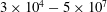
We derived vertical profiles of the horizontally averaged temperature and calculated the heat flux at the top of the tank using a least-squares linear fit to the three uppermost temperature values. Figure 3 shows how the vertical profile of the horizontally averaged temperature changes with time for experiment 21. At small times, the profiles bear the influence of two different fluid layers, with an upper region that appears well mixed beneath an upper boundary layer and a lower region with a large negative temperature gradient. Later in the experiment, there is little evidence for a basal fluid layer, which is due to the large deformations of the interface, such that the lower fluid is not confined below a well-defined horizon (as later shown in § 5.2). With increasing time, upper regions warm up whilst lower ones cool down until a steady-state profile with the hallmarks of an internally heated fluid layer is achieved, with a small but well-defined stable temperature gradient in the fluid interior (Vilella et al. Reference Vilella, Limare, Jaupart, Farnetani, Fourel and Kaminski2018). This late evolution proceeds by changes of internal thermal structure that maintain the volume-average temperature and the heat flux at the top almost constant. At these late times, there is no longer a lower layer at the base but one can still observe thin slivers of lower fluid in the tank interior. There is no detectable heterogeneity at the scale of the fluid motions and the reservoir can be considered as both homogeneous from a thermal standpoint and heterogeneous from a chemical standpoint.
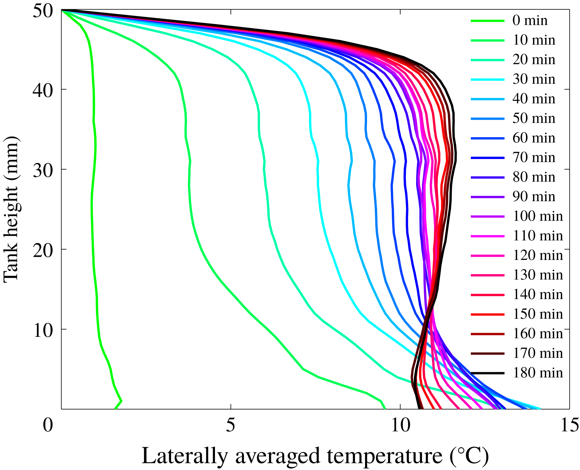
Figure 3. Vertical profiles of the horizontally averaged temperature as a function of time for experiment 21. Colours indicate time evolution from green to blue, red and black. Profiles are taken every 10 min from green (0 min) to blue, red and black (180 min). The profiles tend to that for a homogeneous fluid layer in equilibrium with its heat sources, with a small stable interior bulk thermal stratification.
We have tracked the time evolution of convection using the heat flux
 $\unicode[STIX]{x1D719}$
at the top and the volume-averaged temperature in the tank
$\unicode[STIX]{x1D719}$
at the top and the volume-averaged temperature in the tank
 $\langle T\rangle$
(figure 4). Both variables tended towards steady-state values, noted
$\langle T\rangle$
(figure 4). Both variables tended towards steady-state values, noted
 $\unicode[STIX]{x1D719}_{\infty }$
and
$\unicode[STIX]{x1D719}_{\infty }$
and
 $T_{vol}$
, over a well-defined time. There were small and simultaneous fluctuations in both the heat flux and temperature records, which will be discussed later. At steady state, the heat flux at the top was equal to the total amount of heat released in the tank interior, as required in equilibrium conditions.
$T_{vol}$
, over a well-defined time. There were small and simultaneous fluctuations in both the heat flux and temperature records, which will be discussed later. At steady state, the heat flux at the top was equal to the total amount of heat released in the tank interior, as required in equilibrium conditions.
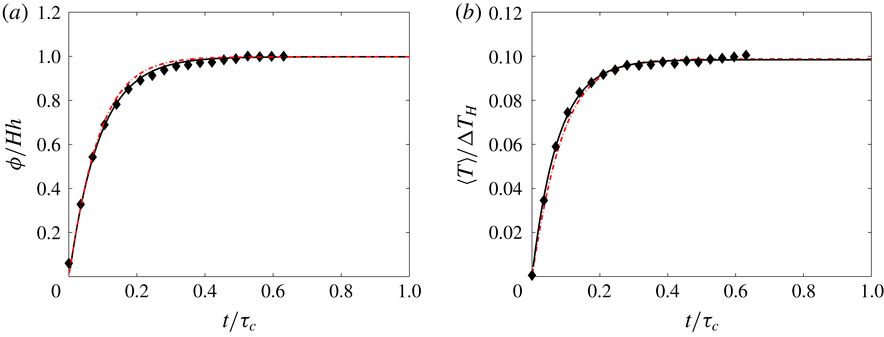
Figure 4. Dimensionless heat flux (a) and volume-averaged temperature (b) as a function of time normalized to the conduction time for the whole layer,
 $\unicode[STIX]{x1D70F}_{c}=h^{2}/\unicode[STIX]{x1D705}$
, for experiment 21. Black diamonds represent experimental data, black lines represent exponential fits and red, dashed lines represent the results of transient calculations from (4.3) and (4.5).
$\unicode[STIX]{x1D70F}_{c}=h^{2}/\unicode[STIX]{x1D705}$
, for experiment 21. Black diamonds represent experimental data, black lines represent exponential fits and red, dashed lines represent the results of transient calculations from (4.3) and (4.5).
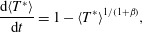
To demonstrate that the apparent thermal steady state corresponds to that of a homogeneous fluid, we checked that the two thermal structures conform to the same scaling laws. This is evaluated in figure 5, where the steady-state volume-averaged temperature
 $T_{vol}$
is shown as a function of the ‘bulk’ Rayleigh–Roberts number
$T_{vol}$
is shown as a function of the ‘bulk’ Rayleigh–Roberts number
 $Ra_{H}$
(4.1). Also shown in this figure are data from experiments in homogeneous fluids published in a previous study (Limare et al.
Reference Limare, Vilella, Di Giuseppe, Farnetani, Kaminski, Surducan, Surducan, Neamtu, Fourel and Jaupart2015) and listed in the supplementary material in table S2. At large values of
$Ra_{H}$
(4.1). Also shown in this figure are data from experiments in homogeneous fluids published in a previous study (Limare et al.
Reference Limare, Vilella, Di Giuseppe, Farnetani, Kaminski, Surducan, Surducan, Neamtu, Fourel and Jaupart2015) and listed in the supplementary material in table S2. At large values of
 $Ra_{H}$
(
$Ra_{H}$
(
 ${>}10^{5}$
), Vilella et al. (Reference Vilella, Limare, Jaupart, Farnetani, Fourel and Kaminski2018) have shown that the two variables are related to one another by the following scaling law:
${>}10^{5}$
), Vilella et al. (Reference Vilella, Limare, Jaupart, Farnetani, Fourel and Kaminski2018) have shown that the two variables are related to one another by the following scaling law:
 $$\begin{eqnarray}\displaystyle {\displaystyle \frac{T_{vol}}{\unicode[STIX]{x0394}T_{H}}}=CRa_{H}^{\unicode[STIX]{x1D6FD}}, & & \displaystyle\end{eqnarray}$$
with an exponent
 $\unicode[STIX]{x1D6FD}$
close to the value of
$\unicode[STIX]{x1D6FD}$
close to the value of
 $-1/4$
for Boussinesq fluids with constant physical properties (table 3);
$-1/4$
for Boussinesq fluids with constant physical properties (table 3);
 $C$
is a constant depending on the mechanical boundary conditions, rigid in our case. Within their error ranges, best-fit values of the two parameters in the scaling law are equal to those for homogeneous fluids. Moreover, they are almost identical to those obtained numerically in isoviscous and infinite Prandtl fluids encased in tanks with rigid walls (Vilella et al.
Reference Vilella, Limare, Jaupart, Farnetani, Fourel and Kaminski2018) (table 3).
$C$
is a constant depending on the mechanical boundary conditions, rigid in our case. Within their error ranges, best-fit values of the two parameters in the scaling law are equal to those for homogeneous fluids. Moreover, they are almost identical to those obtained numerically in isoviscous and infinite Prandtl fluids encased in tanks with rigid walls (Vilella et al.
Reference Vilella, Limare, Jaupart, Farnetani, Fourel and Kaminski2018) (table 3).
Figure 5. Dimensionless steady-state volume-averaged temperature as a function of Rayleigh–Roberts number: black diamonds represent data from this study (heterogeneous convection experiments) and empty squares data from experiments in homogeneous fluids (Limare et al. Reference Limare, Vilella, Di Giuseppe, Farnetani, Kaminski, Surducan, Surducan, Neamtu, Fourel and Jaupart2015). Lines represent fits obtained with a fixed exponent (table 3); heterogeneous (full line) and homogeneous (dashed line).
Table 2. List of experiments performed in this study, their characteristic volume-average temperatures and time constants.
 $T_{vol}$
is the steady-state volumetrically averaged temperature and
$T_{vol}$
is the steady-state volumetrically averaged temperature and
 $\unicode[STIX]{x1D70F}_{e}$
is the thermal relaxation time according to (4.6);
$\unicode[STIX]{x1D70F}_{e}$
is the thermal relaxation time according to (4.6);
 $T_{12\,max}$
is the maximum value of the volume-average temperature contrast between the two layers and
$T_{12\,max}$
is the maximum value of the volume-average temperature contrast between the two layers and
 $\unicode[STIX]{x1D70F}_{12\,max}$
is the time at which this maximum occurs.
$\unicode[STIX]{x1D70F}_{12\,max}$
is the time at which this maximum occurs.

Table 3. Parameters of empirical best-fit power laws for the volume-average (
 $T_{vol}/\unicode[STIX]{x0394}T_{H}$
) temperature in steady state at high values of the Rayleigh–Roberts number (
$T_{vol}/\unicode[STIX]{x0394}T_{H}$
) temperature in steady state at high values of the Rayleigh–Roberts number (
 $Ra_{H}\geqslant 10^{5}$
) for heterogeneous and homogeneous laboratory experiments. Data for homogeneous fluid layers are taken from the experiments by Limare et al. (Reference Limare, Vilella, Di Giuseppe, Farnetani, Kaminski, Surducan, Surducan, Neamtu, Fourel and Jaupart2015).
$Ra_{H}\geqslant 10^{5}$
) for heterogeneous and homogeneous laboratory experiments. Data for homogeneous fluid layers are taken from the experiments by Limare et al. (Reference Limare, Vilella, Di Giuseppe, Farnetani, Kaminski, Surducan, Surducan, Neamtu, Fourel and Jaupart2015).
In the final steady state, the convective heat flux at the top evacuates all the heat released within the layer. Thus, equation (4.1) for the volume-averaged temperature can be turned into an equation for the heat flux at the top noted
 $\unicode[STIX]{x1D719}_{\infty }$
:
$\unicode[STIX]{x1D719}_{\infty }$
:
 $$\begin{eqnarray}\displaystyle \unicode[STIX]{x1D719}_{\infty }=\left({\displaystyle \frac{k}{Ch}}\right)^{1/(1+\unicode[STIX]{x1D6FD})}\left({\displaystyle \frac{g\unicode[STIX]{x1D6FC}\unicode[STIX]{x1D70C}h^{4}}{k\unicode[STIX]{x1D705}\unicode[STIX]{x1D707}}}\right)^{-\unicode[STIX]{x1D6FD}/(1+\unicode[STIX]{x1D6FD})}T_{vol}^{1/(1+\unicode[STIX]{x1D6FD})}. & & \displaystyle\end{eqnarray}$$
This heat flux is transported by conduction through the upper unstable boundary layer. We note that, for
 $\unicode[STIX]{x1D6FD}=-1/4$
,
$\unicode[STIX]{x1D6FD}=-1/4$
,
 $\unicode[STIX]{x1D719}_{\infty }\propto T_{vol}^{4/3}$
and the total fluid thickness
$\unicode[STIX]{x1D719}_{\infty }\propto T_{vol}^{4/3}$
and the total fluid thickness
 $h$
gets cancelled in this expression. In this case, the dynamics of the upper boundary layer is controlled locally, independently of the deep fluid region below. As shown by Vilella et al. (Reference Vilella, Limare, Jaupart, Farnetani, Fourel and Kaminski2018), the volume-averaged temperature
$h$
gets cancelled in this expression. In this case, the dynamics of the upper boundary layer is controlled locally, independently of the deep fluid region below. As shown by Vilella et al. (Reference Vilella, Limare, Jaupart, Farnetani, Fourel and Kaminski2018), the volume-averaged temperature
 $T_{vol}$
and the temperature difference across the upper boundary layer, noted
$T_{vol}$
and the temperature difference across the upper boundary layer, noted
 $\unicode[STIX]{x0394}T_{TBL}$
, are both scaled to
$\unicode[STIX]{x0394}T_{TBL}$
, are both scaled to
 $Ra_{H}^{-1/4}$
, so that
$Ra_{H}^{-1/4}$
, so that
 $\unicode[STIX]{x1D719}_{\infty }\propto \unicode[STIX]{x0394}T_{TBL}^{4/3}$
, which conforms to the well-known local heat flux law for actively convecting layers (Townsend Reference Townsend1964).
$\unicode[STIX]{x1D719}_{\infty }\propto \unicode[STIX]{x0394}T_{TBL}^{4/3}$
, which conforms to the well-known local heat flux law for actively convecting layers (Townsend Reference Townsend1964).
4.2 Transient thermal evolution
The transient thermal evolution of the whole fluid is governed by the heat balance equation:
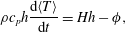 $$\begin{eqnarray}\displaystyle \unicode[STIX]{x1D70C}c_{p}h{\displaystyle \frac{\text{d}\langle T\rangle }{\text{d}t}}=Hh-\unicode[STIX]{x1D719}, & & \displaystyle\end{eqnarray}$$
where
 $\langle T\rangle$
and
$\langle T\rangle$
and
 $\unicode[STIX]{x1D719}$
are the time-dependent volume-averaged temperature and heat flux at the top of the tank, respectively. This equation can also be rewritten as an equation for the heat flux, which evacuates heat produced internally as well as sensible heat extracted through cooling (appearing as
$\unicode[STIX]{x1D719}$
are the time-dependent volume-averaged temperature and heat flux at the top of the tank, respectively. This equation can also be rewritten as an equation for the heat flux, which evacuates heat produced internally as well as sensible heat extracted through cooling (appearing as
 $-\unicode[STIX]{x1D70C}c_{p}(\text{d}\langle T\rangle /\text{d}t)$
). In transient conditions, the unstable boundary layer at the top is much thinner than the whole fluid and rapidly adjusts to the interior thermal structure. One can thus assume that the local heat flux expression (4.2) remains valid at all times as a function of the instantaneous value of the volume-averaged temperature
$-\unicode[STIX]{x1D70C}c_{p}(\text{d}\langle T\rangle /\text{d}t)$
). In transient conditions, the unstable boundary layer at the top is much thinner than the whole fluid and rapidly adjusts to the interior thermal structure. One can thus assume that the local heat flux expression (4.2) remains valid at all times as a function of the instantaneous value of the volume-averaged temperature
 $\langle T\rangle$
(figure 3). This standard and well-tested approximation was validated by the careful laboratory experiments of Katsaros et al. (Reference Katsaros, Liu, Businger and Tillman1977). Scaling temperature by the steady-state value
$\langle T\rangle$
(figure 3). This standard and well-tested approximation was validated by the careful laboratory experiments of Katsaros et al. (Reference Katsaros, Liu, Businger and Tillman1977). Scaling temperature by the steady-state value
 $T_{vol}$
in the heat balance equation leads to the following time scale:
$T_{vol}$
in the heat balance equation leads to the following time scale:
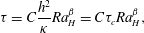 $$\begin{eqnarray}\displaystyle \unicode[STIX]{x1D70F}=C{\displaystyle \frac{h^{2}}{\unicode[STIX]{x1D705}}}Ra_{H}^{\unicode[STIX]{x1D6FD}}=C\unicode[STIX]{x1D70F}_{c}Ra_{H}^{\unicode[STIX]{x1D6FD}}, & & \displaystyle\end{eqnarray}$$
where
 $\unicode[STIX]{x1D70F}_{c}=h^{2}/\unicode[STIX]{x1D705}$
is the diffusive time scale for the whole fluid layer. Using these scales, the dimensionless heat balance equation is:
$\unicode[STIX]{x1D70F}_{c}=h^{2}/\unicode[STIX]{x1D705}$
is the diffusive time scale for the whole fluid layer. Using these scales, the dimensionless heat balance equation is:
 $$\begin{eqnarray}\displaystyle {\displaystyle \frac{\text{d}\langle T^{\ast }\rangle }{\text{d}t}}=1-\langle T^{\ast }\rangle ^{1/(1+\unicode[STIX]{x1D6FD})}, & & \displaystyle\end{eqnarray}$$
where
 $\langle T^{\ast }\rangle =\langle T\rangle /T_{vol}$
is the dimensionless volume-averaged temperature. Integrating this equation, we find that calculated values of the heat flux and volume-averaged temperature are very close to the measured ones at all times (figure 4).
$\langle T^{\ast }\rangle =\langle T\rangle /T_{vol}$
is the dimensionless volume-averaged temperature. Integrating this equation, we find that calculated values of the heat flux and volume-averaged temperature are very close to the measured ones at all times (figure 4).
The agreement between data and model predictions that is shown in figure 4 is obtained for an experiment with a low
 $B$
value and a relatively large
$B$
value and a relatively large
 $Ra_{H}$
value (experiment 21, table 1). We have checked that this is true for all experiments. In particular, we show results for an experiment with a high
$Ra_{H}$
value (experiment 21, table 1). We have checked that this is true for all experiments. In particular, we show results for an experiment with a high
 $B$
value and a low
$B$
value and a low
 $Ra_{H}$
value (experiment 10) in the supplementary material (figure S1). Differences between the experimental data and the theoretical predictions are slightly larger than for experiments at larger values of
$Ra_{H}$
value (experiment 10) in the supplementary material (figure S1). Differences between the experimental data and the theoretical predictions are slightly larger than for experiments at larger values of
 $Ra_{H}$
. This is expected because the
$Ra_{H}$
. This is expected because the
 $\unicode[STIX]{x1D719}_{\infty }-T_{vol}$
scaling law with power-law exponent
$\unicode[STIX]{x1D719}_{\infty }-T_{vol}$
scaling law with power-law exponent
 $\unicode[STIX]{x1D6FD}=-1/4$
is only valid for
$\unicode[STIX]{x1D6FD}=-1/4$
is only valid for
 $Ra_{H}>6\times 10^{5}$
(Limare et al.
Reference Limare, Vilella, Di Giuseppe, Farnetani, Kaminski, Surducan, Surducan, Neamtu, Fourel and Jaupart2015; Vilella et al.
Reference Vilella, Limare, Jaupart, Farnetani, Fourel and Kaminski2018), such that the upper boundary layer is very much thinner than the reservoir. Deviations of
$Ra_{H}>6\times 10^{5}$
(Limare et al.
Reference Limare, Vilella, Di Giuseppe, Farnetani, Kaminski, Surducan, Surducan, Neamtu, Fourel and Jaupart2015; Vilella et al.
Reference Vilella, Limare, Jaupart, Farnetani, Fourel and Kaminski2018), such that the upper boundary layer is very much thinner than the reservoir. Deviations of
 $T_{vol}$
from this scaling account for most of the scatter in figure 5. In order to verify further that the experimental data are consistent with these scalings, we have determined the duration of the thermal transient, independently of any model calculation or scaling. One procedure would consist of setting a threshold value for either the heat flux or volume-averaged temperature at some fraction of their final steady-state values and determining the times when this is reached. Results depend on the rather arbitrarily chosen threshold and on the accuracy of temperature determinations, therefore we used another method. The evolution of both the heat flux and the volume-averaged temperature seem to be very close to a simple exponential relaxation (figure 4). This allows the determination of a characteristic time
$T_{vol}$
from this scaling account for most of the scatter in figure 5. In order to verify further that the experimental data are consistent with these scalings, we have determined the duration of the thermal transient, independently of any model calculation or scaling. One procedure would consist of setting a threshold value for either the heat flux or volume-averaged temperature at some fraction of their final steady-state values and determining the times when this is reached. Results depend on the rather arbitrarily chosen threshold and on the accuracy of temperature determinations, therefore we used another method. The evolution of both the heat flux and the volume-averaged temperature seem to be very close to a simple exponential relaxation (figure 4). This allows the determination of a characteristic time
 $\unicode[STIX]{x1D70F}_{e}$
such that, for example, the time-dependent heat flux is:
$\unicode[STIX]{x1D70F}_{e}$
such that, for example, the time-dependent heat flux is:
 $$\begin{eqnarray}\displaystyle \unicode[STIX]{x1D719}(t)=Hh(1-\text{e}^{-t/\unicode[STIX]{x1D70F}_{e}}). & & \displaystyle\end{eqnarray}$$
The exponential approximation of (4.6) allows a very good fit to the experimental data (figure 4
a) and we have determined
 $\unicode[STIX]{x1D70F}_{e}$
values for all experiments through a best-fit procedure. With this method, we can use both the temperature and heat flux data, and we can assess the overall trend towards equilibrium. Further, substituting for this approximate expression in the bulk heat balance equation leads to a very good agreement with the temperature measurements (figure 4
b). If the above scaling arguments are correct,
$\unicode[STIX]{x1D70F}_{e}$
values for all experiments through a best-fit procedure. With this method, we can use both the temperature and heat flux data, and we can assess the overall trend towards equilibrium. Further, substituting for this approximate expression in the bulk heat balance equation leads to a very good agreement with the temperature measurements (figure 4
b). If the above scaling arguments are correct,
 $\unicode[STIX]{x1D70F}_{e}$
should scale with
$\unicode[STIX]{x1D70F}_{e}$
should scale with
 $\unicode[STIX]{x1D70F}_{c}Ra_{H}^{\unicode[STIX]{x1D6FD}}$
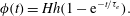
, which is tested successfully in figure 6 and table 4. For convenience, we shall use the value of
$\unicode[STIX]{x1D70F}_{c}Ra_{H}^{\unicode[STIX]{x1D6FD}}$
, which is tested successfully in figure 6 and table 4. For convenience, we shall use the value of
 $\unicode[STIX]{x1D6FD}=-1/4$
throughout the paper, rather than some empirical value within an uncertainty range.
$\unicode[STIX]{x1D6FD}=-1/4$
throughout the paper, rather than some empirical value within an uncertainty range.
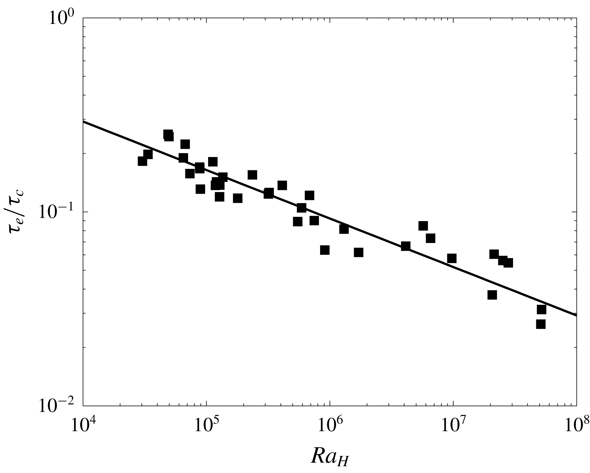
Figure 6. Dimensionless thermal relaxation time
 $\unicode[STIX]{x1D70F}_{e}/\unicode[STIX]{x1D70F}_{c}$
for convection as a function of the bulk Rayleigh–Roberts number
$\unicode[STIX]{x1D70F}_{e}/\unicode[STIX]{x1D70F}_{c}$
for convection as a function of the bulk Rayleigh–Roberts number
 $Ra_{H}$
. Line represents the fit obtained by setting the power-law exponent to the value of
$Ra_{H}$
. Line represents the fit obtained by setting the power-law exponent to the value of
 $-1/4$
(table 4).
$-1/4$
(table 4).
Table 4. Parameters of empirical best-fit power laws for the characteristic time constant
 $\unicode[STIX]{x1D70F}_{e}$
.
$\unicode[STIX]{x1D70F}_{e}$
.
For planetary studies, the important implication is that the bulk thermal evolution of a planet (which is usually referred to as ‘secular cooling’) is not sensitive to the exact distribution of its internal heat sources, for reasons that will be explained below. As shown below, however, other features of convection, such as planforms and distribution and size of upwellings, depend on the distribution of heat sources as well as on differences in the properties of the two fluids.
5 Two different convection regimes
The topography of the interface that separates the two fluids provides a natural marker of flow structure and is of particular interest for comparison with tomographic images of the Earth’s mantle. As argued by Fourel et al. (Reference Fourel, Limare, Jaupart, Surducan, Farnetani, Kaminski, Neamtu and Surducan2017), deformation is both a consequence and a driver of convective motions due to enhanced heat generation in the lower fluid. The interface is well defined initially because it is characterized by an almost step change of composition and transmitted light intensity. As time progresses, however, mixing of the two fluids is generated at the interface which therefore becomes blurred. We identify an interface when there is a core of lower fluid with a composition that is close to the initial value. Such a core is separated from neighbouring fluid by a sharp composition gradient and we locate the interface using a threshold composition value. Due to the sharp gradient, the position of the interface is weakly sensitive to the exact threshold value that is adopted, as shown in the supplementary material. At large distances from core regions, thin threads of lower fluid can survive for very long times but they are distributed through large volumes and do not affect the fluid motion. In these conditions, they behave as passive tracers (see § 6.1).
In all our experiments, there was some entrainment of upper fluid into the lower fluid, as described later, but it was the upper fluid that ended up ingesting all the lower fluid. In principle, mixing could proceed the other way around with the lower fluid engulfing increasing amounts of upper fluid until the mixture occupies the whole tank. This did not happen in the present set of experiments because convective motions are systematically more intense in the upper layer, due to the higher Rayleigh–Roberts number.
The interface topography is defined as the distribution of interface height above the tank base and develops in two different regimes which can be understood using two end-member cases. For a small density and viscosity contrasts, the interface does not act as a barrier and deforms passively, such that the two fluids undergo convective motions that are determined at the scale of the whole tank (‘doming’ regime). For large values of the density contrast, the interface remains flat but mixing still occurs, due to the shearing and extraction of thin slivers of lower fluid (‘stratified’ regime). In principle, one should differentiate between mixing and mingling although they are parts of the same process in miscible fluids. They both describe the entrainment of one fluid into the other, which proceeds in two different ways. One is such that one fluid protrudes into the other and folds over, engulfing parts of the other fluid. In the other process, shear at the interface acts to tear a thin schlieren out of one fluid. These two processes are involved to different degrees in the two regimes of interface deformation. They are both such that entrained fluid parcels get stretched and thinned, up to a point when diffusion becomes effective and eradicates composition differences. Mixing applies to this whole sequence and mingling describes the intermediate process of generating small parcels of one fluid that get carried by the other one. Mingling leads to mixtures that are heterogeneous at a local scale and yet can be homogeneous at large scales.
5.1 The stratified regime
All else being equal, this regime is observed for intrinsically denser lower fluids than in the dome regime, which prevents large-scale protrusions of lower fluid into the upper one (movie 2 in supplementary material). Figure 7 shows three different snapshots of the flow structure, which document the topography of the lower layer together with the horizontal distribution of the average vertical velocity field in each layer. The interface develops a morphology of cusp-like ridges encircling basins. The basins grow deeper with time and eventually extend to the base of the tank, which becomes exposed to the upper fluid in several locations. These areas gradually widen until they occupy the whole base of the tank. The cusps that delimit the basins are due to converging flows feeding upwellings in the upper fluid, whereas the basins are associated with downwellings (figure 7).
Figure 7. Interface topography and distribution of the average vertical velocity above and below the interface at
 $t=40~\text{min}$
(a), 100 min (b) and 160 min (c) for experiment 7 in the stratified regime. Space dimensions are in mm.
$t=40~\text{min}$
(a), 100 min (b) and 160 min (c) for experiment 7 in the stratified regime. Space dimensions are in mm.
The cusp and basin morphology of the interface leads to a peaked probability density function (PDF) for the interface height with a long thinning tail at high values. In order to characterize these functions in a quantitative manner, we use gamma distributions:
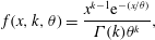 $$\begin{eqnarray}\displaystyle f(x,k,\unicode[STIX]{x1D703})={\displaystyle \frac{x^{k-1}\text{e}^{-(x/\unicode[STIX]{x1D703})}}{\unicode[STIX]{x1D6E4}(k)\unicode[STIX]{x1D703}^{k}}}, & & \displaystyle\end{eqnarray}$$
where
 $\unicode[STIX]{x1D6E4}$
stands for the gamma function,
$\unicode[STIX]{x1D6E4}$
stands for the gamma function,
 $\unicode[STIX]{x1D703}$
is a scale factor and
$\unicode[STIX]{x1D703}$
is a scale factor and
 $k$
is a parameter. As shown in figure 8, these distributions allow a good fit to the experimental data, as shown by the very large values of the correlation coefficient (
$k$
is a parameter. As shown in figure 8, these distributions allow a good fit to the experimental data, as shown by the very large values of the correlation coefficient (
 $R>0.99$
). More importantly, these distributions allow us to track how the distribution changes with time. At
$R>0.99$
). More importantly, these distributions allow us to track how the distribution changes with time. At
 $t=0~\text{min}$
, one would expect the cumulative distribution (CDF) to be a step function, corresponding to a perfectly flat interface between the two layers. At that initial recording time, the interface has already developed undulations and the height distribution shows up as a narrow peak, close to ‘normal’ distribution, which is the limiting form of the gamma distribution at large values of
$t=0~\text{min}$
, one would expect the cumulative distribution (CDF) to be a step function, corresponding to a perfectly flat interface between the two layers. At that initial recording time, the interface has already developed undulations and the height distribution shows up as a narrow peak, close to ‘normal’ distribution, which is the limiting form of the gamma distribution at large values of
 $k$
. With time, as the cusp and basin morphology develops, the distribution changes and the
$k$
. With time, as the cusp and basin morphology develops, the distribution changes and the
 $k$
parameter decreases steadily from an initial value of 150, to a value of 10 at
$k$
parameter decreases steadily from an initial value of 150, to a value of 10 at
 $t=40~\text{min}$
and then to 4.5 at
$t=40~\text{min}$
and then to 4.5 at
 $t=100~\text{min}$
. At large times, the distribution is close to ‘exponential’, which is the limiting form of the gamma distribution for
$t=100~\text{min}$
. At large times, the distribution is close to ‘exponential’, which is the limiting form of the gamma distribution for
 $k=1$
. At
$k=1$
. At
 $t=160~\text{min}$
, for example, the best-fit
$t=160~\text{min}$
, for example, the best-fit
 $k$
value is 1.2 (figure 8).
$k$
value is 1.2 (figure 8).
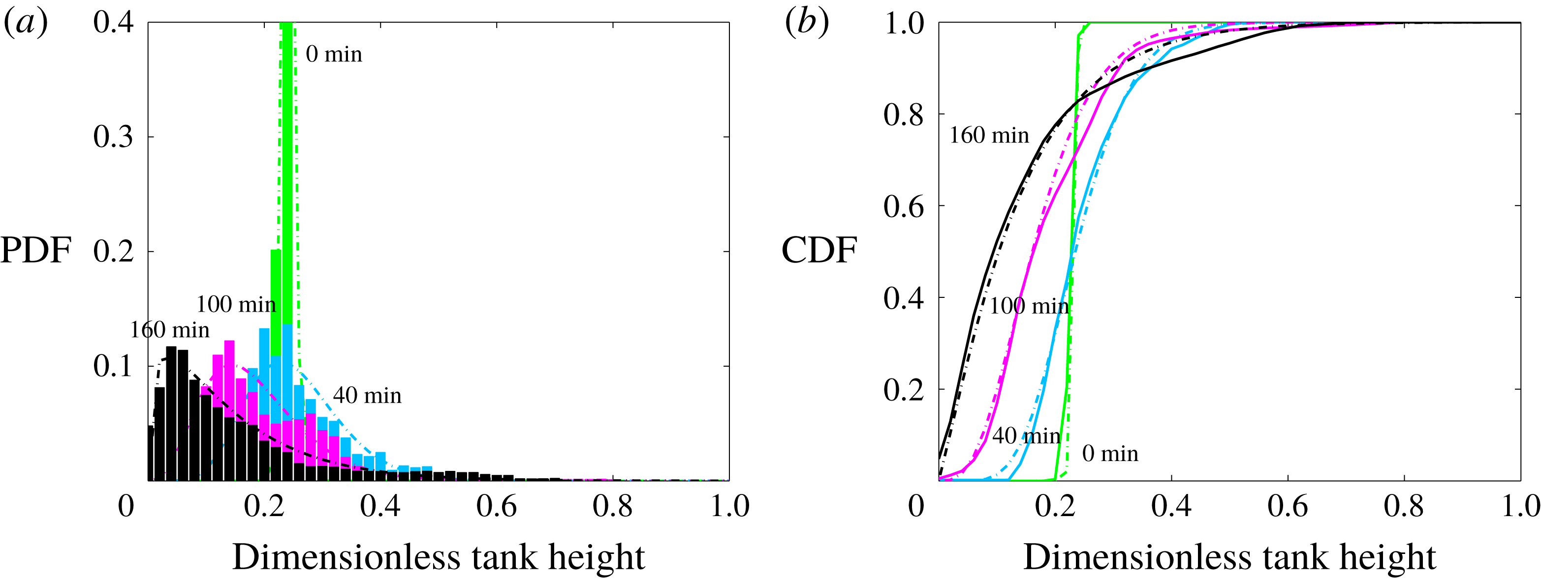
Figure 8. Probability density function (a), cumulative density function (b) of the interface height at different times for experiment 7 in the stratified regime. Dashed line indicate gamma distribution function fits.
5.2 The doming regime
We illustrate the characteristics of the dome regime using experiment 21 (table 1, movie 1 in supplementary material). In this regime, large domal structures grow steadily into columns that eventually reach the top of the tank. As they rise through the tank, these structures lose heat to the colder surroundings but do not fall back down readily as in Rayleigh–Bénard experiments (Davaille Reference Davaille1999b ; Davaille, Le Bars & Carbonne Reference Davaille, Le Bars and Carbonne2003; Le Bars & Davaille Reference Le Bars and Davaille2004a ,Reference Le Bars and Davaille b ). This is because they are made of lower fluid with a higher than average heat production rate, which sustains a temperature difference with the surrounding fluid. In some cases, the domes do deflate and go down, but they do not do so over a large depth range, which sets this behaviour apart from the ‘lava lamp’ oscillatory regime of double-diffusive convection (Turner Reference Turner1974).
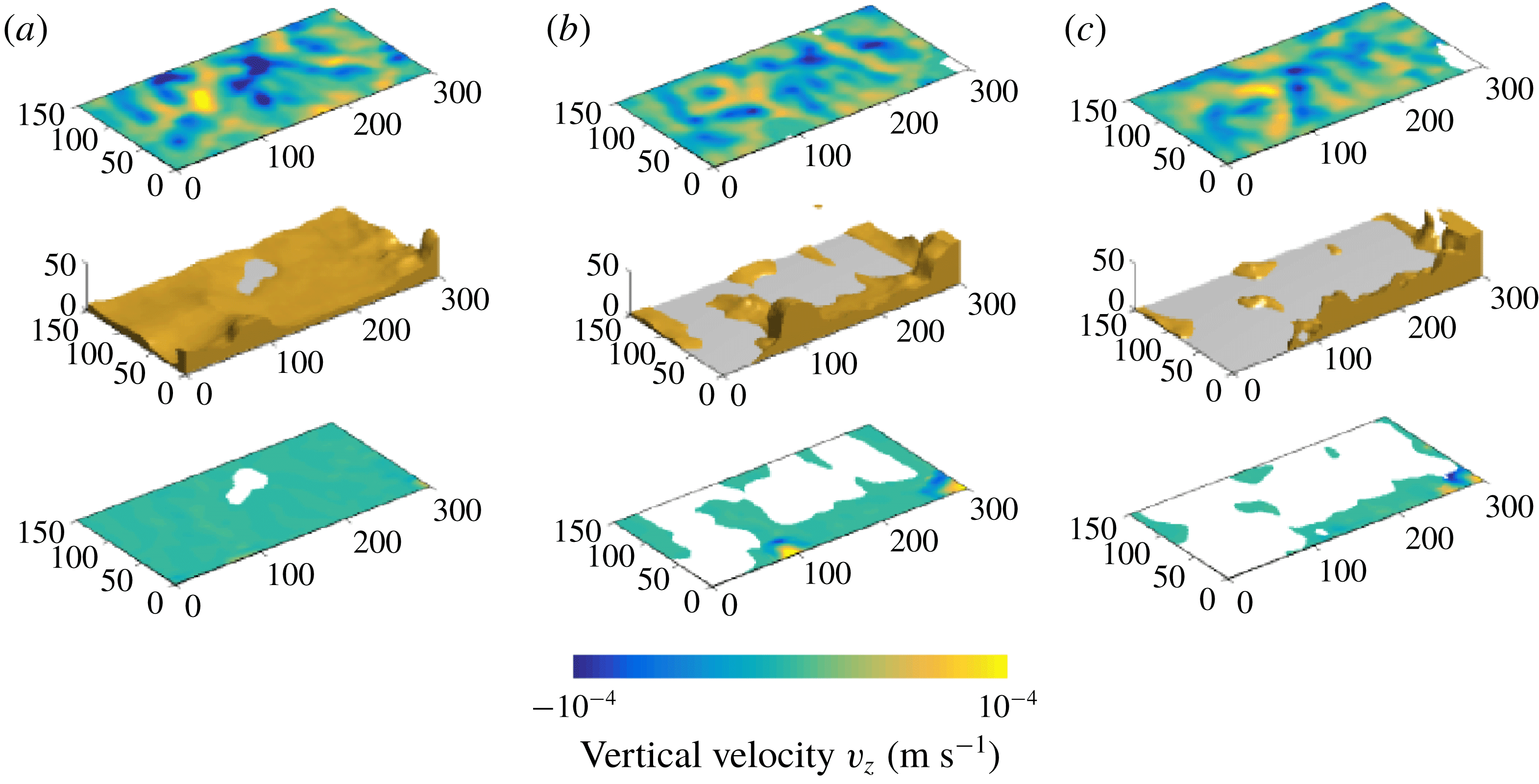
Figure 9. Snapshots of the convective flow structure at three different times (a) 40 min (b) 90 min and (c) 130 min for experiment 21 in the dome regime. Three different types of data are shown at each time. The middle figure shows the interface topography, with grey areas indicating where the lower layer has been thinned to zero. The top and lower figure show the horizontal distribution of the averaged vertical velocity in the upper and lower fluids, respectively. Space dimensions are in mm.
In experiment 21, convection develops first in the upper layer (figure 9 a, top map) and acts to deform the lower layer. An internal circulation develops within the large domes, with a central upwelling surrounded by a peripheral downwelling (visible in the bottom part of figure 9 b). This contrasts with the flow pattern in a homogeneous internally heated layer, which is characterized by narrow downwellings and a diffuse upward return flow (Vilella et al. Reference Vilella, Limare, Jaupart, Farnetani, Fourel and Kaminski2018). Here, the upwellings of the upper layer get localized at the edges of the domes (figure 9 b,c).
Figure 10 shows both the probability density function (PDF) and the cumulative density function (CDF) of the interface height. The interface is almost flat initially, such that the PDF is normal with a narrow peak and a small standard deviation. As convection develops, the PDF becomes increasingly asymmetrical (blue: 30 min and magenta: 60 min) with a peak that widens and eventually disappears (black curve). The gradual change of interface deformation is perhaps better illustrated by the cumulative density function (figure 10 b), which starts as a step function and tends towards a linear function spanning the whole interval. These changes reflect the steady upward growth of domes which eventually stretch over the whole tank thickness.
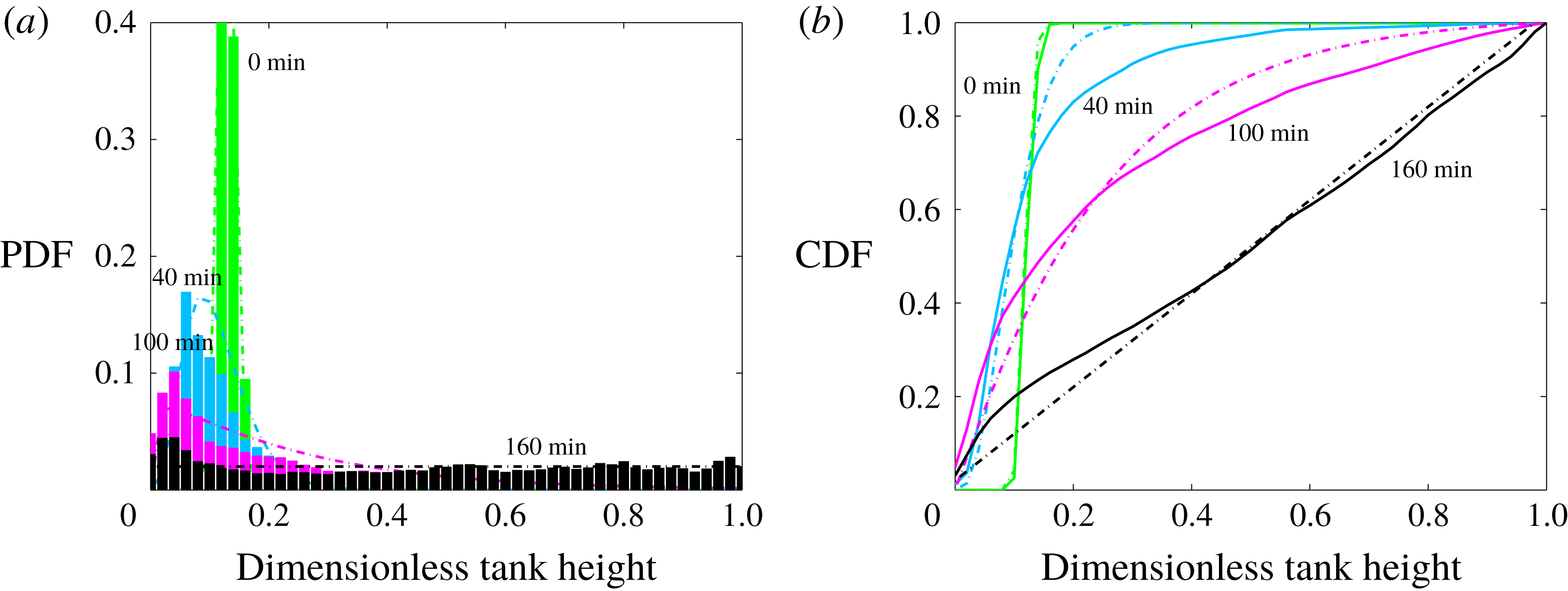
Figure 10. Probability density function (a), cumulative density function (b) of the interface height at different times for experiment 21 in the dome regime. Dashed lines indicate gamma distribution function fits except for
 $t=160~\text{min}$
(uniform distribution).
$t=160~\text{min}$
(uniform distribution).
The domes are large-scale coherent structures made of weakly diluted lower fluid which stands in upper fluid and gets sheared out in thin slivers. We shall document later how mixing proceeds and limit ourselves to the dome dimensions. The domes evolve into nearly cylindrical columns with diameters that barely change with height above the base and remain stable for extended lengths of time (figure 11). Stable dome diameters at mid-height in the reservoir scale approximately with the lower layer thickness (figure 12).
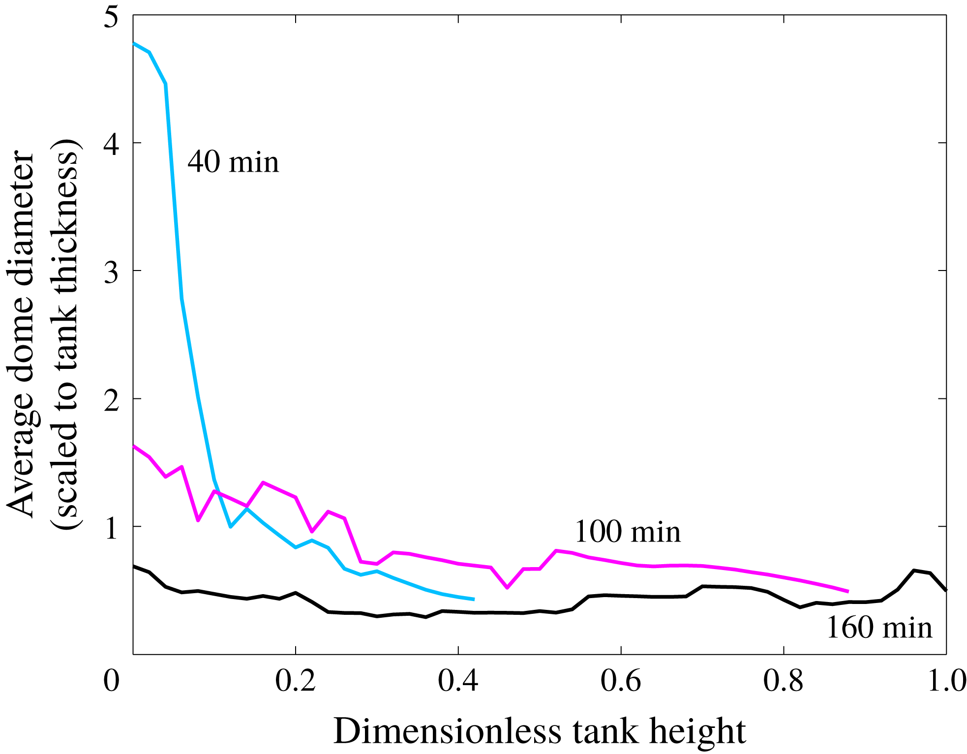
Figure 11. Average diameter of domes scaled to the total fluid thickness
 $h$
as a function of height above base at several times in experiment 21 (in the dome regime).
$h$
as a function of height above base at several times in experiment 21 (in the dome regime).
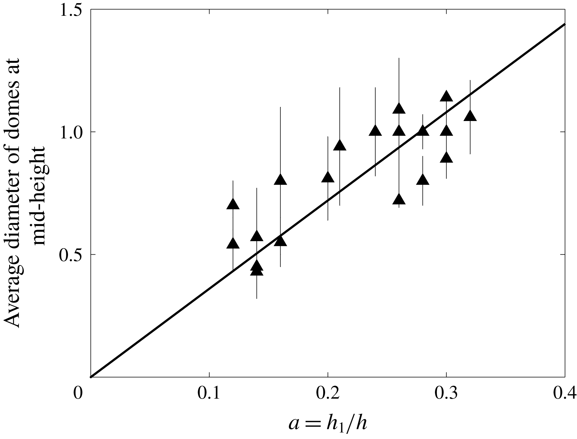
Figure 12. Average dimensionless diameter of domes (scaled to the total reservoir thickness) as a function of dimensionless lower layer thickness (equivalent to the volume fraction of lower fluid in the tank). Data are from all experiments in the dome regime.
Fits to the gamma distribution are shown with dashed lines in figure 10 for the dome regime. The distribution is again close to ‘normal’ at
 $t=0~\text{min}$
(
$t=0~\text{min}$
(
 $k=100$
), but it cannot be fit very well by gamma distributions as the domes grow. Correlation coefficients are smaller than for the stratified regime (
$k=100$
), but it cannot be fit very well by gamma distributions as the domes grow. Correlation coefficients are smaller than for the stratified regime (
 $R\sim 0.98$
), but still acceptable in principle. At late times, however, the distribution is clearly close to ‘uniform’ (with
$R\sim 0.98$
), but still acceptable in principle. At late times, however, the distribution is clearly close to ‘uniform’ (with
 $R>0.99$
at
$R>0.99$
at
 $t=160~\text{min}$
, figure 10). This contrasts with the stratified regime, for which the height distribution is never close to uniform, as shown by low values of the correlation coefficient (
$t=160~\text{min}$
, figure 10). This contrasts with the stratified regime, for which the height distribution is never close to uniform, as shown by low values of the correlation coefficient (
 $R<0.8$
).
$R<0.8$
).
5.3 Regime diagram
Some experiments are such that convection starts in the stratified regime and then shifts to the dome regime due to mixing, and they are lumped together with those that are in the dome regime at all times. Depending on the regime, the CDF varies with time in very different ways and tends towards two very different functions. The goodness of fit to a uniform distribution is excellent in the dome regime and poor in the stratified one, as shown above, which provides an unambiguous discrimination criterion. All else being equal, the buoyancy ratio must be larger than some threshold value to maintain a stratified regime over the whole duration of an experiment.
We found no measurable impact of the viscosity contrast on the boundary between the two regimes, showing that the buoyancy number is the deciding control variable. Figure 13 summarizes observations from all experiments in (
 $B$
,
$B$
,
 $Ra_{H}$
) space. The buoyancy number is calculated using either the conduction scale
$Ra_{H}$
) space. The buoyancy number is calculated using either the conduction scale
 $\unicode[STIX]{x0394}T$
from (2.15) (figure 13
a), corresponding to a value of the buoyancy number noted
$\unicode[STIX]{x0394}T$
from (2.15) (figure 13
a), corresponding to a value of the buoyancy number noted
 $B_{cond}$
, or the maximum temperature difference that develops between the two fluids in the course of an experiment, noted
$B_{cond}$
, or the maximum temperature difference that develops between the two fluids in the course of an experiment, noted
 $T_{12\,max}$
(see § 6), corresponding to a value noted
$T_{12\,max}$
(see § 6), corresponding to a value noted
 $B_{eff}$
(figure 13
b). We discuss later the choice of this temperature difference, which scales with
$B_{eff}$
(figure 13
b). We discuss later the choice of this temperature difference, which scales with
 $\unicode[STIX]{x0394}T\,Ra_{H}^{-1/4}$
(see § 6.3).
$\unicode[STIX]{x0394}T\,Ra_{H}^{-1/4}$
(see § 6.3).
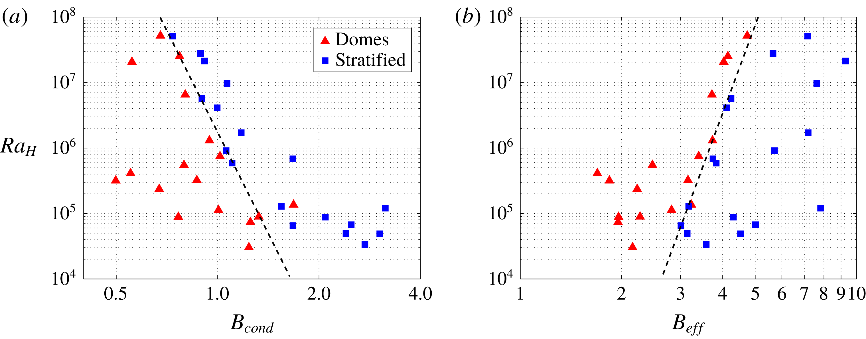
Figure 13. Regime diagrams in (
 $Ra_{H},B$
) space. The buoyancy number
$Ra_{H},B$
) space. The buoyancy number
 $B$
is calculated with the conduction temperature scale
$B$
is calculated with the conduction temperature scale
 $\unicode[STIX]{x0394}T$
from (2.15) in (a) and with the measured temperature difference
$\unicode[STIX]{x0394}T$
from (2.15) in (a) and with the measured temperature difference
 $T_{12\,max}$
in (b), corresponding to two different values of the buoyancy number noted
$T_{12\,max}$
in (b), corresponding to two different values of the buoyancy number noted
 $B_{cond}$
and
$B_{cond}$
and
 $B_{eff}$
respectively. Triangles and squares stand for experiments in the dome and stratified regimes, respectively. Note that one experiment in the dome regime lies in the stratified domain for
$B_{eff}$
respectively. Triangles and squares stand for experiments in the dome and stratified regimes, respectively. Note that one experiment in the dome regime lies in the stratified domain for
 $B=B_{cond}$
and that it is shifted to the boundary between the two regimes for
$B=B_{cond}$
and that it is shifted to the boundary between the two regimes for
 $B=B_{eff}$
.
$B=B_{eff}$
.
The threshold
 $B$
value that separates the two regimes varies by a factor of only 2 over the large range of bulk Rayleigh–Roberts numbers that has been investigated (figure 13). We show results for the two different definitions of the buoyancy number for the sake of discussion, but do not expect that the
$B$
value that separates the two regimes varies by a factor of only 2 over the large range of bulk Rayleigh–Roberts numbers that has been investigated (figure 13). We show results for the two different definitions of the buoyancy number for the sake of discussion, but do not expect that the
 $B_{cond}$
value is appropriate since it relies on a static configuration and temperature distribution. When the
$B_{cond}$
value is appropriate since it relies on a static configuration and temperature distribution. When the
 $B_{cond}$
value is used, two features of the regime diagram are not satisfactory (figure 13
a): one of the dome experiments (experiment 15) shows up in the stratified domain and the threshold buoyancy number for a stratified regime decreases with increasing Rayleigh–Roberts number. One expects instead that it takes increasingly large intrinsic density contrasts to stabilize the lower layer as convection becomes increasingly powerful. With the
$B_{cond}$
value is used, two features of the regime diagram are not satisfactory (figure 13
a): one of the dome experiments (experiment 15) shows up in the stratified domain and the threshold buoyancy number for a stratified regime decreases with increasing Rayleigh–Roberts number. One expects instead that it takes increasingly large intrinsic density contrasts to stabilize the lower layer as convection becomes increasingly powerful. With the
 $B_{eff}$
values, these anomalies disappear (figure 13
b). In this case, the boundary between the two regimes is characterized by
$B_{eff}$
values, these anomalies disappear (figure 13
b). In this case, the boundary between the two regimes is characterized by
 $B_{eff}$
values in a 3–5 range.
$B_{eff}$
values in a 3–5 range.
In experiments with two fluids layers in a Rayleigh–Bénard set-up, with fixed temperatures at the top and bottom of the tank, Davaille et al. (Reference Davaille, Le Bars and Carbonne2003) observed regimes that are similar to the present ones. They used the total temperature difference across the reservoir, which is fixed, to calculate
 $B$
values and obtained threshold values of
$B$
values and obtained threshold values of
 ${\approx}$
0.6. Their result cannot be compared directly with the present ones, in part because we are using the volume-averaged temperatures of the two fluids and in part because temperatures are continuously changing during an experiment. Using volume-averaged temperatures, the threshold
${\approx}$
0.6. Their result cannot be compared directly with the present ones, in part because we are using the volume-averaged temperatures of the two fluids and in part because temperatures are continuously changing during an experiment. Using volume-averaged temperatures, the threshold
 $B$
value for the Rayleigh–Bénard set-up of Davaille et al. (Reference Davaille, Le Bars and Carbonne2003) would hover around a value of approximately 1.2.
$B$
value for the Rayleigh–Bénard set-up of Davaille et al. (Reference Davaille, Le Bars and Carbonne2003) would hover around a value of approximately 1.2.
6 Time changes of thermal structure and the progression of mixing
6.1 Temperature, velocity and compositional fields
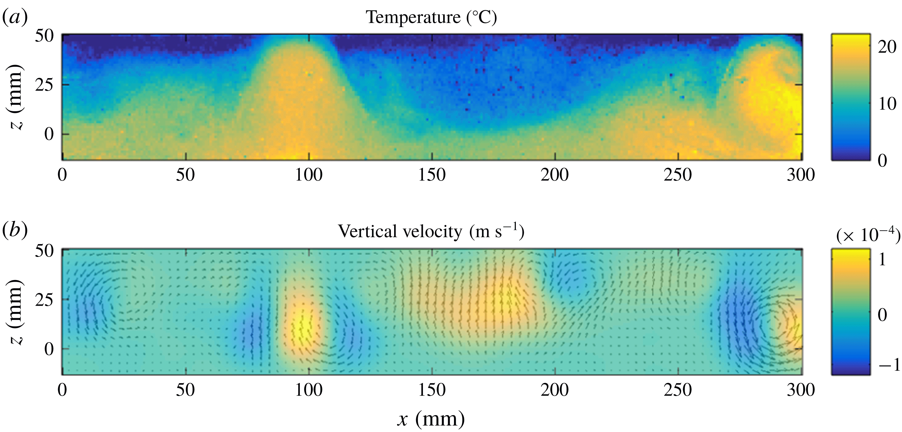
Figure 14. Distributions of temperature (a) and vertical velocity (b) in a vertical cross-section at a position of 100 mm from the front wall and at time
 $=$
60 min in experiment 4 in the ‘dome’ regime.
$=$
60 min in experiment 4 in the ‘dome’ regime.
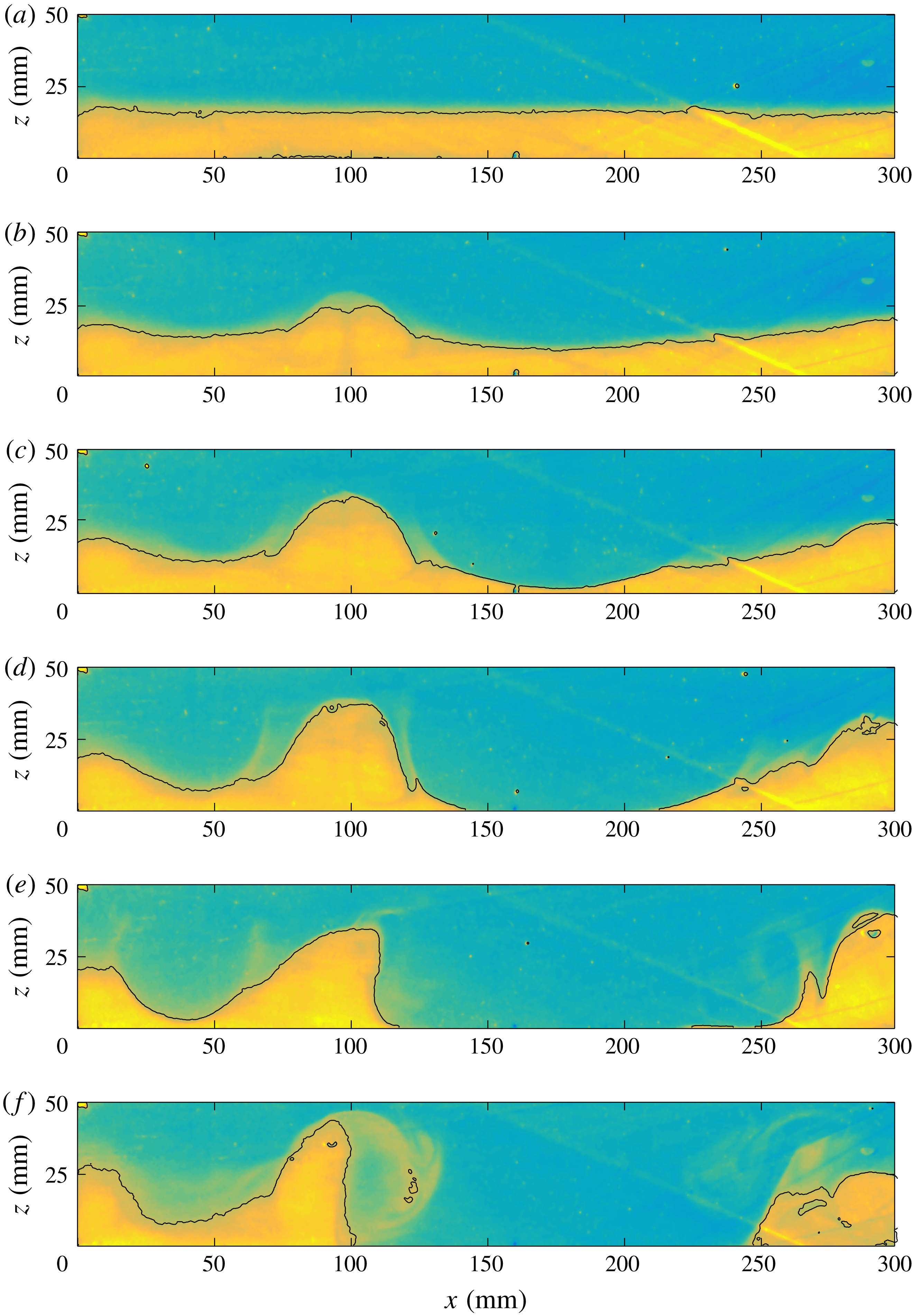
Figure 15. Mixing in the dome regime (experiment 4) at a position of 100 mm from the front wall and time
 $=0$
min (a), 25 min (b), 40 min (c), 55 min (d), 70 min (e), 85 min (f). Black contours correspond to a given pixel intensity value threshold and delineate the boundary between the two fluids as described in § 5. The large dome on the left develops an overhang on its right-hand side. Note the thin upwellings that emanate from the interface and that are made of diluted lower fluid.
$=0$
min (a), 25 min (b), 40 min (c), 55 min (d), 70 min (e), 85 min (f). Black contours correspond to a given pixel intensity value threshold and delineate the boundary between the two fluids as described in § 5. The large dome on the left develops an overhang on its right-hand side. Note the thin upwellings that emanate from the interface and that are made of diluted lower fluid.
Figure 14 illustrates the relationship between the flow structure and the temperature field in the dome regime. The hottest regions are all made of lower fluid, where heat production is larger than average, and it would be difficult to distinguish this overall pattern from that of a Rayleigh–Bénard set-up with the same initial layering arrangement. In this particular case, two large domes have almost reached the top of the tank, where fluid is exposed to the cold boundary, and yet they do not recede. The vertical velocity distribution shows that they develop an internal circulation with a central upwelling surrounded by downwellings. The sharpest velocity gradients occur at their edges and are responsible for the tearing out of lower fluid into the upper one. Both the internal circulation inside the domes and filament entrainment of the lower layer are visible in figure 15. The most interesting feature of this form of convection is that the domes remain stable for long time intervals. Occasionally, the domes fall back down and fold over, encapsulating small blobs of denser upper fluid (figure 15 e,f). In this regime, mixing proceeds through the two different mechanisms that have been described above, but each one is active in one fluid only. The lower fluid entrains upper fluid through folding and encapsulating, whereas the upper fluid tears thin slivers out of lower fluid. For geochemical applications, it is important to note that the lower fluid maintains a well-defined interface with the upper fluid even when it gets diluted to some extent.
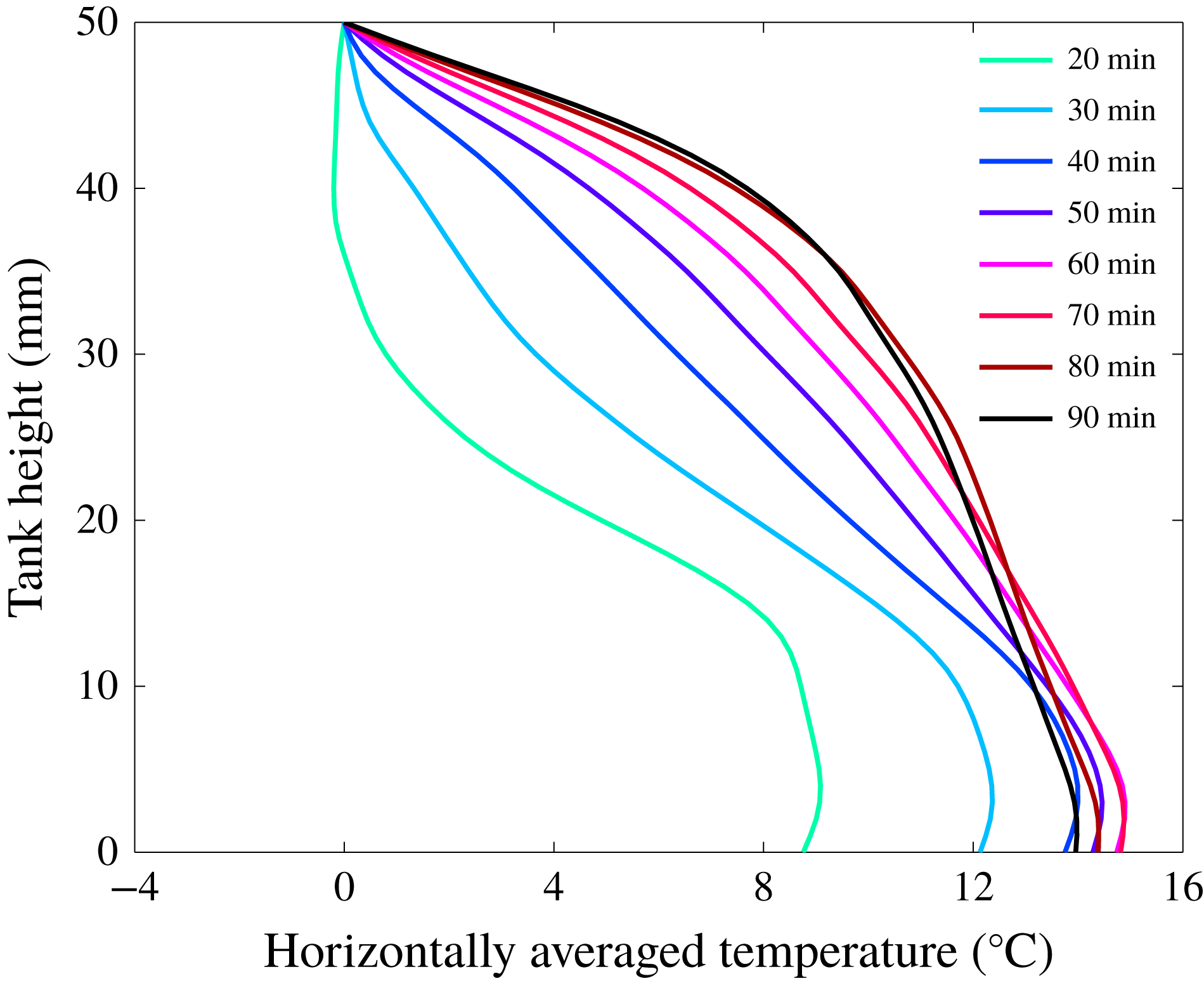
Figure 16. Averaged vertical temperature profiles at different times during experiment 4, which is the same experiment as in figure 14. Colours indicate time evolution from green to blue, red and black. The presence of a warmer lower layer (
 $h_{1}=15~\text{mm}$
) is clearly visible in early stages.
$h_{1}=15~\text{mm}$
) is clearly visible in early stages.
Vertical profiles of the horizontally averaged temperature illustrate the thermal evolution of the two fluids and its relation to the bulk thermal structure. Early profiles are consistent with the presence of two well-separated layers, with the lower one heating up more rapidly than the upper one due to its larger heat production (figure 16). A temperature gradient develops over a large fluid thickness above the initial position of the lower layer, due to the large interface deformation. Without information on the initial structure of the tank, this could be interpreted as due to an unstable thermal boundary layer above a heated horizontal boundary. As hot domes of lower fluid rise, they raise temperatures in the upper fluid and eradicate the sharp temperature gradient that marked the presence of a distinctive lower layer. Late temperature profiles are characterized by a single well-developed thermal boundary layer at the top of an interior region. The upper part of this boundary layer barely changes whilst the temperature distribution below keeps evolving.
In the stratified regime, the interface between the two fluids does not deform by large amounts and does not deviate markedly from its initial position (figure 17). Most of the activity is in the upper fluid. In marked contrast to the experiments in the dome regime, vertical temperature profiles preserve a trace of the initial two-layer configuration for long times (figure 18). These profiles also show a gradual decrease of the thickness of the lower layer, which is indicated by a break in the profiles. In this regime, mixing proceeds exclusively by the entrainment of stretched filaments at the top of cusps of the lower fluid (figure 19).
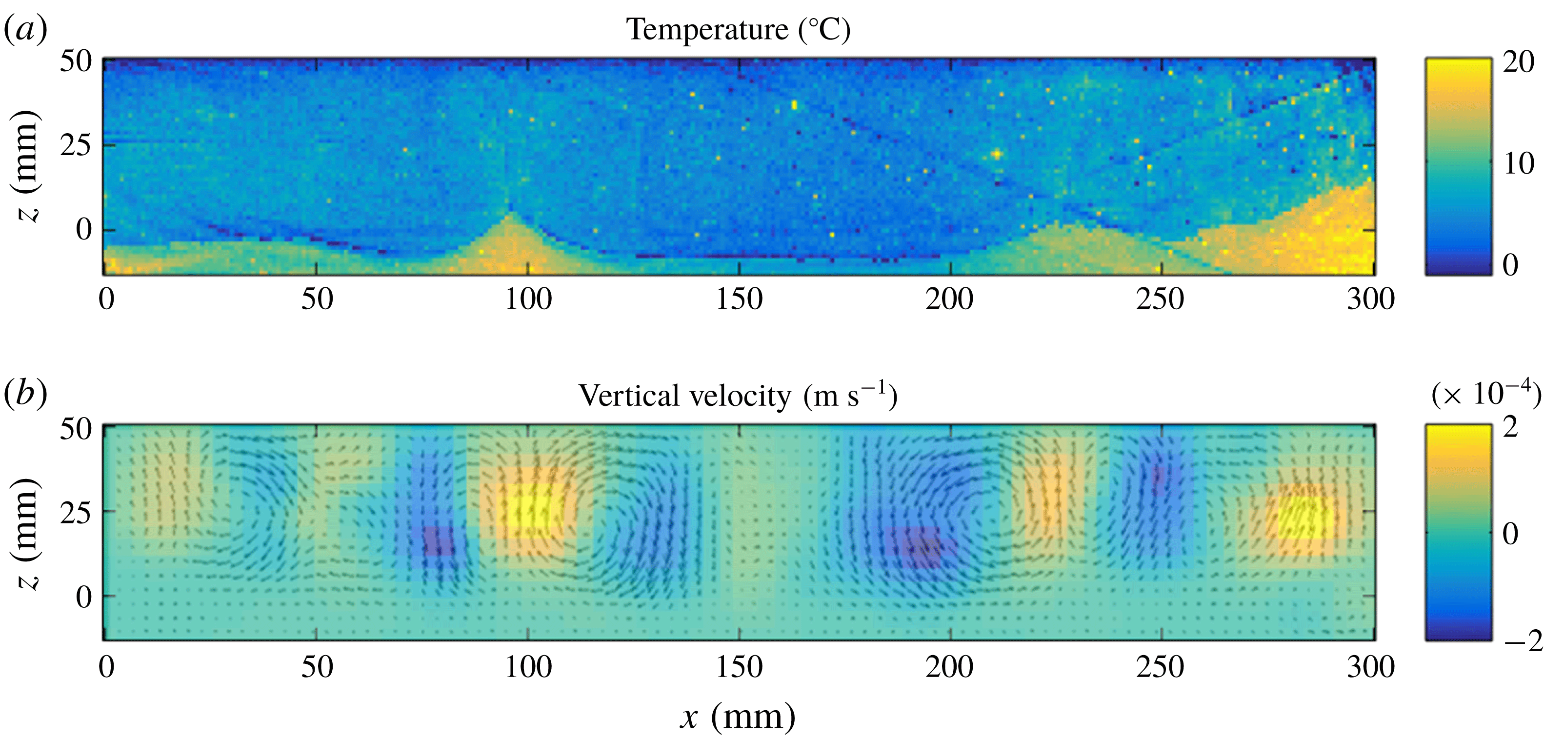
Figure 17. Distributions of temperature (a) and vertical velocity (b) in a vertical cross-section at time
 $=$
90 min in the stratified regime (experiment 7). The lower layer was 12 mm thick initially. This vertical cross-section was obtained at a distance of 100 mm from the front wall.
$=$
90 min in the stratified regime (experiment 7). The lower layer was 12 mm thick initially. This vertical cross-section was obtained at a distance of 100 mm from the front wall.
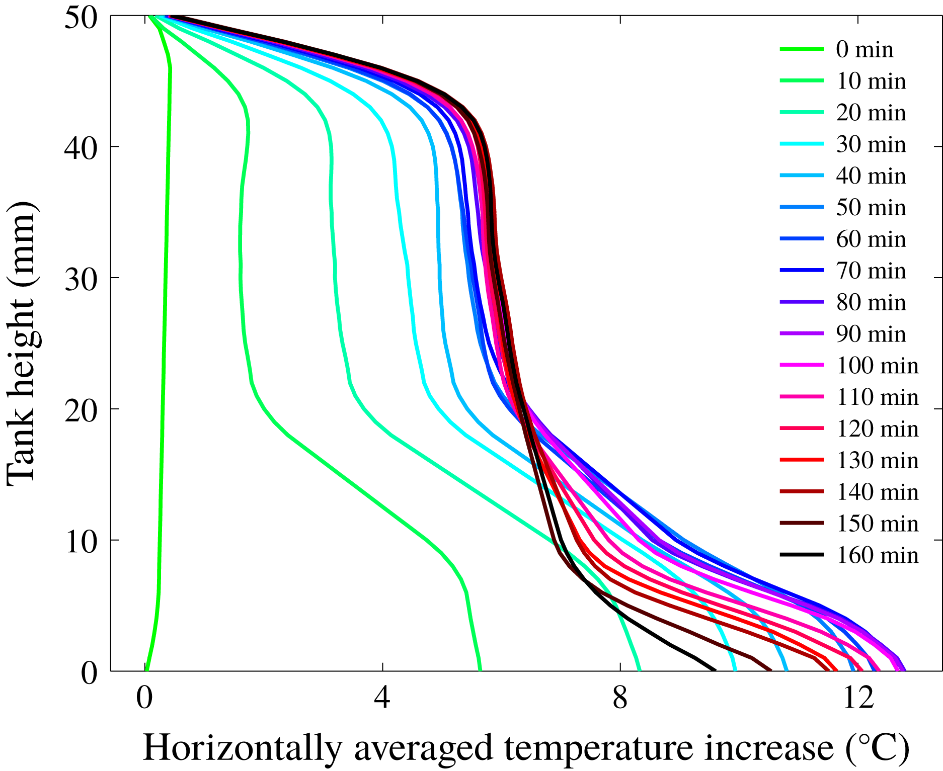
Figure 18. Averaged vertical temperature profiles at different times in the stratified regime (experiment 7). Colours indicate time evolution from green to blue, red and black. Temperatures remain high in a thin region at the base of the tank. Note that, at late times, the temperature profile barely changes in the upper part of the tank whilst the interior structure still evolves at a significant rate.
Figure 19. Entrainment in the stratified regime (experiment 7) at time
 $=$
0 min (a), 70 min (b), 90 min (c), 110 min (d), 130 min (e), 150 min (f). The interface deforms in a number of cusps separated by large basins in the lower fluid. Thin plumes rise from these cusps. This vertical cross-section was obtained at a distance of 100 mm from the front wall.
$=$
0 min (a), 70 min (b), 90 min (c), 110 min (d), 130 min (e), 150 min (f). The interface deforms in a number of cusps separated by large basins in the lower fluid. Thin plumes rise from these cusps. This vertical cross-section was obtained at a distance of 100 mm from the front wall.
6.2 The progression of mixing between the two fluids
We have found that the thermal structure evolves on a different time scale than that of mixing. As discussed above, all experiments end up with a steady-state thermal structure that is identical to that for a homogeneous reservoir. As discussed above, this does not imply that the two fluids are truly mixed in the chemical sense, such that there are no variations of composition at a local scale. In order to determine how mixing progresses, we have focussed on the lower fluid and measured two different variables. One is the volume of lower fluid that is separated from the upper fluid by a well-defined interface, as discussed above, and the other is the area occupied by lower fluid at the base of the tank. The latter allows us to track the gradual disappearance of a lower layer independently of volume changes, which is appropriate for the Earth because the starting volume of primordial material at the base of the mantle is ill constrained.
Figure 20. Dome regime: evolution in time of the lower layer volume scaled by its initial value
 $V_{0}$
(a), of the occupied area at the lower boundary scaled by its initial value
$V_{0}$
(a), of the occupied area at the lower boundary scaled by its initial value
 $A_{0}$
(b), of the volume average temperature of the lower layer
$A_{0}$
(b), of the volume average temperature of the lower layer
 $T_{1}$
(c), of the top layer
$T_{1}$
(c), of the top layer
 $T_{2}$
(d), volume-average temperature contrast between the two layers
$T_{2}$
(d), volume-average temperature contrast between the two layers
 $T_{12}$
(e) and of the whole volume
$T_{12}$
(e) and of the whole volume
 $\langle T\rangle$
(f) for experiment 21;
$\langle T\rangle$
(f) for experiment 21;
 $t_{0}$
is the time corresponding to the onset of mixing and
$t_{0}$
is the time corresponding to the onset of mixing and
 $t_{end}$
marks the end of the well-defined lower fluid reservoir.
$t_{end}$
marks the end of the well-defined lower fluid reservoir.
The volume and area of lower fluid decrease continuously during an experiment (figure 20
a,b). Mixing/mingling does not begin at time
 $t=0$
when the first scans are carried out after the microwave emitter is switched on, because it takes a finite temperature difference across the layers to initiate convection. Thus, changes of volume or area of lower fluid become measurable after some time. Mixing/mingling may be considered complete when the lower fluid has been completely swept away from the base of the tank, corresponding to a zero area, and when the volume that is contained in individual parcels, or a deformed layer at the base of the tank, drops below detection level. Defining departure from an initial value or a hit at a target final value requires rather arbitrary thresholds and depends on measurement accuracy as well as on the time interval between two frames. We chose instead to use data in the intermediate range because these focus on the times when mixing is most active, as opposed to early and late phases when the data are either ramping up or winding down. These data are close to a linear trend, indicating that the mixing rate does not vary by large factors in the course of an experiment. Variations of the mixing rate are due to long-period fluctuations of the interior structure, due for example to the rise and fall cycle of lower fluid domes when they exist. We extrapolate the trends in the volume and area data to zero, which provides an estimate of the mixing time, noted
$t=0$
when the first scans are carried out after the microwave emitter is switched on, because it takes a finite temperature difference across the layers to initiate convection. Thus, changes of volume or area of lower fluid become measurable after some time. Mixing/mingling may be considered complete when the lower fluid has been completely swept away from the base of the tank, corresponding to a zero area, and when the volume that is contained in individual parcels, or a deformed layer at the base of the tank, drops below detection level. Defining departure from an initial value or a hit at a target final value requires rather arbitrary thresholds and depends on measurement accuracy as well as on the time interval between two frames. We chose instead to use data in the intermediate range because these focus on the times when mixing is most active, as opposed to early and late phases when the data are either ramping up or winding down. These data are close to a linear trend, indicating that the mixing rate does not vary by large factors in the course of an experiment. Variations of the mixing rate are due to long-period fluctuations of the interior structure, due for example to the rise and fall cycle of lower fluid domes when they exist. We extrapolate the trends in the volume and area data to zero, which provides an estimate of the mixing time, noted
 $t_{end}$
. As shown below, we found that the volume and area data lead to values of
$t_{end}$
. As shown below, we found that the volume and area data lead to values of
 $t_{end}$
that are nearly identical. The best-fit line also provides an estimate of the time when mixing starts to have a detectable impact on volume and area, noted
$t_{end}$
that are nearly identical. The best-fit line also provides an estimate of the time when mixing starts to have a detectable impact on volume and area, noted
 $t_{o}$
.
$t_{o}$
.
In the dome regime (figure 20), the volume (figure 20
a) and area (figure 20
b) of lower fluid begin to deviate from their initial values and go to zero at about the same times. The onset of mixing at a significant rate is linked to breaks in the time evolutions of the average temperature of the lower fluid
 $T_{1}$
(figure 20
c) and of the temperature difference between the two fluids
$T_{1}$
(figure 20
c) and of the temperature difference between the two fluids
 $T_{12}$
(figure 20
e). Both temperatures peak at approximately the same time as mixing progresses. One should note that, as might be expected, the temperature difference decreases to zero together with the volume and area of lower fluid. Due to mixing, the amount of lower fluid diminishes steadily, which favours thermal equilibrium with the upper fluid.
$T_{12}$
(figure 20
e). Both temperatures peak at approximately the same time as mixing progresses. One should note that, as might be expected, the temperature difference decreases to zero together with the volume and area of lower fluid. Due to mixing, the amount of lower fluid diminishes steadily, which favours thermal equilibrium with the upper fluid.
In the stratified regime (figure 21), there is a marked difference with the dome regime early in an experiment. Mixing is effective before the cusp and basin morphology reaches maximum amplitude. Due to the resilience of the lower layer, the lower fluid sees its volume decrease even though it is spread over the whole base of the reservoir. The area of lower fluid begins to decrease at a larger time but goes to zero at about the same time as the volume. At this time the temperature difference between the two fluids drops to zero rather abruptly because there is no detectable lower fluid present.
6.3 Changes of thermal structure
We have tracked changes of thermal structure as a function of time using four different temperature values: the average temperatures of the upper and lower fluids
 $T_{1}$
and
$T_{1}$
and
 $T_{2}$
, their difference
$T_{2}$
, their difference
 $T_{12}$
and the volume-averaged temperature for the whole tank
$T_{12}$
and the volume-averaged temperature for the whole tank
 $\langle T\rangle$
(figure 20
c–f in the dome regime and figure 21
c–f in the stratified regime). The evolutions of all these temperatures are modulated by low-amplitude long-period oscillations which reflect the changes of thermal structure and mixing rate that occur in the tank.
$\langle T\rangle$
(figure 20
c–f in the dome regime and figure 21
c–f in the stratified regime). The evolutions of all these temperatures are modulated by low-amplitude long-period oscillations which reflect the changes of thermal structure and mixing rate that occur in the tank.
In the dome regime, the average temperature of the lower fluid, whose volume is decreasing with time as mixing progresses, reaches a peak value and then decreases as the ever-shrinking parcels of lower fluid equilibrate with the colder surrounding fluid. As the upper fluid ingests lower fluid, it gradually warms up, but sensible heat plays a minor role: the slow rate of warming is due to the enhanced heat production. The progression of mixing is illustrated clearly by a decreasing thermal contrast between the two fluids. In this regime, mixing is effected by the two different processes that have already been described. Both act to decrease the thermal contrast between the two fluids in two opposite ways, the former (filament entrainment) by enhancing heat production in the upper fluid and the latter (folding of lower layer) by lessening heat production in the lower fluid. We found that the latter is consistently much less effective than the former.
Figure 21. Stratified regime: time evolution of the lower layer volume scaled by its initial value
 $V_{0}$
(a), of the occupied area at the lower boundary scaled by its initial value
$V_{0}$
(a), of the occupied area at the lower boundary scaled by its initial value
 $A_{0}$
(b), of the volume average temperature of the lower layer
$A_{0}$
(b), of the volume average temperature of the lower layer
 $T_{1}$
(c), of the top layer
$T_{1}$
(c), of the top layer
 $T_{2}$
(d), volume-average temperature contrast between the two layers
$T_{2}$
(d), volume-average temperature contrast between the two layers
 $T_{12}$
(e) and of the whole volume
$T_{12}$
(e) and of the whole volume
 $\langle T\rangle$
(f) for experiment 34;
$\langle T\rangle$
(f) for experiment 34;
 $t_{0}$
(vol, area) marks the time when mixing has a measurable effect on the volume and area, respectively, and
$t_{0}$
(vol, area) marks the time when mixing has a measurable effect on the volume and area, respectively, and
 $t_{end}$
marks the disappearance of a well-defined lower fluid reservoir.
$t_{end}$
marks the disappearance of a well-defined lower fluid reservoir.
Figure 22. Volume-average temperature contrast between the two layers
 $T_{12\,max}/\unicode[STIX]{x0394}T$
(circles) as a function of the Rayleigh–Roberts number. The line represents a power-law best fit with the exponent fixed at
$T_{12\,max}/\unicode[STIX]{x0394}T$
(circles) as a function of the Rayleigh–Roberts number. The line represents a power-law best fit with the exponent fixed at
 $-1/4$
and calculated with data for
$-1/4$
and calculated with data for
 $Ra_{H}>10^{5}$
(see also table 5).
$Ra_{H}>10^{5}$
(see also table 5).
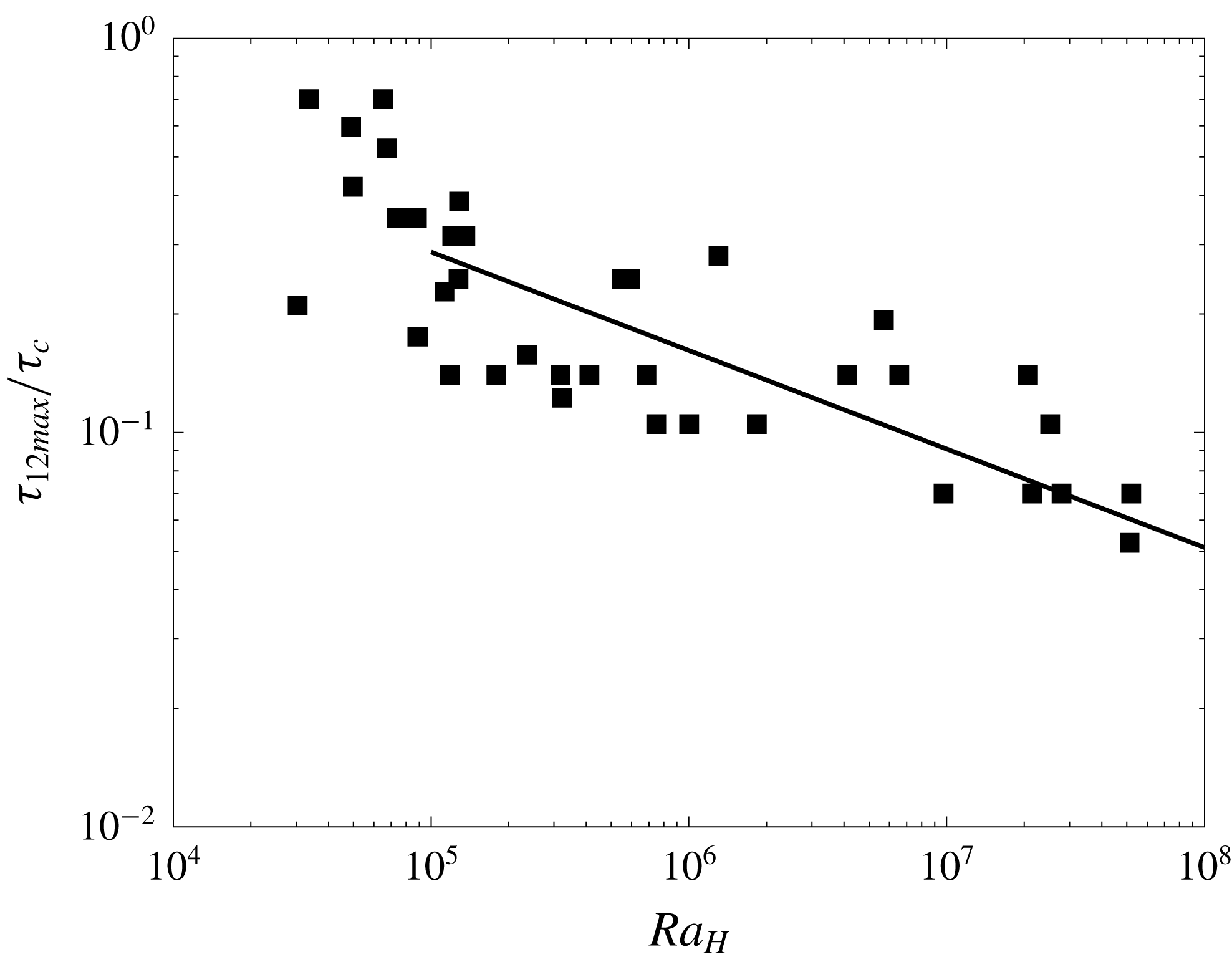
Figure 23. Dependence of the time scale
 $\unicode[STIX]{x1D70F}_{12\,max}/\unicode[STIX]{x1D70F}_{c}$
of the volume-average temperature contrast on the Rayleigh–Roberts number. The line corresponds to a power-law fit with an exponent fixed at
$\unicode[STIX]{x1D70F}_{12\,max}/\unicode[STIX]{x1D70F}_{c}$
of the volume-average temperature contrast on the Rayleigh–Roberts number. The line corresponds to a power-law fit with an exponent fixed at
 $-1/4$
(table 5).
$-1/4$
(table 5).
The temperature difference between the two layers, noted
 $T_{12}$
, peaks at some specific time in both regimes. The time of the thermal peak marks a change in the impact of mixing on the system, such that the influence of the lower fluid on the bulk thermal structure begins to wane. We have determined the magnitude of the peak temperature difference
$T_{12}$
, peaks at some specific time in both regimes. The time of the thermal peak marks a change in the impact of mixing on the system, such that the influence of the lower fluid on the bulk thermal structure begins to wane. We have determined the magnitude of the peak temperature difference
 $T_{12}$
, noted
$T_{12}$
, noted
 $T_{12\,max}$
, and the time at which it occurs, noted
$T_{12\,max}$
, and the time at which it occurs, noted
 $\unicode[STIX]{x1D70F}_{12\,max}$
(table 2). The magnitude of the peak is well constrained but the time is not due to two factors. The peak may be quite flat and spread over a finite time interval in some cases. In addition, measurements are repeated at time intervals of 5 min because of the large number of scans that are made, which makes for a poor time resolution. For our present purposes, we do not need accurate determinations of the peak time and the experimental procedure was the result of a compromise between measurement repetition and data coverage. We have scaled
$\unicode[STIX]{x1D70F}_{12\,max}$
(table 2). The magnitude of the peak is well constrained but the time is not due to two factors. The peak may be quite flat and spread over a finite time interval in some cases. In addition, measurements are repeated at time intervals of 5 min because of the large number of scans that are made, which makes for a poor time resolution. For our present purposes, we do not need accurate determinations of the peak time and the experimental procedure was the result of a compromise between measurement repetition and data coverage. We have scaled
 $T_{12\,max}$
and
$T_{12\,max}$
and
 $\unicode[STIX]{x1D70F}_{12\,max}$
values to the reference conduction temperature difference
$\unicode[STIX]{x1D70F}_{12\,max}$
values to the reference conduction temperature difference
 $\unicode[STIX]{x0394}T$
and time scale
$\unicode[STIX]{x0394}T$
and time scale
 $\unicode[STIX]{x1D70F}_{c}$
(figures 22 and 23). The data are consistent with power-law relationships with the bulk Rayleigh–Roberts number
$\unicode[STIX]{x1D70F}_{c}$
(figures 22 and 23). The data are consistent with power-law relationships with the bulk Rayleigh–Roberts number
 $Ra_{H}$
and we have determined the corresponding coefficients using a best-fit procedure. The best-fit exponents are remarkably close to values for internally heated homogeneous layers (table 5).
$Ra_{H}$
and we have determined the corresponding coefficients using a best-fit procedure. The best-fit exponents are remarkably close to values for internally heated homogeneous layers (table 5).
The peak time data in figure 23 obviously do not provide strong evidence for a power-law relationship but what concerns us here is a comparison between this time and the thermal relaxation time for the reservoir,
 $\unicode[STIX]{x1D70F}_{e}$
(
$\unicode[STIX]{x1D70F}_{e}$
(
 $\unicode[STIX]{x1D70F}_{12\,max}\approx 5.1\,Ra_{H}^{-1/4}$
whereas
$\unicode[STIX]{x1D70F}_{12\,max}\approx 5.1\,Ra_{H}^{-1/4}$
whereas
 $\unicode[STIX]{x1D70F}_{e}=3.0\,Ra_{H}^{-1/4}$
). Thus, at the time of the peak thermal contrast,
$\unicode[STIX]{x1D70F}_{e}=3.0\,Ra_{H}^{-1/4}$
). Thus, at the time of the peak thermal contrast,
 $\langle T\rangle$
is within 18 % of its final value and the bulk thermal structure of the reservoir is close to the final steady state, but mixing is far from completion. At that time, for example, the volume of lower fluid at the base of the tank is approximately 70 % of its initial value in the dome regime and has barely changed in the stratified regime (figures 20 and 21). This shows that thermal steady state is achieved long before complete mingling or mixing.
$\langle T\rangle$
is within 18 % of its final value and the bulk thermal structure of the reservoir is close to the final steady state, but mixing is far from completion. At that time, for example, the volume of lower fluid at the base of the tank is approximately 70 % of its initial value in the dome regime and has barely changed in the stratified regime (figures 20 and 21). This shows that thermal steady state is achieved long before complete mingling or mixing.
Table 5. Parameters of empirical best-fit power laws for the volume-average temperature difference between the two layers
 $T_{12\,max}$
and the time at which this maximum occurs
$T_{12\,max}$
and the time at which this maximum occurs
 $\unicode[STIX]{x1D70F}_{12\,max}$
at high values of the Rayleigh–Roberts number (
$\unicode[STIX]{x1D70F}_{12\,max}$
at high values of the Rayleigh–Roberts number (
 $Ra_{H}\geqslant 10^{5}$
).
$Ra_{H}\geqslant 10^{5}$
).
We are interested in the large-scale flow pattern and mixing processes, which are intimately linked to one another and which are driven by thermally induced density differences. The peak temperature contrast between the two layers, noted
 $T_{12\,max}$
, is associated with the active mixing phase and is therefore appropriate for calculating the buoyancy number. This buoyancy number, noted
$T_{12\,max}$
, is associated with the active mixing phase and is therefore appropriate for calculating the buoyancy number. This buoyancy number, noted
 $B_{eff}$
, is used in the regime diagram of figure 13(b).
$B_{eff}$
, is used in the regime diagram of figure 13(b).
6.4 Mixing time
Mixing proceeds mostly by the entrainment of thin slivers of one fluid into the other, which occurs at the interface between the two fluids. Thus, we can apply the same reasoning as Davaille (Reference Davaille1999b ), who derived a relationship for the entrainment rate of a denser layer based on scalings for the shear stress that is imparted on the interface between two convecting fluid layers:
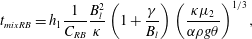 $$\begin{eqnarray}\displaystyle t_{mix\,RB}=h_{1}{\displaystyle \frac{1}{C_{RB}}}{\displaystyle \frac{B_{l}^{2}}{\unicode[STIX]{x1D705}}}\left(1+{\displaystyle \frac{\unicode[STIX]{x1D6FE}}{B_{l}}}\right)\left({\displaystyle \frac{\unicode[STIX]{x1D705}\unicode[STIX]{x1D707}_{2}}{\unicode[STIX]{x1D6FC}\unicode[STIX]{x1D70C}g\unicode[STIX]{x1D703}}}\right)^{1/3}, & & \displaystyle\end{eqnarray}$$
where
 $C_{RB}$
is a proportionality constant and
$C_{RB}$
is a proportionality constant and
 $B_{l}$
is a buoyancy factor related to the temperature difference between the two layers
$B_{l}$
is a buoyancy factor related to the temperature difference between the two layers
 $\unicode[STIX]{x1D703}$
(
$\unicode[STIX]{x1D703}$
(
 $B_{l}=\unicode[STIX]{x0394}\unicode[STIX]{x1D70C}/\unicode[STIX]{x1D6FC}\unicode[STIX]{x1D70C}\unicode[STIX]{x1D703}$
). The (
$B_{l}=\unicode[STIX]{x0394}\unicode[STIX]{x1D70C}/\unicode[STIX]{x1D6FC}\unicode[STIX]{x1D70C}\unicode[STIX]{x1D703}$
). The (
 $1+\unicode[STIX]{x1D6FE}/B_{l}$
) was added to account for the viscosity contrast effect in the experiments. The volume of lower fluid is small compared to that of the upper fluid, implying that mixing does not affect significantly the physical properties of the upper fluid. This is why Davaille (Reference Davaille1999b
) used the physical properties of the upper fluid.
$1+\unicode[STIX]{x1D6FE}/B_{l}$
) was added to account for the viscosity contrast effect in the experiments. The volume of lower fluid is small compared to that of the upper fluid, implying that mixing does not affect significantly the physical properties of the upper fluid. This is why Davaille (Reference Davaille1999b
) used the physical properties of the upper fluid.
Davaille (Reference Davaille1999a
) scaled the temperature difference between the layers
 $\unicode[STIX]{x1D703}$
to the thermal contrast across the tank, which remains constant in the Rayleigh–Bénard configuration of her experiments and determined a best-fit experimental coefficient
$\unicode[STIX]{x1D703}$
to the thermal contrast across the tank, which remains constant in the Rayleigh–Bénard configuration of her experiments and determined a best-fit experimental coefficient
 $C_{RB}=0.61\pm 0.05$
. We cannot follow the same line of reasoning because the total thermal contrast evolves with time and eventually settles to zero, which is only relevant for the final homogenized fluid. Following Fourel et al. (Reference Fourel, Limare, Jaupart, Surducan, Farnetani, Kaminski, Neamtu and Surducan2017) we use again the maximum temperature difference between the two fluids:
$C_{RB}=0.61\pm 0.05$
. We cannot follow the same line of reasoning because the total thermal contrast evolves with time and eventually settles to zero, which is only relevant for the final homogenized fluid. Following Fourel et al. (Reference Fourel, Limare, Jaupart, Surducan, Farnetani, Kaminski, Neamtu and Surducan2017) we use again the maximum temperature difference between the two fluids:
 $$\begin{eqnarray}\displaystyle t_{mix\,IH}=h_{1}{\displaystyle \frac{1}{C_{IH}}}{\displaystyle \frac{B_{eff}^{2}}{\unicode[STIX]{x1D705}}}\left(1+{\displaystyle \frac{\unicode[STIX]{x1D6FE}}{B_{eff}}}\right)\left({\displaystyle \frac{\unicode[STIX]{x1D705}\unicode[STIX]{x1D707}_{2}}{\unicode[STIX]{x1D6FC}\unicode[STIX]{x1D70C}gT_{12\,max}}}\right)^{1/3}. & & \displaystyle\end{eqnarray}$$
The results are shown in figure 24. This scaling holds remarkably well over 2 orders of magnitude with an experimental constant of
 $C_{IH}=0.08\pm 0.01$
. The data exhibit some scatter around the best-fit relationship but this scatter is related neither to the convection regime (i.e. dome or stratified) nor to the viscosity contrast (
$C_{IH}=0.08\pm 0.01$
. The data exhibit some scatter around the best-fit relationship but this scatter is related neither to the convection regime (i.e. dome or stratified) nor to the viscosity contrast (
 $\unicode[STIX]{x1D6FE}$
value).
$\unicode[STIX]{x1D6FE}$
value).
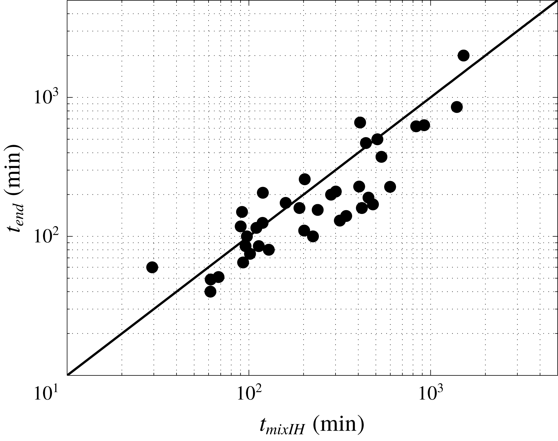
Figure 24. Experimental versus theoretical mixing time in internally heated convection experiments:
 $t_{experimental}$
is equal to
$t_{experimental}$
is equal to
 $t_{end}$
, which is deduced from both the volume and area data at the lower boundary;
$t_{end}$
, which is deduced from both the volume and area data at the lower boundary;
 $t_{mix\,IH}$
is calculated from (6.2) with an experimental constant
$t_{mix\,IH}$
is calculated from (6.2) with an experimental constant
 $C_{IH}=0.08$
.
$C_{IH}=0.08$
.
Two asymptotic expressions for the mixing time shed light on the viscosity control of mixing phenomena. If
 $\unicode[STIX]{x1D6FE}\gg 1$
:
$\unicode[STIX]{x1D6FE}\gg 1$
:
 $$\begin{eqnarray}\displaystyle t_{mix\,IH}\sim \unicode[STIX]{x1D6FE}T_{12\,max}^{-(4/3)}. & & \displaystyle\end{eqnarray}$$
If
 $\unicode[STIX]{x1D6FE}\ll 1$
, the mixing time does not depend on the viscosity of the lower fluid:
$\unicode[STIX]{x1D6FE}\ll 1$
, the mixing time does not depend on the viscosity of the lower fluid:
 $$\begin{eqnarray}\displaystyle t_{mix\,IH}\sim T_{12\,max}^{-(7/3)}. & & \displaystyle\end{eqnarray}$$
7 Discussion
7.1 Internal versus basal heating
In a homogeneous fluid layer, internal heating breaks the symmetry between top and bottom that exists in a Rayleigh–Bénard configuration, where heat is supplied through the base of the tank and extracted at the top. In the latter, convection can be described as sets of equally strong upwellings and downwellings issuing from thermal boundary layers at the top and bottom. In the internal heating configuration, there is only one unstable boundary layer at the top of the reservoir, implying that convection proceeds by strong cold downwellings and a diffuse upward return flow with weak thermal anomalies (Vilella et al. Reference Vilella, Limare, Jaupart, Farnetani, Fourel and Kaminski2018). Adding a denser basal layer with higher than average heat production could be considered as akin to basal heating for the upper fluid, but this may be misleading. In many cases, the large interface deformation that occurs is responsible for vertical temperature variations over a thick region at the base of the tank (figure 3), which could be mistaken for a basal thermal boundary layer due to heating from below. This lower region is such that heat transport is not dominated by conduction and is a transient feature, as shown by figure 3.
Our experiments show that, in a two-layer stratified configuration, internal heating leads to structures and flow patterns that are very similar to those of Rayleigh–Bénard set-ups. In the dome regime, the lower layer gets distorted and split into patches or piles with a range of shapes that are the same in both types of experimental conditions. Basal patches act to localize upwellings and plumes at their edges independently of the mode of heating. One important difference with a Rayleigh–Bénard set-up is that the large protrusions of lower fluid that grow into the upper fluid in the dome regime are remarkably steady and may persist over large fractions of the mixing time. The domes are made of intrinsically denser fluid, but they are heated internally at a larger rate than the upper fluid, which maintains a positive temperature anomaly. They are also supported by stresses imparted by adjacent upwellings in the upper fluid.
7.2 Earth’s mantle heterogeneity
Geochemical and geophysical data indicate that the mantle is heterogeneous, but the origins and locations of the different mantle components remain debated. A major stumbling block is that the initial mantle composition, acquired when the Earth began to behave as an isolated system with no external input, is not known precisely (Jackson & Carlson Reference Jackson and Carlson2012; Gale et al. Reference Gale, Dalton, Langmuir, Su and Schilling2013). In addition, the primordial mantle may well have been stratified. Today, after 4.5 billion years of evolution, the upper mantle is made of different components mixed in variable proportions and two extreme compositions have been determined, called for the sake of convenience ‘enriched’ and ‘depleted’ respectively. Here, ‘enriched’ is only a relative term defined with respect to ‘depleted’ (in other words it does not necessarily imply material that has effectively been enriched with respect to the starting composition). The enriched components are brought by mantle plumes coming from large depths.
Our experiments show that, starting from a two-layer reservoir, the upper fluid becomes a mixture of the two different fluids with no detectable large-scale changes of concentration with depth, save for residual patches of lower fluids at the base which slowly get eroded by plumes. These plumes are made of two components: upper fluid, which has become a mixture of the initial lower and upper fluids, and pure (or weakly diluted) initial lower fluid. Translated into geochemical parlance, these plumes are therefore enriched with respect to the surrounding fluid, but they are not made of a pure primordial end member. At any given time, they are not made with exactly the same proportions of the two components and hence do not have the same composition. This is consistent with the geochemical data (Gale et al. Reference Gale, Dalton, Langmuir, Su and Schilling2013).
This brief overview of geochemical constraints emphasizes the key contribution of mantle plumes, which sample deep mantle material. As the Earth has been undergoing convection for most of its lifetime, one must address two questions. One is whether or not primordial mantle material can survive and avoid being mixed into the bulk mantle for more than four billions years. This depends on many physical properties that are not known precisely, such as the intrinsic density of primordial mantle material. As the mixing time depends mostly on processes at the interface between the two materials and on the temperature difference between them independently of the mode of heating, the present study cannot add much to earlier analyses (Davaille et al.
Reference Davaille, Girard and Le Bars2002). Using available constraints on physical properties and temperature differences in the Earth’s mantle, Davaille et al. (Reference Davaille, Girard and Le Bars2002) have concluded that primordial material can survive for many billions of years at the base of the mantle. Our results lead to the same conclusion if the viscosity and density contrasts are large enough. Figure 25 shows how the amount of enriched material and its volume-averaged temperature evolve with time for parameter values that are representative of mantle conditions:
 $h_{1}=400~\text{km}$
,
$h_{1}=400~\text{km}$
,
 $a=0.13$
, enrichment factor
$a=0.13$
, enrichment factor
 $F=3$
,
$F=3$
,
 $\unicode[STIX]{x1D707}_{2}=10^{21}~\text{Pa}~\text{s}$
, viscosity ratio
$\unicode[STIX]{x1D707}_{2}=10^{21}~\text{Pa}~\text{s}$
, viscosity ratio
 $\unicode[STIX]{x1D6FE}=10$
, intrinsic density contrast
$\unicode[STIX]{x1D6FE}=10$
, intrinsic density contrast
 $\unicode[STIX]{x0394}\unicode[STIX]{x1D70C}/\unicode[STIX]{x1D70C}=1\,\%$
,
$\unicode[STIX]{x0394}\unicode[STIX]{x1D70C}/\unicode[STIX]{x1D70C}=1\,\%$
,
 $Ra_{H}=10^{8}$
and a starting temperature of
$Ra_{H}=10^{8}$
and a starting temperature of
 $1600\,^{\circ }\text{C}$
. With
$1600\,^{\circ }\text{C}$
. With
 $\unicode[STIX]{x1D6FC}=2\times 10^{-5}~\text{K}^{-1}$
, the buoyancy number is
$\unicode[STIX]{x1D6FC}=2\times 10^{-5}~\text{K}^{-1}$
, the buoyancy number is
 $B_{eff}=1.2$
, implying a dome regime. In this example, the key difference with the Rayleigh–Bénard configuration is that the time and temperature scales do not depend on an arbitrarily fixed temperature difference between the top and bottom of the reservoir: they are deduced from the total amount and distribution of heat-producing elements. This calculation is just one in a set of many and is only meant to illustrate the time and temperature scales involved in mantle conditions. It shows a lower fluid temperature that initially rises and peaks after almost a billion years, and a lower fluid volume that has decreased by approximately 40 % after 4.5 billion years. Interestingly, the average temperature difference between the lower and upper fluids stays quite constant at
$B_{eff}=1.2$
, implying a dome regime. In this example, the key difference with the Rayleigh–Bénard configuration is that the time and temperature scales do not depend on an arbitrarily fixed temperature difference between the top and bottom of the reservoir: they are deduced from the total amount and distribution of heat-producing elements. This calculation is just one in a set of many and is only meant to illustrate the time and temperature scales involved in mantle conditions. It shows a lower fluid temperature that initially rises and peaks after almost a billion years, and a lower fluid volume that has decreased by approximately 40 % after 4.5 billion years. Interestingly, the average temperature difference between the lower and upper fluids stays quite constant at
 ${\approx}400\,^{\circ }\text{C}$
for several billion years.
${\approx}400\,^{\circ }\text{C}$
for several billion years.
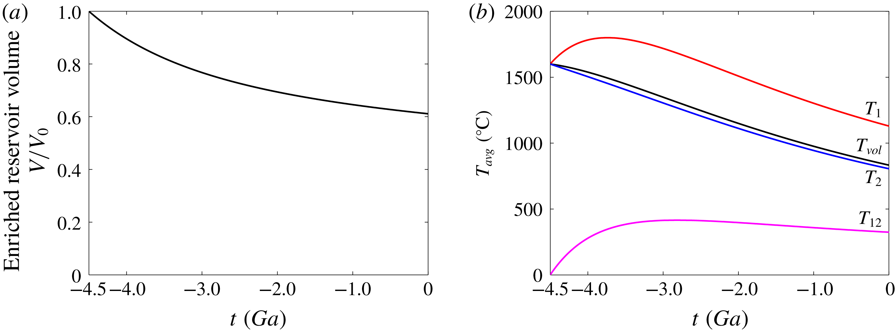
Figure 25. Time variation of the volume (a) and the volume-averaged temperatures (b) of an enriched basal reservoir for
 $h_{1}=400~\text{km}$
,
$h_{1}=400~\text{km}$
,
 $F=3$
,
$F=3$
,
 $Ra_{H}=10^{8}$
,
$Ra_{H}=10^{8}$
,
 $B_{eff}=1.2$
,
$B_{eff}=1.2$
,
 $\unicode[STIX]{x1D6FE}=10$
and
$\unicode[STIX]{x1D6FE}=10$
and
 $\unicode[STIX]{x0394}\unicode[STIX]{x1D70C}/\unicode[STIX]{x1D70C}=1\,\%$
.
$\unicode[STIX]{x0394}\unicode[STIX]{x1D70C}/\unicode[STIX]{x1D70C}=1\,\%$
.
A second question is whether or not a basal heat flux is required to generate deep plumes. This is associated with a subsidiary question: has the basal heat flux always been as strong as today in the past? Heating the mantle from below depends on the cooling of the core, which in turn depends on the secular evolution of the coupled core–mantle system. Thus, the answer to the subsidiary question requires a full thermal model of the Earth, which is outside the scope of this paper. We have shown, however, that deep mantle plumes with the required characteristics can be generated by enriched lower mantle material with no heat coming from the core.
7.3 The cooling of the Earth
The cooling of the Earth over geological time has long been a key issue and at the origin of an ancient and famous controversy between physicists and geologists (England, Molnar & Richter Reference England, Molnar and Richter2007). Today, the controversy has shifted to the mantle convection regime and its relation to the surface heat loss. The present-day cooling rate can be deduced from the global heat budget for the planet (Jaupart et al. Reference Jaupart, Labrosse, Lucazeau and Mareschal2015) and values over much of Earth’s history are derived from the source temperatures of past basalt eruptions (Herzberg, Condie & Korenaga Reference Herzberg, Condie and Korenaga2010). One expects that a hotter mantle would be much less viscous and would convect more rapidly than today, implying large rates of heat loss in the past. Physical models relying on relationships between the surface heat flux and the interior temperature, such as equation (4.2), involve the mantle viscosity, which depends strongly on temperature. They predict that the rate of heat loss has decreased more rapidly than heat production and underestimate the present-day heat loss (Labrosse & Jaupart Reference Labrosse and Jaupart2007). In order to correct this discrepancy, one must increase the adjustment time of mantle convection to temperature changes. One solution is to invoke a stratified mantle (McKenzie & Richter Reference McKenzie and Richter1981) but, as shown in this study, this is only viable over a long time interval if the intrinsic density contrast is large enough. The structure of a highly heterogeneous lowermost mantle that has emerged in the last two decades is consistent with the remnants of a primordial layer that has been extensively deformed by convection, which is not likely to add much thermal inertia to the mantle as a whole.
7.4 Temperature at the core–mantle boundary
Thermal conditions at the core–mantle boundary, which dictate how the geodynamo operates, are strongly affected by the presence of a basal primordial layer. Numerical simulations of the coupled thermal evolution of Earth’s mantle and core demonstrate this and can only reproduce the present-day size of the inner core if such material is included (Nakagawa & Tackley Reference Nakagawa and Tackley2005, Reference Nakagawa and Tackley2014). These calculations, however, do not allow for enhanced heat generation in this material and have not been aimed at mixing phenomena. Our experiments have their own shortcomings because they do not include an analogue for the core, implying that they should be regarded as exploratory. They show that an enriched basal layer leads to an early temperature rise followed by a slow decline at the lower boundary. For application to the Earth, one must pay attention to the initial conditions but it is clear that anomalously high heat production in the lowermost mantle is bound to reduce the magnitude of core cooling significantly. Whether it acts to prevent core cooling altogether for some time is an intriguing possibility.
8 Conclusions
We have studied how convection in a two-layer heterogeneous internally heated reservoir evolves with time. The two fluids progressively mix with one another leading to a final homogenized reservoir, such that the heat flux at the top and the average interior temperature depend on the bulk Rayleigh–Roberts number as in a homogeneous fluid. Thermal steady state is reached before mixing has proceeded to completion. The temperature difference between the two fluids reaches a maximum during the mixing phase, as the volume of lower fluid is decreasing. At late times, the reservoir may be in an apparent thermal steady state but may still contain highly deformed patches of lower fluid at its base. These patches are associated with upwellings and plumes emanating from their peripheral regions which look like they are due to heating from below the reservoir.
Acknowledgements
We would like to thank the reviewers for their fruitful comments that improved the manuscript and J.-M. Chomaz for his editorial handling. This work was funded by the ANR-11-IS04-0004 project and supported by the Tellus/PNP program of INSU-CNRS. This is IPGP contribution number 4019.
Supplementary movies and materials
Supplementary movies and materials are available at https://doi.org/10.1017/jfm.2019.243.


